Numerical investigation of flow in a vertical pipe inlet/outlet with a horizontal anti-vortex plate: effect of diversion orifices height and divergence angle

ABSTRACT

The vertical pipe inlet/outlet, with a horizontal plate widely used in the pumped storage plant, has the characteristics of complex two-direction flow. The experiment was conducted on the original shape at different discharges. Compared with the experimental results, the current study presents a three-dimension numerical investigation of the turbulent flow in the vertical pipe inlet/outlet using the realizable k-ϵ model. The hydraulic characteristics such as velocity distribution and head losses of the vertical pipe inlet/outlet in different diversion orifices heights and divergence angles have been analysed. The results show that the conditions of pumping mode and generating mode cannot satisfy the optimal hydraulic condition at the same time. Finally, the better value ranges of the diversion orifices height and the divergence angle are proposed taking into account the head losses, the maximum velocity of the diversion orifices and the height of the reverse flow zone.

KEYWORDS:

• Vertical pipe inlet/outlet
• hydraulic characteristics
• diversion orifices height
• divergence angle
• numerical simulation
• acoustic Doppler velocimetry

1. Introduction

The pumped storage hydropower plant has received much attention in recent years due to its flexibility and storage capacity at a large-scale (Pérez-Díaz, Chazarra, García-González, Cavazzini, & Stoppato, 2015). The intake is the throat for the pumped storage plant controlling the hydraulic conditions of inflow and outflow, and its design relates directly to the safety and economic benefits of the power station. Unlike the conventional hydropower station, the intake of the pumped storage plant has the characteristics of complex two-direction flow (Ye & Gao, 2011), which acts as an inlet when water is released down to a lower reservoir to produce electric power and as an outlet when water is pumped back up to the upper reservoir.

The inlet/outlet can be categorized into two basic types, lateral inlet/outlet and vertical pipe inlet/outlet. The vertical pipe inlet/outlet is generally applied to the upper reservoir, and the water flows from tunnel to reservoir in the pumping mode, while the flow of generating mode is in the opposite direction.

In the generating mode, free surface vortices may occur in case of low-head operation conditions and water withdrawal from the tunnel. There is extensive literature on the study of free surface vortices at hydraulic intakes (Chen, Wu, Ye, & Ju, 2007; Echávez & McCann, 2002; Kocabas & Unal, 2010; Kocabaş, Ünal, & Ünal, 2008; Li, Chen, Ma, & Zhou, 2009; Sarkardeh, Reza Zarrati, Jabbari, & Marosi, 2014; Yang, Liu, Bottacin-Busolin, & Lin, 2014). Besides, some research works have been performed to prevent the formation of the vortices, and one of the common methods is the use of anti-vortex devices. The dish-type and vane-type suppressor were proposed for preventing vortex formation within a cylindrical container (Gowda & Udhayakumar, 2005; Gowda, Joshy, & Swarnamani, 1996), and the mechanism of the suppressor was examined by using PIV (Mizuki, Gowda, & Uchibaba, 2003; Sohn, Ju, & Gowda, 2009). Using an experimental model of a cylindrical tank with vertical intake, Naderi, Farsadizadeh, Hosseinzadeh Dalir, and Arvanaghi (2014) investigated the effect of the dimensions of the vertical meshed plates on discharge coefficient. Mahyari, Karimi, Naseh, and Mirshams (2010) conducted some experiments applying various circular flat plates as vortex breakers to measure the dimple height of propellant.

Although there are various anti-vortex devices, a horizontal solid plate is more appropriate for the vertical pipe inlet/outlet of the pumped storage plant because of the bidirectional flow. The horizontal plate also reduces the risk of the intake’s ingestion of floating objects (Chen, Ettema, & Lai, 2004). In China, such horizontal anti-vortex plates at the vertical pipe intakes have been used widely in practice in pumped storage plants such as Xilongchi, Liyang, Mashan, Yimeng and so on.

The strength of vortices can be reduced effectively by adopting the horizontal plates. However, the vertical pipe inlet/outlet has more hydraulic characteristics in the pumping mode, for it contains both diffusion flow and turning flow, which tends to damage the trash racks and increases the head losses in the system. The complex bidirectional flow characteristics have brought difficulty to the inlet/outlet shape design. Fortunately, nowadays numerical modeling has been becoming standard in many fields of engineering applications (Chau & Jiang, 2001, 2004; Greifzu, Kratzsch, Forgber, Lindner, & Schwarze, 2016; Özkan, Wenka, Hansjosten, Pfeifer, & Kraushaar-Czarnetzki, 2016; Wu & Chau, 2006; Xie & Jin, 2016). In most engineering applications turbulent flows are prevalent, which implies turbulence should be considered carefully in numerical simulations. Turbulence is inherently composed of large-scale and small-scale eddies which are three dimensional and time dependent. In order to accurately capture the temporal and spatial properties of turbulent structures, one method called Direct Numerical Simulations (DNS) is to use a numerical mesh finer than the smallest length scales and time step smaller than the fastest fluctuations of the flow. In spite of the great calculation accuracy, it is very difficult for current computing power to apply DNS in practical projects. Therefore, it is necessary to modify the exact Navier-Stokes equations by means of time-averaged, space-averaged, ensemble-averaged or filtering processing. For modeling the small-scale motions, two series of turbulence models are extensively adopted, including Reynolds-averaged Navier-Stokes models (RANS) and Large Eddy Simulation models (LES). Although LES delivers more accurate predictions than RANS, the resolution demands for wall-bounded flow are very high and the numerical cost increases strongly with Reynolds number. Considering the accuracy and efficiency of the calculations, the RANS model has proven to be a good choice for industrial fluid simulations. The typical RANS models are Spalart-Allmaras, k-ϵ, k-ω, V2F and RSM models. Among these models, the most popular ones applied in industry are the k-ϵ family models and SST k-ω model.

Although there are many sophisticated CFD tools that can be used to study flow mechanisms and improve the shape design of the inlet/outlet, to the authors' knowledge, the vertical pipe inlet/outlet has not been widely numerically investigated. As an important part of the vertical pipe inlet/outlet, the flow in the diffuser has been studied thoroughly by experiments and numerical simulations (Aloui, Berrich, & Pierrat, 2011; El-Behery & Hamed, 2011; Lee, Jang, & Sung, 2012; Nabavi, 2010; Selvam, Peixinho, & Willis, 2015; Sparrow, Abraham, & Minkowycz, 2009), and the relevant literature has some reference value. However, compared with previous studies, there are very large differences in the paper. First, the shape of the inlet/outlet is more complex, and in the pumping mode the fluid will spread in the diffuser and then turn from vertical to horizontal direction. Secondly, as the rate of flow is predetermined with work conditions, the Reynolds number in the tunnel can reach 2 × 10⁷ that is much higher than the previous researches. Therefore, for such high Reynolds numbers only the RANS models are considered for the simulations.

It is clear that the study of flow in a vertical pipe inlet/outlet with a plate has not been given enough concern in spite of its computational difficulties and wide applications. And it is of significance to find a well-founded selection of the optimal sizes and shapes of the vertical pipe inlet/outlet. The present study is mainly concerned with velocity distribution and head losses in the vertical pipe inlet/outlet with a horizontal plate for different diversion orifices heights and divergence angles. Compared with the experimental results, the realizable k-ϵ model is used to further study the system performance under different geometries and working conditions.

2. The real plant description

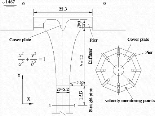
The basic parameters of the real vertical pipe inlet/outlet studied in this paper are presented in Figure 1. The system mainly consists of a straight pipe, diffuser, piers and cover plate along the stream-wise direction of pumping mode. The diameter of the straight pipe is D = 5.2 m. The diffuser with a length of 22 m adopts a 1/4 elliptical curve, for which the equation is x²/5.65²+y²/22²=1. There are 8 piers with a thickness of 1.2 m around the exit of the diffuser, which divide the inlet/outlet into 8 diversion orifices, and the height of diversion orifices is H = 3 m. The water level of the upper reservoir is 1467 m. The discharge rate for pumping mode and generating mode are 93.52 m³/s and 108.36 m³/s, respectively.

Figure 1. Geometry of the real vertical pipe inlet/outlet (dimensions in m).

3. Simulation method

3.1. Governing equations

It was assumed that the turbulence studied in this paper is isothermal and incompressible. The flow field for three-dimensional geometry is determined by solving the steady Reynolds-averaged continuity and momentum equations: (1) (2) where and are the velocity and the coordinate components, respectively; is the time; is the pressure; is the fluid density and is the kinetic viscosity; is the Reynolds stress; represents the velocity fluctuation in the i-direction.

To closure the Formula (1) and (2), a suitable turbulence model should be chosen. As one of the most popular RANS models, SST combines the advantages of k-ϵ and k-ω models and was first introduced by Menter (1994). For the SST model, near-wall resolution is particularly important because the near-wall modeling is based on the ω-formulation, which can be integrated through the viscous sublayer. However, cost and speed of the analysis are of crucial importance for shape parameter studies. For large-scale industrial flows the SST requirement y+ < 5 is excessive, especially when the Reynolds number is relatively high. In engineering applications the k-ϵ family models with wall functions, which allows the use of coarser grids, are preferred. Although the standard k-ϵ model is robust, efficient and very widely used, it is known that in flows where a significant stream curvature or strong pressure gradient exists, this model becomes inadequate. The realizable k-ϵ model, in contrast, is likely to provide superior performance for flows involving rotation and boundary layers with strong adverse pressure gradients, separation, and recirculation. The realizable k-ϵ model has been validated for a variety of flows, including jet, mixing layer, channel, boundary layer, rotating and separated flows. In this paper, therefore, the realizable k-ϵ model was selected for the numerical simulation. The modeled transport equations for the turbulence kinetic energy, , and its rate of dissipation, , in the realizable k-ϵ model (Shih, Liou, Shabbir, Yang, & Zhu, 1995) are (3) (4) where is the generation of turbulence kinetic energy due to the mean velocity gradients, , , ; is the kinetic viscosity; and are the turbulent Prandtl numbers for and , respectively. , . The model constants are  = 1.9,  = 1.0,  = 1.2, which can be found in the Fluent User’s Guide (Ansys Fluent, 2015).

The eddy viscosity is computed from (5) where , , , is the mean rate-of-rotation tensor viewed in a moving reference frame with the angular velocity . The model constants  = 4.04, , , , .

3.2. Grids and boundaries

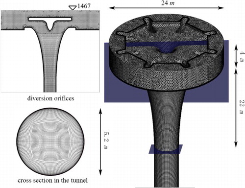
The computational domain covered a 20D long straight pipe to ensure a fully developed flow in the straight pipe. The reservoir outside boundary was located 20D from the center of the cover plate. As the shape of simulated domain is irregular, both structured and unstructured grids were used in different regions according to the boundary shape and the flow features. The minimum grids with a length of 0.1H were located at diversion orifices. The wall-normal mesh near the wall was refined to meet the non-equilibrium wall function (Kim & Choudhury, 1995), the minimum size of which was determined as 0.001D after several trials. After the calculation, y+ was checked of which the vast majority was between 30 and 300. The total grid number was approximately 8,956,000, which could achieve convergent and mesh-independent solutions. Figure 2 shows a schematic diagram of grids employed in the computational domain.

Figure 2. Schematic diagram of the vertical pipe inlet/outlet geometry with computational grids.

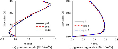
In order to evaluate the grid independence of the results, tests on velocity distribution were undertaken with the final grid used, as well as one coarser and one finer. And the two additional grid numbers were roughly 5,268,000 (Grid 1) and 13,532,000 (Grid 2) cells in total, respectively. Results for velocity distribution of the orifice at different refinement levels are given in Figure 3, which suggest that the medium grid solution is sufficient already for the engineering simulations.

Figure 3. Comparisons of velocity distribution at the diversion orifice with different resolution grids.

For pumping mode, the inlet of the straight pipe was defined as the inflow boundary, where a uniform mean velocity was assumed. The turbulence intensity I and hydraulic diameter D_h = D were employed at inflow boundary. As stated in the Ansys Fluent User’s Guide (2015), the turbulence intensity at the core of a fully-developed duct flow can be estimated from the following formula derived from an empirical correlation for pipe flows: (6) where is Reynolds number determined by hydraulic diameter which is equal to the diameter of the circular pipe. At the outflow boundary a constant reservoir level was imposed. While for generating mode, the flow is in the opposite direction. The rigid-lid hypothesis for the free surface was used because of the small fluctuations of the water level observed in the experiment. This hypothesis is widely used for the water surface treatment, and the free surface is treated as a horizontal rigid lid where symmetry conditions are applied for the velocity components (Booij, 2003; Kara, Kara, Stoesser, & Sturm, 2015; van Balen, Uijttewaal, & Blanckaert, 2009, 2010). Although more complex free surface treatment techniques may be more accurate to capture the motion of water surface, such simulations will be time-consuming and restricted by the available computer resources. All solid surfaces were set to be of the no-slip boundary condition where a non-equilibrium wall function was used. The wall equivalent roughness height can be computed from Manning’s n, the expression is (Marriott & Jayaratne, 2010), with dimensions in meters. Manning’s coefficient for concrete is taken as 0.014, so the surface roughness  = 2.2 × 10⁻³ m. The boundary conditions and turbulence settings applied to the model were also shown in Table 1.

Table 1. Boundary conditions and turbulence settings applied in the simulations.

Parameters	Notes	Values
Inlet (pumping mode)	The inlet of the straight pipe was defined as velocity inlet.	V = 4.406 m/s
Outlet (pumping mode)	Reservoir outside boundary was defined as pressure outlet.	Relative pressure: 0 Pa
Inlet (generating mode)	Reservoir outside boundary was defined as pressure inlet.	Relative pressure: 0 Pa
Outlet (generating mode)	The inlet of the straight pipe was defined as velocity outlet.	V = 5.105 m/s
Free surface	According the rigid-lid hypothesis, symmetry condition was applied.	——
Wall condition	The no-slip boundary condition was selected.	ks = 2.2 × 10^−3 m
Turbulence	Adopting the realizable k-ϵ model and the non-equilibrium wall function.	——
Grid number	——	8,956,000

The governing equations for the conservation of mass, momentum and transport equations were discretized using the finite volume method with the commercial CFD package Ansys Fluent 17.0. Considering the great grid number and small grid size near the orifice, the single-phase simulations were implemented in steady-state conditions. Regarding the interpolation schemes of pressure, standard difference scheme was used. The algorithm adopted to solve the coupling between the pressure and velocity fields in the Navier-Stokes equations was SIMPLE. A second-order upwind scheme was used for the discretization of the convective terms. A conventional procedure to evaluate convergence uses residuals. All results were assumed converged when the residuals became less than 0.001 for all equations. In order to obtain a converged result, the processing CPU time for each condition was approximately 12 hours, which was managed by two personal computers equipped by Intel core i7 processors at 3.2 GHz and 16 GB of ram.

4. Validation of the computational model

Validation is the primary means to assess the accuracy and reliability of the computational model by comparison with experimental data (Oberkampf & Trucano, 2002), which is why an additional hydraulic experimental model test was carried out. The head losses in the system and velocity distribution at diversion orifices were measured, and compared with computational values.

The head losses of the vertical pipe inlet/outlet are mainly local head losses, and the calculation sections are cross section 0-0 that is reservoir level and cross section 1-1 located at a distance of 1.5D from the starting section of the diffuser, as shown in Figure 1. The measured local head loss is usually given as ratio of the head loss through the device to the velocity head V²/(2 g) of the associated piping system (White, 2011), which is dimensionless and commonly used as an important indicator to evaluate the performance of different hydropower stations. Based on the Bernoulli equation the head losses and coefficients of the head losses can be computed as follows: (7) (8) (9)

Where are the head losses, and for pumping mode and for generating mode; is coefficient of the head losses; and are piezometric head for reservoir level and section 1-1 respectively; is the average axial velocity of the straight pipe; is gravitational acceleration; is the kinetic energy correction factor and taken as 1.0 in this paper.

4.1. Physical model overview

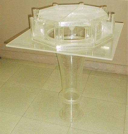
The experiments were conducted in the State Key Laboratory of Hydraulic Engineering Simulation and Safety, Tianjin University. Because the flow phenomena of the vertical pipe inlet/outlet are determined primarily by the gravitation, the Froude number similitude was used to describe the similitude relationships between the model and the real plant variables. A 1/33.77 scale was adopted for the hydraulic model test. To match the resistance similarity, the roughness scale was taken as 1/1.80. The concrete roughness is 0.014, so the model roughness value was 0.0078 for the scales of 1/1.80. To meet the needs of the roughness, the model was made of plexiglass, as illustrated in Figure 4.

Figure 4. A view of the experimental model of the inlet/outlet made of plexiglass.

An illustration of the experimental system is shown in Figure 5. A high constant-head tank was used to supply steady flow for the experimental model that was mounted at the center of another regular tank acting as the reservoir. The reservoir tank was supported by a platform 3.5 m above the floor.

Figure 5. Schematic diagram of the experimental setup.

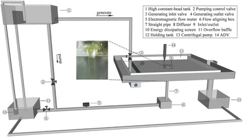
In the pumping mode, the generating control valves were close, while the pumping control valve was open. The flow from the constant-head tank passed through the vertical pipe outlet and then entered the reservoir tank. However, the realization requirements of our installation only allowed placing a 15D long vertical straight pipe, which was slightly shorter than the numerical simulations. To prevent disturbances due to the curvature of the joint between the horizontal and vertical pipe, a square box that can align the flow was used, instead of a bend pipe. The water level in the reservoir was controlled by overflow baffles around the tank, and finally the fluid fell into a lower holding tank, from which it was pumped back to the constant-head tank using a centrifugal pump.

In the generating mode, the pumping control valve was closed, while the generating valves were open. Water was conveyed to the reservoir tank through a vertical conduit connected to a horizontal diffuser pipe with lateral holes, which can distribute the water over the tank width. At the entrance there were energy-dissipating screens that can reduce inflow turbulence and make the flow as uniform as possible. The water level in the reservoir was controlled by the baffles, just like that in the pumping mode.

The experimental discharge for the pumping mode was 0.0141 m³/s, corresponding to a Reynolds number Re = 116,772 in the tunnel; while in the generating mode, the discharge was 0.0164 m³/s and the Reynolds number was 135,298. The flow rate to the model was adjusted by the control valve and was measured by an electromagnetic flow meter with an accuracy of 0.5% for the measured ranges. A Vectrino ADV instrument, developed by Nortek AS, was used to instantaneously measure stream-wise velocity of diversion orifices at various depths. Based on the Doppler shift principle, the ADV instrument can measure velocities with ± 1% accuracy in the measurement range of 1 mm/s. Each measurement point with a sampling volume of 7 mm worked at a sampling frequency of 50 Hz for 60 s of sampling time. Piezometric head of each section was read directly from Piezometric tube with an accuracy of 1 mm.

4.2. Comparison between computation and model test

Figure 6 shows comparisons of the numerical results against the experimental data for head losses coefficients of the diversion orifice. In order to better understand the results, the linear fit line equation with is plotted. Figures 7 and 8 demonstrate a correlation analysis of the head loss and the velocity head V²/(2 g) in the experiments and simulations. Based on these two figures and considering R², it can be said that the experimental and numerical results both show a stable head losses coefficient curve in different flow rate, which means the head losses of the vertical pipe inlet/outlet are mainly local head losses. However, some discrepancies between the measured and numerical data are observed. It is found that the set of experimental data is more volatile, which probably happens due to random and bias errors in the device installation and data measurement. Comparing the ratio of the linear fit line in Figures 7 and 8, although the numerical model slightly underestimates the head losses coefficients, it is still acceptable to predict the results of this engineering problem.

Figure 6. Head losses coefficients of simulations and experiments.

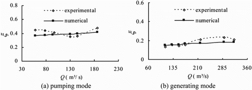
Figure 7. Correlation analysis of the head losses of experiments.

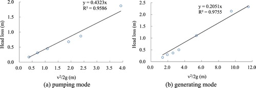
Figure 8. Correlation analysis of the head losses of simulations.

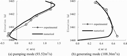
Figure 9 shows comparisons of the numerical results against the experimental data for velocity distribution of the diversion orifice. From the figure, the experimental and numerical results demonstrate the same velocity pattern of flow in the pumping mode and generating mode, respectively. The mainstream with higher velocity of the pumping mode is located near the upper part of the orifices, while near the lower in the generating mode. The velocity distribution along the height of the orifices in generating mode is more uniform than that in pumping mode. This phenomenon indicates that negative velocity region caused by the diffusion and turning flow in the pumping mode deserves more attention. In Figure 9(a), the numerical results overestimate the negative region a bit, which is acceptable because the number of measuring points in the experiment is limited to accurately capture the reverse flow zone. However, it should be noted that the boundary layer is not well resolved under generating mode in Figure 9(b), which may be caused by changes in y+ values between totally different operation modes. Although the enhanced wall treatment, which does not depend on y+ changes, is more suitable in the complex bidirectional problem, it will generate too many grids to apply for such large scale simulations. In view of the engineering situation, it is more important to concern the reverse flow zone under pumping mode that possibly induces vibration failure of trash racks. Therefore, it can be observed from the comparisons of the numerical and experimental results that the numerical head losses coefficients and velocity distribution basically agrees well with that of measurements, which indicates that the computational model used in this paper is reasonable and feasible to predict such complex three-dimensional flow in the vertical pipe inlet/outlet.

Figure 9. Velocity distribution of simulation and experiment at diversion orifice.

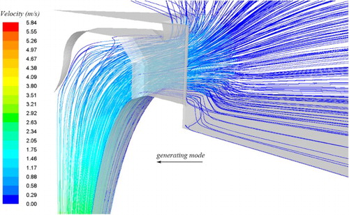
Figures 10 and 11 show 3D streamlines in the vertical inlet/outlet under pumping mode and generating mode, respectively. As can be seen, under pumping mode, the roll-up of the 3D streamlines near the outlet of the orifice shows an attached vortex that is generated due to flow separation at the end of the diffuser and rapid change of flow direction. The vortex extends and causes reverse flow zone at the bottom of diversion orifice, which is circled in red in Figure 10. Whereas the 3D streamlines smoothly flow through the inlet of the orifice under generating mode, which can be considered as contraction flow and shows a better flow pattern.

Figure 10. 3D velocity streamlines in the vertical outlet under pumping mode.

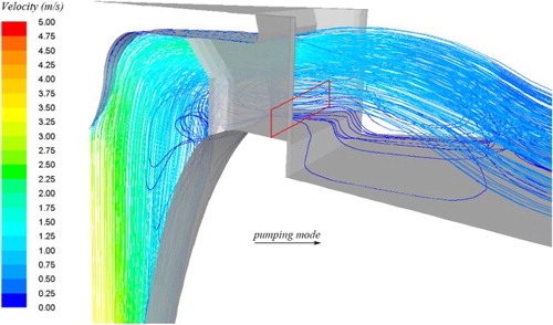
Figure 11. 3D velocity streamlines in the vertical inlet under generating mode.

5. Computational results and discussion

5.1. Effect of diversion orifices height

For the pumped storage plant, the pipe diameter is commonly predetermined by many factors, such as economy benefit, local demand and so on. In view of this, the diameter D can be seen as a representative parameter whose value is fixed in the paper, and the various heights are normalized by it to analyse typically. In addition, in order to analyse the effect of diversion orifices height, the divergence angle is a/b = 0.257 for each configuration.

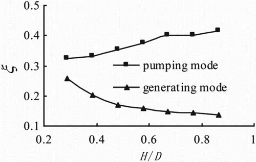
Figure 12 shows the total coefficient of head losses of the vertical pipe inlet/outlet for various heights of diversion orifices. It can be seen that the head losses substantially depend on the height of the diversion orifices. The head losses of pumping mode are bigger than that of generating mode due to the diffusion flow under pumping mode while contraction flow under generating mode. With increase of the relative height of the diversion orifices, the head losses coefficient of pumping mode gradually increases, but the head losses coefficient of generating mode gradually reduces, especially when H/D = 0.288–0.481, the head losses coefficient of generating mode gets a rapid reduction.

Figure 12. Head losses coefficients in different diversion orifices heights.

Figure 13 shows the profiles of the streamwise velocity over the height of the diversion orifices in different diversion orifices heights. In these figures, the velocities at different monitoring points are normalized by the mean velocity at the inlet of the straight pipe , and the diversion orifices heights are normalized by the straight pipe diameter D.

Figure 13. Velocity distribution at diversion orifice in different diversion orifices heights.

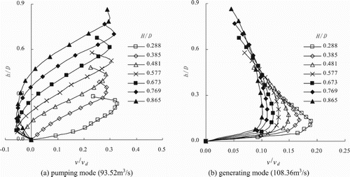
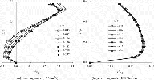
It can be observed that under pumping mode, the shapes of the velocity curves are similar in different diversion orifices heights which present a large upper part and small lower part, and the peak velocity is all located on the upper part of the orifices, approximately 91 percent of orifice height away from the bottom. The reverse flow (the fluid flowing back into the orifices) occurs at the bottom of the diversion orifices, with the exception of H/D = 0.288 and H/D = 0.385. Moreover, the height of the reverse flow zone gradually increases with increasing height of the diversion orifices. When H/D = 0.865, the height of the reverse flow zone even reaches half the real height of the orifices, which directly leads to an additional head loss. With increase of the relative height of the diversion orifices, mean velocity of the orifices should reduce. However, because of increasing height of the reverse flow zone, the maximum velocity of the orifices does not show an obvious reduction.

In the generating mode, with increase of the relative height of the diversion orifices, the maximum velocity of the orifice from 0.190 to 0.101 reduces evidently, and the velocity distribution along the height of the orifices tends to be more uniform, as a result, to a reduction in head loss.

It can be seen from the above analysis that inflow and outflow are contradictory, for instance, the higher in orifices, the better for inflow; however, it is not favorable for outflow. Taking into account the head losses, the maximum velocity of the diversion orifices and the height of the reverse flow zone in the pumping mode and generating mode, the diversion orifices heights in the range H/D = 0.481–0.577 are suitable.

5.2. Effect of divergence angle

Because the diffuser adopts a 1/4 elliptical curve that is controlled by the equation x²/a²+y²/b²=1, the divergence angles can be changed by adjusting values of a and b. However, the elevation at the bottom of the reservoir is usually not feasible to change. It is more appropriate to achieve various divergence angles through adjusting values of a, while b is a constant in the study. Besides, the analysis of the divergence angle is performed for the diversion orifices height H/D = 0.577.

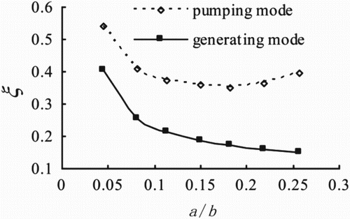
Figure 14 shows the total coefficient of head losses of the vertical pipe inlet/outlet for various divergence angles. In the pumping mode, the head losses coefficient of pumping mode decreases first and then increases with increase of the divergence angle. Minimum head loss is noted when the divergence angle a/b = 0.182. While with increase of the divergence angle, the head losses coefficient of the generating mode gradually reduces, especially when a/b = 0.045–0.082, the head losses coefficient gets a rapid reduction.

Figure 14. Head losses coefficients in different divergence angles.

Figure 15 shows the profiles of the streamwise velocity over the height of the diversion orifices in different divergence angles.

Figure 15. Velocity distribution at diversion orifice in different divergence angles.

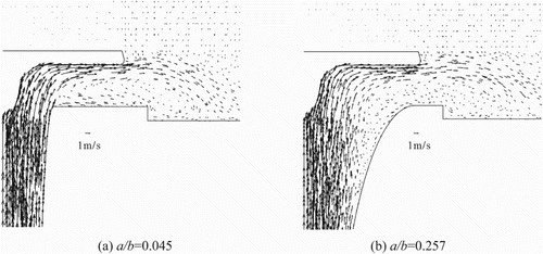
In the pumping mode, with increase of the divergence angle, the height of the reverse flow zone at the bottom of diversion orifice gradually reduces and the maximum velocity of the orifice gradually decreases. The head losses coefficient of pumping mode mainly depends on the flow separation in the diffuser and at the bottom of diversion orifice. It can be seen from the flow pattern of the vertical pipe inlet/outlet, as shown in Figure 16, that the flow separation mainly occurs at the bottom of the diversion orifice, and there is basically no separating phenomenon in the diffuser when a/b = 0.045, therefore the head losses of the system mainly occur at the diversion orifice after the diffuser. While when a/b = 0.257, the flow separation occurs both at the bottom of diversion orifice and the diffuser, and the head losses of the system contain these two parts.

Figure 16. The flow pattern in the vertical pipe inlet/outlet.

In the generating mode, the velocity distributions of the diversion orifices in different divergence angles are almost identical, which indicates that divergence angle has little influence on velocity distribution.

Taking into account the head losses, the maximum velocity of the diversion orifices and the height of the reverse flow zone in the pumping and generating mode, the divergence angles of the diffuser in the range a/b = 0.182–0.218 are suitable.

6. Conclusions

In this paper, the characteristics of turbulent flow through a vertical pipe inlet/outlet with a horizontal anti-vortex plate were studied. The realizable k-ϵ model was employed to obtain the depth velocity distribution and head losses in the diversion orifices using CFD software. To verify the turbulence model, the experiment with original shape was applied. The comparison of the numerical and experimental results showed that the numerical head losses coefficients and velocity distribution basically agrees well with that of measurements. Based on the comparison with the experiment, the flow characteristics of the vertical pipe inlet/outlet was further investigated under different geometries and working conditions. It was found that variations including changes in diversion orifices height as well as in divergence angle have a significant impact on hydraulic characteristics of the inlet/outlet. Besides, the hydraulic characteristics of the pumping mode and that of the generating mode are contradictory, and the optimal conditions cannot be achieved simultaneously. Therefore, we then turned our attention to finding sets of the shape parameters which are acceptable for the flow conditions both in the pumping and generating mode. With consideration of the head losses, the maximum velocity of the diversion orifices and the height of the reverse flow zone, the relative height of the diversion orifices in the range H/D = 0.481–0.577 and the divergence angle of the diffuser in the range a/b = 0.182–0.218 are preferable. The results provide important evidence for guiding the design of the vertical pipe inlet and outlet of pumped storage plants. However, some limitations are worth noting. Although we tried to adopt as many sets of shape parameters as we can, it was difficult and time consuming to determine the best design manually by parametric studies. As a future study, it would be interesting to apply multi-objective optimization algorithms coupled with CFD software to solve optimization problems of the vertical pipe inlet and outlet.

Disclosure statement

No potential conflict of interest was reported by the authors.

ORCID

Bowen Sun http://orcid.org/0000-0002-8526-9070

Additional information

Funding

The present study was supported by the Science Fund for Creative Research Group of the National Natural Science Foundation of China [grant number 51621092], [grant number 51279125].

References

- Aloui, F., Berrich, E., & Pierrat, D. (2011). Experimental and numerical investigations of a turbulent flow behavior in isolated and nonisolated conical diffusers. Journal of Fluids Engineering, 133, 011201. doi: 10.1115/1.4003236
- Ansys Fluent. (2015). User’s and theory guide. Canonsburg, PA: ANSYS, Inc.
- Booij, R. (2003). Measurements and large eddy simulations of the flows in some curved flumes. Journal of Turbulence, 4. doi: 10.1088/1468-5248/4/1/008
- Chau, K. W., & Jiang, Y. W. (2001). 3D numerical model for pearl river estuary. Journal of Hydraulic Engineering, 127(1), 72–82. doi: 10.1061/(ASCE)0733-9429(2001)127:1(72)
- Chau, K. W., & Jiang, Y. W. (2004). A threedimensional pollutant transport model in orthogonal curvilinear and sigma coordinate system for pearl river estuary. International Journal of Environment and Pollution, 21(2), 188–198. doi: 10.1504/IJEP.2004.004185
- Chen, Y.-l., Wu, C., Ye, M., & Ju, X.-m. (2007). Hydraulic characteristics of vertical vortex at hydraulic intakes. Journal of Hydrodynamics, Ser. B, 19(2), 143–149. doi: 10.1016/S1001-6058(07)60040-7
- Chen, Z., Ettema, R., & Lai, Y. (2004). Ice-tank and numerical study of frazil ingestion by submerged intakes. Journal of Hydraulic Engineering, 130(2), 101–111. doi: 10.1061/(ASCE)0733-9429(2004)130:2(101)
- Echávez, G., & McCann, E. (2002). An experimental study on the free surface vertical vortex. Experiments in Fluids, 33(3), 414–421. doi: 10.1007/s00348-002-0463-2
- El-Behery, S. M., & Hamed, M. H. (2011). A comparative study of turbulence models performance for separating flow in a planar asymmetric diffuser. Computers & Fluids, 44, 248–257. doi: 10.1016/j.compfluid.2011.01.009
- Gowda, B. H. L., Joshy, P. J., & Swarnamani, S. (1996). Device to suppress vortexing during draining from cylindrical tanks. Journal of Spacecraft and Rockets, 33(4), 598–600. doi: 10.2514/3.26806
- Gowda, B. H. L., & Udhayakumar, H. (2005). Vane-type suppressor to prevent vortexing during draining from cylindrical tanks. Journal of Spacecraft and Rockets, 42(2), 381–383. doi: 10.2514/1.8624
- Greifzu, F., Kratzsch, C., Forgber, T., Lindner, F., & Schwarze, R. (2016). Assessment of particle-tracking models for dispersed particle-laden flows implemented in OpenFOAM and ANSYS FLUENT. Engineering Applications of Computational Fluid Mechanics, 10(1), 30–43. doi: 10.1080/19942060.2015.1104266
- Kara, S., Kara, M. C., Stoesser, T., & Sturm, T. W. (2015). Free-Surface versus rigid-Lid LES computations for bridge-abutment flow. Journal of Hydraulic Engineering, 141(9), 04015019. doi: 10.1061/(ASCE)HY.1943-7900.0001028
- Kim, S. E., & Choudhury, D. (1995). A near-wall treatment using wall functions sensitized to pressure gradient. Separated and Complex Flows, 217, 273–280.
- Kocabas, F., & Unal, S. (2010). Compared techniques for the critical submergence of an intake in water flow. Advances in Engineering Software, 41(5), 802–809. doi: 10.1016/j.advengsoft.2009.12.021
- Kocabaş, F., Ünal, S., & Ünal, B. (2008). A neural network approach for prediction of critical submergence of an intake in still water and open channel flow for permeable and impermeable bottom. Computers & Fluids, 37(8), 1040–1046. doi: 10.1016/j.compfluid.2007.11.002
- Lee, J., Jang, S. J., & Sung, H. J. (2012). Direct numerical simulations of turbulent flow in a conical diffuser. Journal of Turbulence, 13, 1–29. doi: 10.1080/14685248.2011.633522
- Li, H.-f., Chen, H.-x., Ma, Z., & Zhou, Y. (2009). Formation and influencing factors of free surface vortex in a barrel with a central orifice at bottom. Journal of Hydrodynamics, Ser. B, 21(2), 238–244. doi: 10.1016/S1001-6058(08)60141-9
- Mahyari, M. N., Karimi, H., Naseh, H., & Mirshams, M. (2010). Numerical and experimental investigation of vortex breaker effectiveness on the improvement in launch vehicle ballistic parameters. Journal of Mechanical Science and Technology, 24(10), 1997–2006. doi: 10.1007/s12206-010-0618-7
- Marriott, M. J., & Jayaratne, R. (2010). Hydraulic roughness – links between Manning’s coefficient, Nikuradse’s equivalent sand roughness and bed grain size. Proceedings of Advances in Computing and Technology, (AC&T) The School of Computing and Technology 5th Annual Conference, University of East London, pp. 27–32.
- Menter, F. R. (1994). Two-equation eddy-viscosity turbulence models for engineering applications. AIAA Journal, 32(8), 1598–1605. doi: 10.2514/3.12149
- Mizuki, S., Gowda, B. H. L., & Uchibaba, T. (2003). Visualization studies using PIV in a cylindrical tank with and without vortex suppressor. Journal of Visualization, 6(4), 337–342. doi: 10.1007/BF03181740
- Nabavi, M. (2010). Three-dimensional asymmetric flow through a planar diffuser: Effects of divergence angle, Reynolds number and aspect ratio. International Communications in Heat and Mass Transfer, 37, 17–20. doi: 10.1016/j.icheatmasstransfer.2009.08.006
- Naderi, V., Farsadizadeh, D., Hosseinzadeh Dalir, A., & Arvanaghi, H. (2014). Effect of using vertical plates on vertical intake on discharge coefficient. Arabian Journal for Science and Engineering, 39(12), 8627–8633. doi: 10.1007/s13369-014-1468-x
- Oberkampf, W. L., & Trucano, T. G. (2002). Verification and validation in computational fluid dynamics. Progress in Aerospace Sciences, 38(3), 209–272. doi: 10.1016/S0376-0421(02)00005-2
- Özkan, F., Wenka, A., Hansjosten, E., Pfeifer, P., & Kraushaar-Czarnetzki, B. (2016). Numerical investigation of interfacial mass transfer in two phase flows using the VOF method. Engineering Applications of Computational Fluid Mechanics, 10(1), 100–110. doi: 10.1080/19942060.2015.1061555
- Pérez-Díaz, J. I., Chazarra, M., García-González, J., Cavazzini, G., & Stoppato, A. (2015). Trends and challenges in the operation of pumped-storage hydropower plants. Renewable and Sustainable Energy Reviews, 44, 767–784. doi: 10.1016/j.rser.2015.01.029
- Sarkardeh, H., Reza Zarrati, A., Jabbari, E., & Marosi, M. (2014). Numerical simulation and analysis of flow in a reservoir in the presence of vortex. Engineering Applications of Computational Fluid Mechanics, 8(4), 598–608. doi: 10.1080/19942060.2014.11083310
- Selvam, K., Peixinho, J., & Willis, A. P. (2015). Localised turbulence in a circular pipe flow with gradual expansion. Journal of Fluid Mechanics, 771, 123. doi: 10.1017/jfm.2015.207
- Shih, T.-H., Liou, W. W., Shabbir, A., Yang, Z., & Zhu, J. (1995). A new k-ϵ eddy viscosity model for high reynolds number turbulent flows. Computers & Fluids, 24(3), 227–238. doi: 10.1016/0045-7930(94)00032-T
- Sohn, C. H., Ju, M. G., & Gowda, B. H. L. (2009). Draining from cylindrical tanks with vane-type suppressors - A PIV study. Journal of Visualization, 12(4), 347–360. doi: 10.1007/BF03181878
- Sparrow, E. M., Abraham, J. P., & Minkowycz, W. J. (2009). Flow separation in a diverging conical duct: Effect of Reynolds number and divergence angle. International Journal of Heat and Mass Transfer, 52(13), 3079–3083. doi: 10.1016/j.ijheatmasstransfer.2009.02.010
- van Balen, W., Uijttewaal, W. S. J., & Blanckaert, K. (2009). Large-eddy simulation of a mildly curved open-channel flow. Journal of Fluid Mechanics, 630, 413. doi: 10.1017/S0022112009007277
- van Balen, W., Uijttewaal, W. S. J., & Blanckaert, K. (2010). Large-eddy simulation of a curved open-channel flow over topography. Physics of Fluids, 22(7), 075108. doi: 10.1063/1.3459152
- White, F. M. (2011). Fluid mechanics (7th ed.). New York: McGraw-Hill.
- Wu, C. L., & Chau, K. W. (2006). Mathematical model of water quality rehabilitation with rainwater utilization — a case study at Haigang. International Journal of Environment and Pollution, 28(3–4), 534–545. doi:https://doi.org/10.1504/IJEP.2006.011227
- Xie, J., & Jin, Y.-C. (2016). Parameter determination for the cross rheology equation and its application to modeling non-Newtonian flows using the WC-MPS method. Engineering Applications of Computational Fluid Mechanics, 10(1), 111–129. doi: 10.1080/19942060.2015.1104267
- Yang, J., Liu, T., Bottacin-Busolin, A., & Lin, C. (2014). Effects of intake-entrance profiles on free-surface vortices. Journal of Hydraulic Research, 52(4), 523–531. doi: 10.1080/00221686.2014.905504
- Ye, F., & Gao, X.-p. (2011). Numerical simulations of the hydraulic characteristics of side inlet/outlets. Journal of Hydrodynamics, Ser. B, 23(1), 48–54. doi: 10.1016/S1001-6058(10)60087-X