Design criteria for a type of asymmetric orifice in a surge tank using CFD

ABSTRACT

An asymmetric orifice can be added to a surge tank of a hydro power plant to dampen the mass oscillation. This allows a reduction of the required volume and a more stable behavior of the overall hydraulic system. In this paper, the advantage of a typical asymmetric orifice is shown in comparison with a sharp-edged geometry with two different pipe diameters. The software ANSYS-CFX is used to investigate the influence of the individual geometry parameters (radius, length, angle at the forefront) on the local head loss coefficients and the ratio of the two flow directions. Furthermore, a coefficient is analyzed based on an equation from the literature for the sharp-edged structure, which can be used comparably for the asymmetric orifice. This allows us to reach preliminary assumptions of the losses at an early state of the design process. The following adaptation can be supported by the presented guidance for the optimization process, so that a suitable geometry for the specific boundary conditions can be found.

KEYWORDS:

• Control structures
• flows in pipes and nozzles
• hydraulics of renewable energy systems
• hydraulic structure design and management
• RANS model

1. Introduction

An orifice allows the introduction of an additional head loss at a specific location of a hydraulic system, which is useful for multiple applications. For example, standardized shapes allow the measurement of the discharge Q through a pipe while monitoring the pressure differences on both sides of the device (ASME, 2004; EN ISO, 2003). In connection with a spillway, such a structure can be added to dissipate a large amount of energy (Jianhua et al., 2010; Zhang & Chai, 2001). This paper focuses on applications that work as a throttle in a surge tank of a hydro power plant (HPP).

The surge tank is a vital part of a hydraulic system and allows a reduction in the impact of a change in the operation mode. It is often designed solely for one specific project, depending on the particular hydraulic and geological boundary conditions (BCs). Stability criteria define the minimum area of the shaft (Thoma, 1910; Ye et al., 1992) and the storage capacity can be enhanced with additional chambers. Large mass oscillations between the surge tank and the upper reservoir can be further damped with the addition of a throttle (Adam et al., 2018a; Li & Brekke, 1989; Vereide et al., 2017). Such a structure can be added in the connection between the surge tank and head race tunnel or at a change of the cross section (Adam et al., 2016a; Richter et al., 2015). The use of an asymmetric geometry further allows us to limit the loss in the upward flow direction (into the surge tank) and to add a bigger damping effect on the downward flow direction. This leads to a reduction of the required volumes in the surge tank without introducing unwanted limits in the operation of the HPP. Extreme combination of losses can be reached with a vortex chamber diode, which has the disadvantage that the full throttling loss is available after an initialization time (Haakh, 2003). Hence, an asymmetric orifice is often preferred, which provides a stable behavior as well as a suitable ratio of the losses depending on the flow direction.

Tabular values can provide a preliminary assumption of the local head loss coefficient of the orifice at an early design phase. Further refinements are conducted based on scaled model tests and also computational fluid dynamics (CFD) methods. Both are capable of quantifying the losses based on the specific design (Adam, 2017; Adam et al., 2016a,b; Gabl, 2012; Gabl et al., 2014a,b, 2017; Huber, 2010; Vereide et al., 2015a,b). Those coefficients are input values for the global optimization of the surge tank beside geometry and hydraulic BCs of the HPP.

The paper presents a variation of the basic geometry parameters of a typical asymmetric orifice with the software ANSYS-CFX. The results are used to adapt the equation for sharp changes with different pipe diameters given by Idelchik (1960). This allows us to quantify the loss of such a specific structure compared to other shapes covered in the literature. Furthermore, a guide for the optimization process is developed, which can help to find a suitable asymmetric orifice for the specific BCs of a future project.

2. Materials and methods

2.1. Basic equations

The local head loss can be calculated as (1) which is based on the Bernoulli equation comparing two different cross sections. Those are numbered in the flow direction and for each of them the pressure p, velocity v (average value of the complete cross section), and the kinetic energy correction coefficient α (real kinetic energy divided by theoretical value ) is evaluated. The density ρ of the fluid (water) as well as the gravity acceleration g are simplified as constants. The local head loss coefficient ζ is defined as a factor on the kinetic energy head using a reference velocity . Thereby, it is assumed that the coefficient is only dependent on the geometry for turbulent flow conditions and that the transient behavior is comparably small (Adam, 2017; Gabl et al., 2014a; Kobus, 1987,1980).

In general, the cross section downstream of the loss is used to calculate the . To allow a better comparison of the geometry analysis, the fixed cross section and velocity is always used as a reference in this paper. If the two different sections have the same geodetic height, and are equal and also the gravity acceleration g can be reduced: (2)

In the case of an asymmetric orifice the local head loss depends on the flow direction ( in downward and in upward flow direction) and therefore the parameter λ is used to quantify this effect: (3)

The numerical results are compared with an approach from the literature. The equation given by Idelchik (1960) allows us to evaluate the local loss coefficient for an orifice at the passage of a stream from a conduit of one size to another, which is similar to the reference geometry shown in Figure 1(a). In (4) the original equation is adapted to the nomenclature based on the reference geometry (Section 2.2) and exemplarily presented for the upward direction. With the factor the reference velocity is changed from to . The approach joins the sudden changes (contraction and expansion) with an interaction part and the variable Ψ is introduced. This variable is further evaluated to investigate the dominant cause of the loss. In the case of small Ψ-values, the sudden expansion is the dominant cause of the loss.

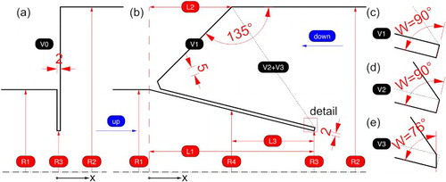
Figure 1. Profile curve of the reference geometry with (a) only sudden changes and (b) the typical shape of an asymmetric orifice. (c)–(e) Detailed view of the geometry versions , , and . All lengths in millimeters.

2.2. Reference geometry

The investigated reference geometry is chosen according to the new asymmetric orifice in the surge chamber of the HPP Kaunertal (Bonapace, 2012; Gabl, 2012; Gabl et al., 2014b; Richter et al., 2015), which is owned by the TIWAG-Tiroler Wasserkraft AG and was put into operation at the end of May 2016. For the investigation, only the basic shape of the asymmetric orifice is used and further simplified, so that it can be generally used. All investigated shapes are rotation-symmetric around the x-axis, which is the main flow direction.

The key parameter for the standardization is the radius of the pipe, which represents the inflow boundary for the upward flow condition. For the presented investigations a fixed value of 0.05 m for is chosen (typical value for a scale model test). The thickness of the orifice is fixed at 2 mm and the outer part of the orifice is chamfered with a value of 5 mm to reach a better numerical grid. The other parameters are defined based on Figure 1 and Table 1. The length is only used for the exact location of the radius and not tested separately.

Table 1. Reference geometry.

parameter	initial value
	0.05 m
W

Four different basic configurations are tested. The geometry only includes sudden changes in the cross section and is presented in Figure 1(a). This shape is comparable with that given by Idelchik (1960). The basic definition of the further investigated asymmetric orifice is called . Two slightly different variations are added. For the version the outer part is filled as presented in Figure 1(d). The version is defined similarly to , but the angle W is changed, so that the thickness of the orifice is perpendicular to the axis. Here and are used to investigate the influence of the outer geometry definition especially on the downward local head loss coefficient.

2.3. Numerics

2.3.1. General

For this study the 3D numerical software ANSYS-CFX (Version 17.2) was chosen. The investigation and optimization of turbines and turbo machinery blades (Teran et al., 2016; Zhang et al., 2012; Zhao et al., 2016) are typical application areas for this software. Nevertheless, examples of successful application can also be found in a wide range of cases: from wind forces on photovoltaic panels (Edgar et al., 2015) to anti-icing systems for wings (Hannat et al., 2014) or hydro power intakes (Bermúdez et al., 2017; Gabl et al., 2018). This commercial code is well validated for free surface (Andersson et al., 2013; De Cesare et al., 2001) and pressurized flow conditions (Adam et al., 2016b; Adane et al., 2008; Gabl et al., 2014b, 2018; Seibl, 2016; Seibl et. al, 2017).

All simulations of the presented study are conducted with double precision to ensure that no round-off error occurs. The fluid (water) is considered at constant temperature and density, therefore no buoyancy model has to be activated (Equation (2(2) )). The standard shear stress transport (SST) turbulence model (Menter, 1994; Menter et al., 2003) is chosen to solve the closure problem. It combines a k–ω-approach with a k–ε-model for the outer region including a blending function. This model is widely used in ANSYS products but also in connection with other CFD-codes (Yi et al., 2017). Different validations experiments of comparable structures show a very good agreement for comparable investigations with the SST-turbulence model (Adam, 2017; Alligne et al., 2014; Gabl et al., 2014b; Seibl, 2016). The investigated geometry is fully parametrized and the mesh is generated with the tool in ANSYS-Workbench. Two simulations are conducted to cover both flow directions for each variation of the investigated geometry parameter.

2.3.2. Boundaries

The basic geometry, as presented in Figure 1, is extended with a pipe of up to in length in both directions. Hence, the influence of the chosen BCs can be minimized. To simplify the simulation, only a segment of 24 is cut out of the rotation symmetrical geometry (Figure 2). A symmetry BC is defined at both cutting sides.

Figure 2. Exemplary results of the geometry (upper row) and (lower row) for upward (left column) and downward (right column) flow direction.

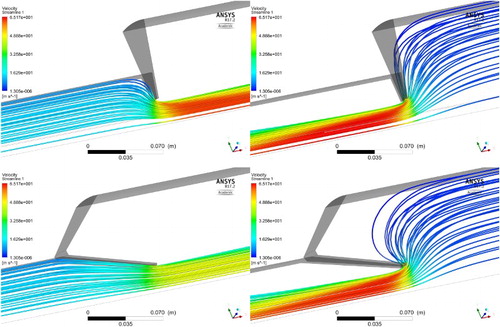
A fixed Reynolds number R of (–) at the pipe with the radius is chosen, which ensures that the local head loss coefficient is independent of the flow condition and can also be used for nature scale structures. This leads to a discharge Q equal to 0.079 m³ s⁻¹ (kinematic viscosity m² s⁻¹). Consequently, the homogeneous inlet velocity is 10 m s⁻¹ for the upward flow direction and 2.5 m s⁻¹ (default value ) for the reversed direction depending on the investigated radius . A pressure of 10 bar is predefined at the outlet BC, so that no negative pressure can occur in the model. Based on such a high R, it can be assumed that the local head loss coefficient is independent of the discharge and pressure (Büker et al., 2013; Lakshmana Rao et al., 1977). Exemplary results for the two basic geometry types are presented in Figure 2.

2.3.3. Post-processing

As a first step of the post-processing, a proper choice of the two reference cross sections has to be made. Based on those the results of the numerical simulations are evaluated to calculate the local head loss coefficient ζ given by Equation (2(2) ). Constant values are used for the upward and downward distance. Each one is related to the origin of the local coordinate system, which is located at the beginning of the orifice in the upward flow direction (Figure 1). This allows a good comparability for all variations of the orifice. Cross section 1, which is the first in the flow direction, is fixed at a distance of 6 upstream of the orifice. Decisive for this is the total length in the downward flow direction.

The flow is concentrated into a jet at the orifice both for upward and downward flows, which leads to a disturbed flow profile. Hence, the second reference cross section downstream of the orifice should be outside the recirculation zones. Typically for a thin orifice without a change of the diameter, a distance of 3– is considered (Jianhua et al., 2010; Roul & Dash, 2012). Idelchik (1960) recommends a value of 8– in case of a sudden expansions where a jet is observed.

Figure 3 shows the calculated ζ-value in relation to the distance x (Figure 1) of the second cross section (downstream of the orifice) to the origin. Those values are computed with the calculated energy correction factor α (α-index) and once with the assumption that the α-value is equal to 1.0 (-). Such a simplification is often used for an experimental set-up, in which no measured velocity profiles are available. Big changes of the calculated local head loss coefficient ζ can be found near the orifice (x smaller than approximately ), which are cause by the inhomogeneity of the flow conditions in this zone. After a certain distance, the value only increases caused by friction. Ideally this point is used to specify the local head loss coefficient ζ of the orifice.

Figure 3. Evaluation of the ζ-value depending on the distance x between the origin and the second cross section: (a) overview and (b) detail.

The pressure p, average velocity v, and energy correction factor α are separately analyzed in Figure 4. It can be observed that corresponding to the local increase of the velocity, the pressure drops. Those changes were caused by the inhomogeneity of the flow near the orifice and lead to an unrealistic local head loss coefficient (Figure 3). The α-value is a good indicator for nearly uniform flow conditions and, hence, it is chosen as a key parameter for the decision where the downstream cross section is situated. For all simulations a distance of upstream and (identical to the higher level suggested by Idelchik (1960)) downstream of the orifice is chosen. This section is marked in Figures 3 and 4 as a dashed line and shows nearly uniform velocity distributions for the majority of the simulations. An increased uncertainty should be considered in case of extreme geometry values.

Figure 4. Value of the pressure, velocity, and α-value (standardized by the value of ) depending on the distance x between the origin and the second cross section: (a) overview and (b) detail.

Each solution is checked manually for errors (streamlines, vectors, cross section). Furthermore, the variable Ψ is evaluated individually based on Equation (4(4) ) as well as the λ-ratio (Equation (3(3) )) for each geometry variation.

2.3.4. Verification

All numerical assumptions are checked in the preliminary verification process based on the reference geometry (Section 2.2) with the initial values for the parameter (Table 1). As an example, the results of the following tests are shown:

• definition of the BC (Table 2);

• size of the cut out segment (Table 3);

• thickness of the first layer mesh near the wall (Table 4);

• mesh resolution (Table 5).

Table 2. Basic investigations of boundary conditions (BC): current simulation and deviation in relation to the original value.

current	17.49	17.23	29.38	29.04
repetition	0.00%	0.00%	0.00%	0.00%
exchange BC	−0.06%	−0.03%	−1.35%	−0.06%
double length of pipes	1.38%	−0.07%	1.25%	0.20%

Table 3. Variation of the angle of the investigated segment.

Segment
6	0.28%	0.06%	0.20%	0.32%
12	0.37%	0.09%	0.02%	0.12%
24	17.49	17.23	29.38	29.04
45	−0.08%	−0.05%	−0.50%	−0.53%
90	−0.15%	−0.18%	0.01%	0.10%

Table 4. Variation of the first layer in meters of the inflation layer.

First layer
no	2.39%	2.54%	1.03%	1.40%	3371	2669
1	1.70%	1.42%	−0.01%	0.13%	23.9	28.1
2	0.65%	0.39%	0.24%	0.32%	6.4	9.4
1	17.49	17.23	29.38	29.04	3.8	5.8
5	−0.47%	−0.39%	0.09%	0.15%	2.1	3.5
2	1.07%	0.69%	−0.52%	−0.74%	0.9	1.5

Table 5. Variation of the sizing parameters for the mesh generation.

Mesh Nodes	Elements
1.54	4.47	−3.71%	−3.79%	6.52%	6.60%
1.63	4.70	−0.92%	−1.01%	−0.86%	−0.81%
1.76	5.03	−0.08%	−0.09%	−0.24%	−0.24%
2.22	6.68	−0.02%	−0.03%	−0.11%	−0.10%
2.67	8.27	17.49	17.23	29.38	29.04
2.81	8.70	0.22%	0.18%	−0.51%	−0.45%
4.28	1.39	−0.05%	−0.04%	0.17%	0.17%
4.36	1.41	0.08%	0.03%	−0.12%	−0.07%
5.11	1.67	0.06%	0.02%	−0.13%	−0.05%

Each investigation is summarized in Tables 2–5, which show the current value for the local head loss ζ as well as the percentage difference to the basic one. Two different analysis methods for the coefficient ζ are presented for each test and flow direction. The first is the value , respectively . This is calculated using the inlet and outlet boundary section of the models. Those surfaces are available in the ANSYS-solver and can be monitored during the computation process (additional target value for convergence). Such an evaluation considers the whole model including the friction losses of the complete added pipes. Consequently, it is not independent of the chosen BC and length of the pipes (Table 2). The second value and is calculated based on the chosen cross section near the orifice (Section 2.3.3) and will be solely used later in Section 3. As presented in Table 2, those values are nearly independent of the chosen BC and length of the added pipes. This is tested by exchanging the BC (inlet as a pressure boundary and a velocity definition at the outlet; Section 2.3.2) and with an extension of the added pipes to the orifice.

The presented study only uses a segment of the rotation-symmetrical geometry. Therewith, the calculation time for each individual run is reduced. As presented in Table 3 the chosen angle of 24 has also almost no influence on the result. It is highly recommended that a full model is used for the final geometry in a real case project, which can also include joint elbows or other causes of disturbance near the orifice (Gabl et al., 2014b).

For the main mesh a sweeping method is applied with a maximum size of  m and a global grow factor of 1.1 (-). The core of the pipe is refined with  m and the edges of the orifice with  m. All the walls are covered with an inflation layer with a first layer thickness of  m, a growth rate of 1.3 (-) is applied for the total of 20 prism layers. This keeps the dimensionless wall distance in the range of 5 (-) and allows the capture of the viscous sub-layer. All these sizing parameters are varied widely as shown in Tables 4 and 5. This analysis ensures that the numerical results presented later are independent of the mesh used.

3. Results

3.1. Overview

The parameters of the asymmetric orifice are shown in Figure 1 and the initial values for the reference geometry are given in Table 1. Following, the presentation of the results of the geometry variation is grouped depending on the type of parameter:

• radius (Section 3.2);

• length (Section 3.3);

• angle (Section 3.4).

In the study each geometry parameter is varied individually and presented in one figure with five graphs: local head loss coefficients and (Section 2.3.4), the coefficients and referring to Equation (4(4) ) and as well as the λ-ratio for the interaction. For each of them one value is reported as a function of the varied geometry parameter.

3.2. Variation of the radius , , and

The parameter is held constant at 0.05 m over the complete investigation and used to standardize the x-axis of the graphs. In a first step, the radius of the pipe, which connects the orifice to the other boundary, is varied in the range of R2=R1 to . A vertical dashed line marks the reference value . The variation of is investigated at three different values for the smallest radius of the orifice. This is done for the geometry version (Figure 5), which only uses sudden changes in geometry, as well as for the investigated later (Figure 6).

Figure 5. Variation of parameter with three fixed values for : geometry .

Figure 6. Variation of parameter with three fixed values for : geometry .

The principal asymptotic behavior of the local head loss coefficient ζ is very similar for both flow directions and geometry types. If the radius is bigger than approximately , almost no further change can be found in ζ. Hence, the losses in both flow directions become independent of and are comparable with those of an inlet/outlet into a big reservoir.

The main difference between the orifice type and can be seen by comparing the values for and consequently in (Figures 5(a),(d) and 6(a),(d)). In the case of , the smooth contraction of the cross section leads to a smaller loss and consequently the λ-ratio is bigger than 1.0 (-), which is needed for the asymmetric orifice behavior in the present application (Section 1). This effect can also be identified in the very small value for in Figure 6(d), which indicates that the effect of the first contraction and interaction part referring to Equation (4(4) ) is very small. All other Ψ-values are in the typical range between 0.3 and 0.5 (-) given by Idelchik (1960). All the findings are summarized in Table 6 and a further comparison of these two versions is discussed in Section 4.

Table 6. Summary of the influence of a larger parameter on the local head loss coefficient in an upward and downward flow direction including the ratio λ as well as the coefficients and – the arrows indicate how the individual parameter reacts (↑ increase and ↓ decrease) in relation to the geometry parameter. Comparable strong changes are marked with ⇑ respectively ⇓ and ∼ is used, if nearly no change could be detected. Here s indicates a small Ψ-value.

parameter	range			λ
		↑	↑	↓	∼	↑
		∼	∼	∼	∼	∼
		⇓	⇓	↓	↓s	↑
		⇓	⇓	↓	↑s	⇑
		↑	↑	↑	↑s	↑
		↑		↓	↑s
		⇓	↑	↑	⇓	↑
		↓	↓	↓	↓s	↓
		∼	∼	∼	∼s	∼
		∼	↓	↓	∼s	↓
			↓	↓	↓s	↓
			↑	↑	↓s	↑

The dominant parameter of such an asymmetric orifice is the radius (Figure 1). A small change of this parameter leads to a big impact on the local head loss coefficient ζ in both flow directions (Figure 7(a) and (b)). With increasing , a smaller ζ can be found as well as an increasing -value. The latter indicates that in the downward flow direction the first contraction (in this case from to ) and the interaction part of Equation (4(4) ) has more on an influence with a bigger . The maximum ratio λ is reached with a small value and is also dependent on the chosen radius . The upper boundary of the variation is R3=R1, which leads to the comparison of a single expansion in the upward and a single contraction in the downward flow direction. A λ-value smaller than 1.0 (-) occurs for very big (Figure 7).

Figure 7. Variation of parameter with three fixed values for : geometry .

Previously, the value of the radius has been changed automatically, so that the connection between the radius and is straight. For the variation of radius the orifice is split into two parts with L3=R1. Furthermore, two additional versions of the outer part of the orifice are investigated (Section 2.2). As shown in Figure 8(a), the local head loss coefficient in the upward flow direction is nearly the same for those three outer geometry variations. The values and constantly increase with the parameter . In the downward flow direction a slightly different behavior can be found. In a small range of approximately 0.7 to the downward flow loss hardly changes for and . A bigger value leads to a small decrease of . All values bigger than show a plateau for the variation , in which the forefront always stands normal to the axis of rotation. After a certain opening angle of the segment connecting to is reached, the influence on the jet decreases in the downward flow direction. The shape of the outer part has a far smaller effect on the loss than the chosen value for W. Consequently, the angle W at the forefront of the orifice is investigated separately in Section 3.4.

Figure 8. Variation of parameter for geometry , , and .

3.3. Variation of the length and

In this section, two different lengths of the orifice and are investigated (Figure 1). A variation of the length with a fixed would lead to a splitting of the straight orifice into two parts, which is similar to the variation of the radius . The results for the changes of the total length of the asymmetric orifice are presented in Figure 9. A longer orifice leads to a smaller loss and consequently a smaller -value. In this flow direction hardly any difference could be found for the three variations to , which is comparable to the variation of the radius (Figure 8(a)). In the case of small values ( up to ), the downward loss increases with an extension of . The discontinuities in the values of are caused by the geometry definition, which is not fully scalable especially if is bigger than (Figure 1). In such a case the outer part of the orifice is deformed, so that its shape becomes dominant for the downward flow direction. Such effects are not further investigated. The ratio λ also shows a local peak close to . For longer orifices a decreasing λ could be found. This indicates that a length is a good starting point for the design of such an asymmetric orifice.

Figure 9. Variation of parameter for geometry , , and .

The parameter defines the overhanging part of the asymmetric orifice and has a comparatively large impact on the construction costs of the design. Based on the definition in Figure 1, a bigger reduces the outside space. Figure 10(a) shows that a change of has no effect on the local loss and the -value for all investigated variations of the geometry. Similar behavior can be observed for the downward flow direction up to a length of nearly . For bigger values, which are connected with a smaller outside space, a slight decrease of , respectively , can be seen. Consequently, if enough space is available, a backflow region occurs in the outer part. This changes the velocity directions at the forefront of the orifice and leads to a further reduction of the vena contracta as well as a higher loss . The chosen reference geometry provides more than enough space for this additional effect, which is also obvious by looking at the exemplarily shown streamlines in Figure 2.

Figure 10. Variation of parameter with three fixed values for : geometry .

3.4. Variation of the angle W

In addition to the investigated radius and length, the angle W at the forefront of the orifice is also varied. Previously, the angle was either fixed at in the case of and or variable, so that the forefront is always perpendicular to the axis of rotation for (Figure 1). Figure 11 shows the influence of the parameter W for three different values for . In this particular case, the initial value of is used to standardize the graphs.

Figure 11. Variation of parameter W with three fixed values for : geometry .

A change of the angle W has hardly any effect on the local head loss coefficient and the slight decrease in connection with a bigger W can also be seen in (Figure 11(a) and (d)). This is primarily caused by a dominant flow deviation, which is imposed by the unaffected geometry section between and (Figures 1 and 2).

In contrast to this, the other flow direction shows a large influence on and . The lowest values, also for the λ-ratio, can be reached if W is at a value of approximately . A change of the angle W increases the observed local head loss coefficient as well as the ratio λ. A lower value of W enhances the backflow effect and a bigger value adds a velocity component in the direction of the axis. Both effects lead to a further narrowing of the passing flow and result in a bigger .

4. Discussion

The local head loss of a symmetric orifice in a pipe is independent of the flow direction. An asymmetric effect can be introduced either by the shape of the orifice itself (Adam et al., 2016a,b, 2018b) or with a change of the cross section in the second pipe. The latter option is chosen for the geometry , which is shown in Figure 1(a). Typically for surge tanks, the increased pipe radius is in the upward flow direction after the orifice. In such a configuration, the sharp-edged orifice shows a bigger local head loss coefficient in comparison with , which dampens the downward flow. Consequently, the λ-ratio is smaller than 1.0 (-), which is an unwanted behavior for an application in a surge tank. A possible solution would be to change the definition of the basic flow direction for (upward flow from to ), which is exemplarily shown in Figure 12(a) and discussed below.

Figure 12. Comparison of the λ-values with three fixed values for : (a) with inverted definition of the flow direction and (b) (similar values as shown in Figure 6(c)).

The geometry includes a smooth contraction of the cross section to (Figure 1(b)). The results of such a change can be seen by analyzing the Ψ-value in Equation (4(4) ) given by Idelchik (1960). The downward value is much the same but for the is far smaller than for (Figures 5 and 6). This indicates that the influence of the contraction and interaction is small in relation to the loss, which is caused by the expansion. Furthermore, the outer shape of the asymmetric orifice introduces a backflow in the downward flow direction, which further enhances the -value (variation of , Figure 10). Hence, the local head loss coefficient for is comparable with the configuration . The big advantage of is the comparably small , which has a positive effect on the asymmetric behavior.

Figure 12 compares the λ-values for with inverted flow definitions to the shape . The asymmetric effect, indicated by the λ-ratio, is bigger for geometry in all investigated configurations, except in the case of bigger in combination with a radius equal to . This demonstrates the strength of the geometry variation . The different parameters of this shape are further tested and the findings of the variation are summarized in Table 6. These are simplified conclusions and the detailed analysis can be found in Section 3. To reduce the steps required in an optimization of a comparable structure, Section 5 presents guidance for the design process.

5. Conclusion

This paper has focused on asymmetric throttles, which can be added in a surge tank of a HPP to dampen the mass oscillation. Two basic shapes have been investigated: (a) expansion of the second pipe after a sharp orifice and (b) typical asymmetric orifice (Section 2.2, Figure 1). The comparison in Section 4 shows that the main benefit of the geometry is the comparably low local head loss coefficient for storing water in the surge tank. In the other flow direction the coefficient is in the same range (Note: all ζ-values are calculated based on the same cross section ). Hence, the λ-ratio indicates a better asymmetric effect for , which is wanted for the application in a surge tank.

In a second step, the parameters of the geometry are varied individually. Section 3 presents the results for the local head loss coefficient in the upward and downward flow direction ( and ), the λ-ratio and the values for the parameters and . The last-mentioned determinants can be used to apply the equation for sharp-edged orifices with a change in the diameter given by Idelchik (1960) for the investigated asymmetric orifice. Table 6 presents the effect of an enlargement of each investigated geometry definition. The findings can be summarized as follows.

• Equation (4(4) ) for a sharp-edged orifice with a expansion (Idelchik, 1960) can also be used for a typical asymmetric orifice. In a first assumption the value should be chosen in the range of 0.01 (-) and equal 0.4 (-). The result can be further improved with the values presented in Section 3.

• The parameters and define a pipe radius, which connects the asymmetric orifice to the rest of the surge chamber. Hence, they are part of the complete optimization of the oscillation and define the available volumes. In particular, for the choice of the , which is defined in the upward flow direction after the asymmetric orifice, the stability criteria for the surge chamber oscillation (Thoma, 1910; Ye et al., 1992) have to be fulfilled. A change of one of these two values leads to a significant change in the overall design of the surge chamber and triggers a completely new optimization run. Assuming that the radius is fixed, the next step is to define , which has an effect on both flow directions up to a maximum value. If the radius is chosen bigger than approximately , a further widening has no significant effect on the local head loss of the orifice.

• The radius is the dominant parameter for the local head loss. By changing this value, the principal behavior of the asymmetric orifice can be changed in a wide range. All other parameters have a comparably smaller influence on the losses but those can be used to refine the wanted behavior.

• The total length of the orifice should be the next point to be fixed after the radius , hence it also affects the head losses in both flow directions. A good starting point is a choice of .

• For a further change of the head losses, especially in the upward flow direction, a splitting of the orifice into more segments and a variation of the radius can be an option.

• To start with 90 for the angle W at the forefront of the orifice has been proved to be a good choice. In a next optimization step this value can be changed in order to fine-tune the orifice especially by increasing the losses in the downward flow direction.

• For the previous optimization a very small value for should be chosen, so that the outer part of the orifice is generously designed. In a last step, if all required values for the local head loss coefficients are reached, this value can be extended and therewith the outer space can be reduced. This helps to minimize the construction costs and has almost no influence on the losses up to a certain level.

The presented results allow a quantification of the local head loss coefficient caused by a comparable asymmetric orifice at an early design state. Those values are used as an additional input for a 1D numerical simulation of the hydraulic behavior of the complete HPP. As part of the ongoing planning process, further numerical investigation can include project specific BCs as well as a detailed optimization of the structure itself, which can be accelerated considering the above-mentioned findings. An independent laboratory experiment is advisable based on the importance of such a throttle for the hydraulic system. Those validation experiments and comparisons with measurements at the finished HPP help to further enhance the confidence in the numerical method (Adam et al., 2018a; Gabl et al., 2014a,b). As mentioned by Adam (2017), future research efforts should include a deeper investigation of the transient behavior of such structures.

Notation

A	=	area (m2)
D	=	tunnel/pipe diameter (m)
	=	kinetic energy (Joule)
g	=	gravity acceleration (m s−2)
h	=	head (m)
k	=	turbulence kinetic energy per unit mass (m2 s−2)
L	=	length (m)
p	=	pressure (Nm−2)
Q	=	discharge (m3s−1)
R	=	Reynolds number (–) =
r,R	=	radius (m)
v	=	velocity (m s−1)
W	=	angle ()
x	=	distance in the main flow direction (m)
	=	non-dimensional wall distance (-)
z	=	elevation (m)
α	=	kinetic energy correction factor (-)
ε	=	rate of dissipation of k (W kg−1)
ζ	=	local head loss coefficient (-)
λ	=	ratio of loss coefficients (-)
ρ	=	mass density of water ≈ 997 (kg m−3)
ν	=	kinematic viscosity (m2 s−1)
Ψ	=	interaction coefficient (-)
ω	=	specific rate of dissipation (s−1)

Acknowledgments

The authors are grateful to Dr Jakob Seibl and the three anonymous reviewers for their valuable comments.

Disclosure statement

No potential conflict of interest was reported by the authors.

ORCID

Roman Gabl http://orcid.org/0000-0001-9701-879X

Maurizio Righetti http://orcid.org/0000-0002-4969-2234

Additional information

Funding

This work was supported by the Austrian Science Fund (FWF) under Grant J3918.

References

- Adam, N. J. (2017). Characterization of hydraulic behavior of orifices in conduits (Doctoral dissertation) Nr. 8090, EPFL ENAC LCH, Lausanne.
- Adam, N. J., DeCesare, G., & Schleiss, A. J. (2018). Influence of geometrical parameters on the head losses of standard orifice. Submitted to Journal of Hydraulic Research.
- Adam, N., De Cesare, G., Nicolet, C., Billeter, P., Angermayr, A., Bernard, V., & Schleiss, A. (2018a). Design of a throttled surge tank for the refurbishment by power increase of a high head power plant. J. Hydraulic Eng. 144(2), 05017004. doi:doi: 10.1061/(ASCE)HY.1943-7900.0001404
- Adam, N., De Cesare, G., & Schleiss, A. (2016a, June). Experimental assessment of head losses through elliptical and sharp-edged orices sharp-edged orifices. In. Benjamin Dewals (Ed.), Proceedings of the 4th IAHR Europe Congress (pp. 947-952). Liege: CRC Press.
- Adam, N., De Cesare, G., Schleiss, A., Richard, S., & Muench-Alligné, C. (2016b). Head loss coefficient through sharp-edged orifices. IOP conference series, 49(6), 062009SEP.
- Adane, K. K., Ormiston, S. J., & Tachie, M. F. (2008). Numerical investigation of flow recirculation in a draft tube. J. Hydraulic Res., 46(1), 15–20. doi: 10.1080/00221686.2008.9521839
- Alligne, S., Rodic, P., Arpe, J., Mlacnik, J., & Nicolet, C. (2014). Determination of Surge Tank Diaphragm Head Losses by CFD Simulations. Advances in Hydroinformatics, 325–336. doi: 10.1007/978-981-4451-42-0_27
- Andersson, A. G., Andreasson, P., & Lundstrom, T. S. (2013). CFD-modelling and validation of free surface flow during spilling of reservoir in down-scale model. Engineering Applications of Comutational Fluid Mechanics, 7(1), 159–167. doi: 10.1080/19942060.2013.11015461
- ASME, (2004). Measurement of Fluid Flow in Pipes Using Orifice, Nozzle, and Venturi. Standard, MFC-3M-2004.
- Bermúdez, M., Cea, L., Puertas, J., Conde, A., Martín, A., & Baztán, J. (2012). Hydraulic model study of the intake-outlet of a pumped-storage hydropower plant. Engineering Applications of Computational Fluid Mechanics, 11(1), 483–495. doi: 10.1080/19942060.2017.1314869
- Bonapace, P. (2012). Renewal of the pressure shaft and surge tank of the Kaunertal power station / Der Neubau des Kraftabstiegs und des Wasserschlosses für das Kaunertalkraftwerk. Geomechanik Tunnelbau, 5(5), 517–526. doi: 10.1002/geot.201200038
- Büker, O., Lau, P., & Tawackolian, K. (2013). Reynolds number dependence of an orifice plate. Flow Measurement and Instrumentation, 30, 123–132. doi: 10.1016/j.flowmeasinst.2013.01.009
- DeCesare, G., Schleiss, A., & Hermann, F. (2001). Impact of Turbidity Currents on Reservoir Sedimentation. J. Hydraulic Eng., 127(1), 6–16. doi: 10.1061/(ASCE)0733-9429(2001)127:1(6)
- Edgar, R., Cochard, S., & Stachurski, Z. (2015). Double-layer orthogonal-offset photovoltaic platforms. Applied Energy, 147, 478–485. doi: 10.1016/j.apenergy.2015.03.002
- EN, ISO (2003). Measurement of fluid flow by means of pressure differential devices inserted in circular cross-section conduits running full. Standard, EN ISO 5167–3:2003.
- Gabl, R. (2012). Numerische und physikalische Untersuchung des Verlustbeiwertes einer asymmetrischen Düse im Wasserschloss - Weiterentwicklung der numerischen Bemessungswerkzeuge für Hochdruckanlagen (Doctoral dissertation) University of Innsbruck, Innsbruck.
- Gabl, R., Achleitner, S., Neuner, J., & Aufleger, M. (2014a). Accuracy analysis of a physical scale model using the example of an asymmetric orifice. Flow Measurement and Instrumentation, 36, 36–46. doi: 10.1016/j.flowmeasinst.2014.02.001
- Gabl, R., Gems, B., Plörer, M., Klar, R., Gschnitzer, T., Achleitner, S., & Aufleger, M. (2014b). Numerical Simulations in Hydraulic Engineering. In G. Hofstetter (Ed.), ComputationalEngineering (pp. 195–224). Springer International Publishing.
- Gabl, R., Innerhofer, D., Achleitner, S., Righetti, M., & Aufleger, M. (2018). Evaluation criteria for velocity distributions in front of bulb hydro turbines. Renewable Energy, 121, 745–756. doi: 10.1016/j.renene.2018.01.027.
- Gabl, R., Seibl, J., Gems, B., & Righetti, M. (2017). Modellversuch und Numerik - Gegner oder Partner? [Numerics and scale model tests - opponents or partners?] WasserWirtschaft, 107(6)232–232.
- Haakh, F. (2003). Vortex chamber diodes as throttle devices in pipe systems - Computation of transient flow. J. Hydraulic Res. 41(1), 53–59. doi: 10.1080/00221680309499928
- Hannat, R., Weiss J., Garnier, F., & Morency, F. (2014). Application of The Dual Kriging Method for The Design of Hot-Air-Based Aircraft Wing Anti-Icing System. Engineering Applications of Computational Fluid Mechanics, 8(4), 530–548. doi: 10.1080/19942060.2014.11083305
- Huber, B. (2010). Physikalischer Modelversuch und Cfd-Simulation einer asymmetrischen Drossel in einem T-Abzweigstück [Physical scale model test and CFD simulation for an asymmetrical throttle in a T-branch]. Osterr Wasser- und Abfallw, 62(34), 58–61. doi: 10.1007/s00506-010-0170-9
- Idelchik, I. E. (1960). Handbook of Hydraulic Resistance Coefficients of Local Resistance and of Friction, U.S. Department of Commerce National Technical Information service (NTIS).
- Jianhua, W., Wanzheng, A., & Qi, Z. (2010). Head loss coefficient of orifice plate energy dissipators. J. Hydraulic Res., 48(4), 526–530. doi: 10.1080/00221686.2010.507347
- Kobus, H. (1978). Wasserbauliches Versuchswesen - Mitteilungsheft Nr.4. Essen : DVWW Deutscher Verband für Wasserwirtschaft - Arbeitsausschuß Wasserbauliches Versuchs- und Meßwesen.
- Kobus, H. (1980). Hydraulic modelling. German association for water resources and land improvement, Bulletin 7. Hamburg: Parey.
- Lakshmana, Rao, & Alvi, S. H. (1977). Critical Reynolds number for orifice and nozzle flows in pipes. J. Hydraulic Res., 15(2), 167–178. doi: 10.1080/00221687709499654
- Li, X., & Brekke, H. (1989). Large amplitude water level oscillations in throttled surge tanks. J. Hydraulic Res., 27(4), 537–551. doi: 10.1080/00221688909499128
- Menter, F. R. (1994). Two-equation eddy-viscosity turbulence models for engineering applications. AIAA Journal, 32(8), 1598–1605. doi: 10.2514/3.12149
- Menter, F. R., Kuntz, M., & Langtry, R. (2003). Ten years of industrial experience with the SST turbulence model. In: Hanjalic, K., Nagano, Y., & Tummers, M. (Eds.), Proceedings of the Fourth International Symposium on Turbulence, Heat and Mass Transfer, Antalya, Turkey.
- Richter, W., Zenz, G., Schneider, J., & Knoblauch, H. (2015). Surge tanks for high head hydropower plants Hydraulic layout New developments. Geomechanik Tunnelbau, 1(8), 60–73. doi: 10.1002/geot.201400057
- Roul, M., Dash, M., 2012). Single-phase and two-phase flow through thin and thick orifices in horizontal pipes. ASME. J. Fluids Eng., 134(9), 091301.–091301-14. doi: 10.1115/1.4007267
- Seibl, J. (2016). Numerische und physikalische Untersuchung des hydraulischen Verhaltens von wandartigen Strukturen am Übergang von Druckstollen zu Druckschacht (Doctoral dissertation) University of Innsbruck, Innsbruck.
- Seibl, J., Gabl R., Kröner C., & Aufleger, M. (2017). Alternativer hydraulischer Schutz des Triebwasserwegs Konzept, Modellversuch und numerische 3-D-Simulation [Alternative hydraulic protection of penstocks - Concept, scale model test and numerical 3D simulation]. WasserWirtschaft, 107(5), 36–41. doi: 10.1007/s35147-017-0070-z
- Teran, L. A., & Larrahondo, F. J. (2016). Performance improvement of a 500-kW Francis turbine based on CFD. Renewable Energy, 96, 977–992. doi: 10.1016/j.renene.2016.05.044
- Thoma, D. (1910). Zur Theorie des Wasserschlosses bei selbsttätig geregelten Turbinenanlagen. München: Oldenbourg.
- Vereide, K., & Lia, L. (2015b). Surge Tank Research in Austria and Norway. WasserWirtschaft, 105(1), 58–62.
- Vereide, K., Lia, L., & Nielsen, T. (2015a). Hydraulic scale modelling and thermodynamics of mass oscillations in closed surge tanks. J. Hydraulic Res., 53(4), 519–524. doi: 10.1080/00221686.2015.1050077
- Vereide, K., Svingen, B., Nielsen, T. K., & Lia, L. (2017). The Effect of Surge Tank Throttling on Governor Stability, Power Control, and Hydraulic Transients in Hydropower Plants. IEEE Transactions on Energy Conversion, 32(1), 7727970, 91–98. doi: 10.1109/TEC.2016.2614829
- Ye, F., Yang, X., & Wang, S. (1992). Turbine governing and surge-tank stability. J. Hydraulic Res., 30(1), 65–75. doi: 10.1080/00221689209498947
- Yi, P., Huang, D., & Zheng, Z. (2017). The effect of variations in first- and second-order derivatives on airfoil aerodynamic performance. Engineering Applications of Computational Fluid Mechanics, 11(1), 54–68. doi: 10.1080/19942060.2016.1246264
- Zhang, Q., & Chai, B. (2001). Hydraulic Characteristics of Multistage Orifice Tunnels. J. Hydraulic Eng., 127(8), 663–668. doi: 10.1061/(ASCE)0733-9429(2001)127:8(663)
- Zhang, W., Zou, Z., & Ye, J. (2012). Leading-edge redesign of a turbomachinery blade and its effect on aerodynamic performance. Applied Energy, 93, 655–667. doi: 10.1016/j.apenergy.2011.12.091
- Zhao, P.-F., Liu, Y., Li, H.-K., Wang, X-F., & Yang, J.-G. (2016). The effect of impellerdiffuser interactions on diffuser performance in a centrifugal compressor. Engineering Applications of Computational Fluid Mechanics, 10(1), 565–577. doi: 10.1080/19942060.2016.1210028