Prediction of evaporation in arid and semi-arid regions: a comparative study using different machine learning models

ABSTRACT

Evaporation, one of the fundamental components of the hydrology cycle, is differently influenced by various meteorological variables in different climatic regions. The accurate prediction of evaporation is essential for multiple water resources engineering applications, particularly in developing countries like Iraq where the meteorological stations are not sustained and operated appropriately for in situ estimations. This is where advanced methodologies such as machine learning (ML) models can make valuable contributions. In this research, evaporation is predicted at two different meteorological stations located in arid and semi-arid regions of Iraq. Four different ML models for the prediction of evaporation – the classification and regression tree (CART), the cascade correlation neural network (CCNNs), gene expression programming (GEP), and the support vector machine (SVM) – were developed and constructed using various input combinations of meteorological variables. The results reveal that the best predictions are achieved by incorporating sunshine hours, wind speed, relative humidity, rainfall, and the minimum, mean, and maximum temperatures. The SVM was found to show the best performance with wind speed, rainfall, and relative humidity as inputs at Station I (R²= .92), and with all variables as inputs at Station II (R²= .97). All the ML models performed well in predicting evaporation at the investigated locations.

KEYWORDS:

• evaporation
• predictive model
• machine learning
• arid and semi-arid regions
• best input combination

1. Introduction

Evaporation is a key process in the hydrologic cycle which has a direct effect on the planning and operation of water resources (Penman, 1948; Stewart, 1984). Therefore, the accurate quantification of evaporation is very important to water managers and engineers (Qasem et al., 2019). The rate of evaporation is extremely high in arid and semi-arid environments, such as in Iraq (Sayl, Muhammad, Yaseen, & El-shafie, 2016). High evaporation rates cause substantial volumes of water in reservoirs, natural lakes, and river basins to vaporize into the atmosphere (Boers, De Graaf, Feddes, & Ben-Asher, 1986; Khan et al., 2019). Hence, there is a need to consider the rate of water loss from surface water bodies when designing and operating dams and other hydraulic structures for irrigation and water resources management (Moazenzadeh, Mohammadi, Shamshirband, & Chau, 2018). The impact of climate change on evaporation also highlights its paramount importance in surface water balance (Sartori, 2000); evaporative losses have been making this issue more significant for water resources management in recent years (Eames, Marr, & Sabir, 1997; Priestley & Taylor, 1972).

Evaporation estimation can be accomplished using direct or indirect approaches (Moran et al., 1996; Penman, 1948). One direct method involves the measurement of the evaporation rate from a Class A pan (with a diameter of 1.22 m and a depth of 0.25 m), positioned 0.15 m above the soil surface (Stanhill, 2002). This approach not only provides accurate evaporation estimates over time but is also easy and cheap, as it does not require the installation of pans and meteorological stations, which are often expensive (Ali Ghorbani, Kazempour, Chau, Shamshirband, & Taherei Ghazvinei, 2018). However, the Class A pan approach is restricted by its general implementation in several climate regions where climate characteristic varies from one to another.

The development of indirect estimation methods based on the use of different meteorological variables such as sunshine hours, wind speed, relative humidity, rainfall, and the minimum, mean, and maximum temperatures is often suggested for the estimation of evaporation, especially when working with empirical and semi-empirical models (Ali Ghorbani et al., 2018; Lu et al., 2018). However, the major problem with using this form of evaporation estimation is the dynamic nature of the applied meteorological variables, owing to their non-linearity, non-stationary, and stochastic features. It is thus imperative to develop reliable and robust intelligent predictive models of evaporation. The development of such models has become a major focus in water resources management and engineering (Khan, Shahid, Ismail, & Wang, 2018).

In recent years, a number of investigations into the implementation of machine learning (ML) models for evaporation estimation have been conducted across different regions (Abghari, Ahmadi, Besharat, & Rezaverdinejad, 2012; Baydarolu & Koçak, 2014; Di et al., 2019; Fallah-Mehdipour, Bozorg Haddad, & Mariño, 2013; Fotovatikhah, Herrera, Shamshirband, Ardabili, & Piran, 2018; Lu et al., 2018; Majhi, Naidu, Mishra, & Satapathy, 2019; Moazenzadeh et al., 2018; Tabari, Marofi, & Sabziparvar, 2010). Several versions of ML models have been developed for evaporation modeling, including evolutionary computing, classical neural networks, kernel models, fuzzy logic, decision trees, deep learning, complementary wavelet-machine learning, and hybrid machine learning, among others (Danandeh Mehr et al., 2018; Fahimi, Yaseen, & El-shafie, 2016; Jing et al., 2019; Yaseen, Sulaiman, Deo, & Chau, 2019). The performance of these models and their hybrid combinations has been impressive in terms of prediction accuracy (Ghorbani, Deo, Karimi, Yaseen, & Terzi, 2017; Yaseen et al., 2018). However, most of these studies primarily focus on investigating the generalized capabilities of ML models in different climates, owing to the fact that each climate has its own characteristics of stochasticity and non-stationarity.

ML models such as the classification and regression tree (CART), the cascade correlation neural network (CCNN), gene expression programming (GEP), and the support vector machine (SVM) have achieved significant advancements in hydrologic modeling (Danandeh Mehr et al., 2018; Fahimi et al., 2016; Jing et al., 2019; Yaseen et al., 2019). These models can efficiently mimic and solve the stochasticity of different complex hydro-climatological processes. Recent evaporation prediction studies have demonstrated a noticeable achievement in better, more reliable generalized predictive models. This has also been the aim when developing and implementing new evaporation prediction methods, as the target is to achieve low prediction errors.

In this context, the aim of this study is to investigate the feasibility of the four different ML models listed above for modeling the evaporation at two Iraqi meteorological stations located in Mosul and Baghdad. The performances of the four applied models are compared in order to assess their prediction efficiencies and evaluate the role of the various climatic factors in the prediction of evaporation in arid and semi-arid regions.

2. Case study and data description

Iraq is mostly characterized by an arid to semi-arid climate, ranging from semi-humid in the north to semi-arid in the south (Chenoweth et al., 2011). Iraq experiences a lack of water resources and is susceptible to drought (Al-Ansari, Ali, & Knutsson, 2014; Lelieveld et al., 2012). This severely affects the socioecological system of the Tigris basin, which has a population of over 18 million. Rising temperatures are associated with increasing scarcity of surface water and decreasing water tables in aquifers, which indicates that the current drought conditions may intensify in the coming years. Temperatures and droughts in the region are forecast as increasing steadily until they reach unsustainable levels (Abbas, Wasimi, Al-Ansari, & Sultana, 2018). Currently, Iraq loses about 61% of its total precipitation to evaporation (Al-Taai & Hadi, 2018), which has a significant impact on the country’s hydrological cycle. Hence, it is necessary to make accurate estimations of evaporation under various climates, especially those of drought-prone Iraq (Abdullah, Malek, Abdullah, Kisi, & Yap, 2015).

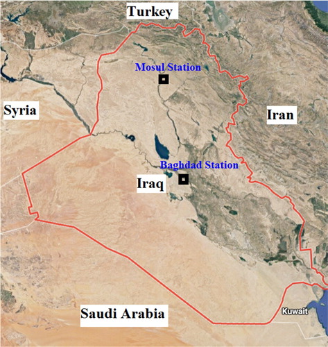
Drought is usually a direct outcome of the balance between precipitation and temperature (Moazenzadeh et al., 2018). The Tigris basin experiences an annual average rainfall ranging between 400 and 600 mm, but it can be as low as 150 mm in the downstream and as high as 800 mm in the upstream in some years. Based on the data from Iraqi meteorological stations, both Baghdad and Mosul have recorded high temperatures over the period from 1999 to 2009. The mean July temperature in Baghdad has ranged from 23.5 to 44.0°C, while the annual rainfall and evaporation rates for the period are 244 and 3200 mm, respectively. Mosul has experienced a mean July temperature range of 24.8 to 43.0°C, with annual precipitation and evaporation rates of 729 and 3900 mm, respectively. Figure 1 shows the location of the meteorological stations.

Figure 1. Map of the selected study locations in Mosul (Station I) and Baghdad (Station II).

3. Applied machine learning models

3.1. CART model

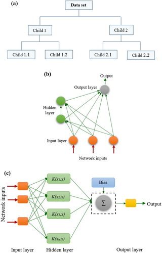
The CART is an ML approach that has been widely used to develop regression and classification models (Breiman, Friedman, Olshen, & Stone, 1984). The CART structure consists of a set of nodes, and each node contains a portion of the data (Kumar, Pandey, Sharma, & Flügel, 2016). A CART model is constructed via recursive partitioning: starting with a single root node, that node is split into left and right child nodes (Pham, Bui, & Prakash, 2018). These child nodes can additionally be split in turn, and themselves become parents of their own child nodes, and so on. Three types of node are used: the root node, the inner nodes, and the terminal nodes. The root node, known as the ‘first parent’, is a parent only, the inner nodes are both children and parents, and the terminal nodes – as the last on their branches – are children only, hence they are also referred to as leaf nodes. All data are included in the root node. Two steps are carried out for each split in the tree: the variable to be used for splitting is selected, then the sets of variable values to be inherited by the left child node and the right child node are defined. The partitioning can then be drawn diagrammatically as a tree (Figure 2(a)).

Figure 2. Model structures for: (a) CART; (b) CCNN; (c) SVM.

3.2. CCNN model

The CCNN (Fahlman & Lebiere, 1990) is a self-organizing network which begins with only input and output neurons. Every input is linked to every output, and each connection is defined by an adjustable weight. From this starting point the network is trained, a process through which neurons are selected from a pool of candidates and added to a hidden layer. One neuron at a time is added to the hidden layer, and once added these neurons do not change. Because the CCNN is self-organizing and grows during the training process, it is not necessary to define the numbers of layers and neurons to be used in the network. Variables are fed into the input layer, which through the weighting in its connections to the output layer along with a constant parallel input known as a bias value uses the neurons in the hidden layer to generate and distribute values into the output layer. The network thus uses feedback from the outputs in conjunction with the neurons in the hidden layer to maximize the correlations while minimizing the residual error. Figure 2(b) presents the cascade architecture.

3.3. GEP model

Gene expression programming (GEP) is an evolutionary learning model introduced by Ferreira (2001) that is made up of chromosomes. The expression tree consists of two parts, the head and the tail, which are encoded in a linear series of fixed-length chromosomes or genomes and then represented as non-linear entities of various shapes and sizes (Ferreira, 2006). Mathematical expressions are automatically represented by a tree expression that consist of nodes containing functions and leaves containing variables and constants. The generated candidates are assessed by using the root relative squared error as a fitness function. The best candidates are then reassessed by applying a modification evaluation cycle until the best solution is achieved. Karva language is used to translate the expression tree by reading it from left to right and from top to bottom. A GEP model is developed using five major steps: (1) identifying the set of independent variables to be utilized in individual programs; (2) defining a set of functions and arithmetic operations; (3) selecting the fitness measure; (4) selecting the head length, the number of genes, and the linking function; and (5) selecting the genetic operators to be used (Ferreira, 2006).

3.4. SVM model

The SVM is a relatively new data-driven method of applied mathematics learning theory that can be used to unravel regression and classification issues (Vapnik, 1995). Classified as a new-generation learning machine, the SVM uses a hyperplane to separate the data from one dimension to high dimensional space and then solves the regression problems using the following equation (Raghavendra & Deka, 2014): (1) $y=f\left(x\right)=\sum _{i=1}^{n}w\times k\left(x_i,x\right)+b,$(1) where w is the weight vector, b is the bias value, and $k\left(x_i,x\right)$ is the kernel function. The values of the internal parameters are determined using the least squares method by minimizing the sum of the squared deviations. The most common regression modeling method in SVM is called -SVM, the cost function for which is formulated as follows: (2) $|\epsilon {|}_{\epsilon }=|y-f\left(x\right){|}_{\epsilon }=\left\{\begin{array}{ll}\epsilon & \text{if}y-f\left(x\right)\le \epsilon \\ |y-f\left(x\right)-\epsilon |& \text{otherwise}\end{array}\right..$(2)

The goal of the cost function is to maximize the ϵ-derivation. The minimization function can be explained as: (3) $Min\frac{1}{2}\parallel w{\parallel }^2+C\left(\sum _i^l{\epsilon }_i^{\ast }+\sum _i^l{\epsilon }_i\right),$(3) which is subject to (4) $\begin{array}{rl}& y_i-w,x-b\le \epsilon +{\epsilon }_i\\ & w,x+b-y_i\le \epsilon +{\epsilon }_i^{\ast }\\ & {\epsilon }_i,{\epsilon }_i^{\ast }\ge 0,\end{array}$(4) where C is the cost factor and ϵ_i and ${\epsilon }_i^{\ast }$ are the slack variables. Linear, polynomial, radial basis, and sigmoid kernel functions can be used in the SVM algorithm. A trial and error technique is employed to select the best kernel function for the specified problem according to the results. In the SVM model the predictors are called attributes, and a hyperplane known as a feature space is used to transform these attributes. The task of selecting the optimum representation is called feature selection, and the set of features that describes a row of predictor values is named a vector. The vectors that are close to the hyperplane are known as support vectors. The model accuracy depends on the choice of optimal parameters for the kernel operation, like C, γ, etc. C is a trade-off between an estimation error and the weight of the vector. The SVM uses the cross-validation method to eliminate overfitting. An example of a traditional SVM network is shown in Figure 2(c).

3.5 Model development

Choosing the appropriate predictors is one of the most important steps in building a robust predictive model (Yaseen, El-shafie, Jaafar, Afan, & Sayl, 2015). In the present study, four different ML models (the CART, the CCNN, GEP, and the SVM) were selected for predicting monthly evaporation. The suggested models were developed using five different input combinations: (5) $\begin{array}{rl}Model1\left(M1\right):E{T}_o& =f\left(WS,RF\right),\end{array}$(5) (6) $\begin{array}{rl}Model2\left(M2\right):E{T}_o& =f\left(WS,RF,RH\right),\end{array}$(6) (7) $\begin{array}{rl}Model3\left(M3\right):E{T}_o& =f\left(WS,RF,RH,T_{\text{min}}\right),\end{array}$(7) (8) $\begin{array}{rl}Model4\left(M4\right):E{T}_o& =f\left(WS,RF,RH,T_{\text{min}},T_{\text{max}}\right),\end{array}$(8) (9) $\begin{array}{rl}Model5\left(M5\right):E{T}_o& =f\left(WS,RF,RH,T_{\text{min}},T_{\text{max}},Sh\right),\end{array}$(9) where ET_o is the evaporation, WS is the wind speed, RF is the rainfall, RH is the relative humidity, T_min is the minimum temperature, T_max is the maximum temperature, and Sh is the number of sunshine hours. The hydrometeorological data were divided into two phases, consisting of 80% training and 20% testing. The data division was performed based on a trial and error procedure through which the best prediction performance was attained. There was no way to anticipate which settings for each proposed model would be needed to obtain the optimum prediction, so several models were developed using a trial and error process and the results of these models were compared in order to select the optimal settings in each case. The GEP model requires the selection of the functions set, population size, genes per chromosomes value, gene head length, fitness function, and linking function, and the genetic operators include the mutation rate, inversion rate, gene transportation rate, one-point recombination rate, two-point recombination rate, gene recombination rate, IS transportation rate, and RIS transportation rate. The SVM model requires the selection of the parameters for the proposed kernel function. The CCNN model requires the selection of the kernel function and the number of hidden neurons that are created during the training process. The CART model requires the selection of the minimum number of rows per node, the minimum size node that can be split, and the maximum number of tree levels. The predictive modeling software DTREG was used to develop the models in this study (Sherrod, 2003).

3.6. Prediction performance metrics

The performance of the predictive models was assessed using the following statistical metrics: the root mean square error (RMSE), the mean absolute error (MAE), the Nash–Sutcliffe coefficient (NSE), Willmott’s Index (WI), Legate and McCabe’s Index (LMI), and the determination coefficient (R²) (Chai & Draxler, 2014; Legates & McCave, 1999). The mathematical expressions of the performance metrics are as follows: (10) $\begin{array}{rl}RMSE& =\sqrt{\frac{1}{N}\sum _{t=1}^n{\left(ET{o}_{obs}-ET{o}_{pred}\right)}^2}\left[0,+\mathrm{\infty }\right],\end{array}$(10) (11) $\begin{array}{rl}MAE& =\frac{1}{N}\sum _{t=1}^n|ET{o}_{obs}-ET{o}_{pred}|\left[0,+\mathrm{\infty }\right],\end{array}$(11) (12) $\begin{array}{rl}NSE& =1-\left[\frac{{\sum }_{i=1}^N{\left(ET{o}_{obs}-ET{o}_{pred}\right)}^2}{{\sum }_{i=1}^N{\left(ET{o}_{obs}-\overline{ET{o}_{pred}}\right)}^2}\right]\left[-\mathrm{\infty },1\right],\end{array}$(12) (13) $\begin{array}{rl}WI& =1-\left[\frac{{\sum }_{i=1}^N{\left(W{L}_{obs}-W{L}_{pred}\right)}^2}{\begin{array}{c}{\sum }_{i=1}^N(|ET{o}_f-\overline{ET{o}_o}|\\ {+|ET{o}_o-\overline{ET{o}_o}|)}^2\end{array}}\right]\left[0,1\right],\end{array}$(13) (14) $\begin{array}{rl}LMI& =1-\left[\frac{{\sum }_{i=1}^N|ET{o}_{obs}-ET{o}_{pred}|}{{\sum }_{i=1}^N|ET{o}_{obs}-\overline{ET{o}_{obs}}|}\right]\left[-\mathrm{\infty },1\right],\end{array}$(14) (15) $\begin{array}{rl}{R}^2& ={\left(\frac{\begin{array}{c}{\sum }_{i=1}^N\left(ET{o}_{obs}-\overline{ET{o}_{obs}}\right)\\ \left(ET{o}_{pred}-\overline{ET{o}_{pred}}\right)\end{array}}{\sqrt{\begin{array}{c}{\sum }_{i=1}^N{\left(W{L}_{obs}-\overline{W{L}_{obs}}\right)}^2\\ {\sum }_{i=1}^N{\left(W{L}_{pred}-\overline{W{L}_{pred}}\right)}^2\end{array}}}\right)}^2\left[0,1\right],\end{array}$(15) where $ET{o}_{obs}$ and $ET{o}_{pred}$ are the observed and predicted evaporation processes, and $\overline{ET{o}_{obs}}$ and $\overline{ET{o}_{pred}}$ are the mean values of the observed and predicted evaporation processes.

4. Application and analysis

The performance of the four constructed ML models was tested by predicting evaporation at two different meteorological stations in Iraq. Station I (in Mosul) is located in a semi-arid environment, whereas Station II (in Baghdad) is located in an arid environment. Evaporation was predicted using five different input combinations of related meteorological variables (M1, M2, M3, M4, and M5).

The performance of the four ML models during the training and testing phases at Station I in Mosul is given in Tables 1Table 2.Table 3.–4. The results show that during training the CCNN model produced the most accurate prediction with the lowest RMSE (23.83 mm.d⁻¹) and the highest R² (.97) using only the three input variables of wind speed, rainfall, and relative humidity. However, in general, the best prediction capacity is attained when all the input variables are used for the prediction matrix (the M5 input combination). This is clearly evidenced in the high correlation of evaporation with different climate variables such as wind speed, rainfall, sunshine hours, humidity, and air temperature. The second best model during the training process was the CART model, with the lowest RMSE (33.33 mm.d⁻¹) and the highest R² (.94) for the M5 input combination. During the testing phase, all four models attained their best performances for the M2 input combination, wherein just the wind speed, rainfall, and relative humidity are used. The results also show that the CCNN model performed best on all the metrics during the training phase, and the other three models tended to produce performances that were relatively similar to each other. However, the CART, GEP, and SVM models produced very similar results for all the performance metrics during the testing phase for the M2 input combination, and their performance was found to be better than that of the CCNN model in this phase.

Table 1. The statistical performance metrics of the applied CART model over the training and testing phases at Station I in Mosul.

Model	Performance metrics
	Training phase
	RMSE	MAE	NSE	WI	LMI	R^2
M1	70.81	52.39	.75	.92	.56	.75
M2	53.11	37.42	.85	.96	.68	.85
M3	51.31	35.42	.86	.96	.70	.86
M4	48.35	31.38	.88	.96	.73	.88
M5	33.33	21.68	.94	.98	.82	.94
	Testing phase
M1	67.70	51.34	.71	.92	.53	.80
M2	36.35	30.54	.91	.97	.72	.93
M3	91.89	56.65	.46	.86	.48	.58
M4	58.09	41.43	.78	.94	.62	.86
M5	48.89	37.61	.84	.96	.65	.87

Note: LMI = Legate and McCabe’s Index; MAE = mean absolute error; NSE = Nash–Sutcliffe coefficient; R² = determination coefficient; RMSE = root mean square error; WI = Willmott’s Index. Bold font denotes lowest RMSE value in each phase.

Table 2. The statistical performance metrics of the applied CCNN model over the training and testing phases at Station I in Mosul.

Model	Performance metrics
	Training phase
	RMSE	MAE	NSE	WI	LMI	R^2
M1	41.67	20.38	.91	.97	.83	.91
M2	23.82	8.58	.97	.99	.92	.97
M3	44.81	29.81	.90	.97	.75	.90
M4	46.15	29.54	.89	.97	.75	.89
M5	45.78	29.71	.89	.97	.75	.89
	Testing phase
M1	91.22	69.43	.48	.87	.36	.62
M2	52.64	40.12	.81	.95	.63	.86
M3	68.05	44.27	.70	.92	.59	.74
M4	68.05	44.27	.70	.92	.59	.74
M5	74.17	42.19	.64	.91	.61	.69

Note: LMI = Legate and McCabe’s Index; MAE = mean absolute error; NSE = Nash–Sutcliffe coefficient; R² = determination coefficient; RMSE = root mean square error; WI = Willmott’s Index. Bold font denotes lowest RMSE value in each phase.

Table 3. The statistical performance metrics of the applied GEP model over the training and testing phases at Station I in Mosul.

Model	Performance metrics
	Training phase
	RMSE	MAE	NSE	WI	LMI	R^2
M1	70.81	52.39	.75	.92	.56	.75
M2	53.11	37.42	.85	.96	.68	.85
M3	51.31	35.42	.86	.96	.70	.86
M4	48.35	31.38	.88	.96	.73	.88
M5	44.46	28.66	.90	.97	.76	.90
	Testing phase
M1	67.70	51.34	.71	.92	.53	.80
M2	36.35	30.54	.91	.97	.72	.93
M3	91.89	56.65	.46	.86	.48	.58
M4	58.09	41.43	.78	.94	.62	.86
M5	61.03	37.94	.75	.93	.65	.79

Note: LMI = Legate and McCabe’s Index; MAE = mean absolute error; NSE = Nash–Sutcliffe coefficient; R² = determination coefficient; RMSE = root mean square error; WI = Willmott’s Index. Bold font denotes lowest RMSE value in each phase.

Table 4. The statistical performance metrics of the applied SVM model over the training and testing phases at Station I in Mosul.

Model	Performance metrics
	Training phase
	RMSE	MAE	NSE	WI	LMI	R^2
M1	68.14	47.34	.76	.92	.60	.77
M2	51.01	33.40	.87	.96	.72	.87
M3	51.01	33.40	.87	.96	.72	.87
M4	47.72	31.37	.88	.96	.73	.89
M5	45.23	27.44	.89	.97	.77	.90
	Testing phase
M1	61.15	47.88	.76	.93	.56	.80
M2	35.76	27.71	.91	.97	.74	.92
M3	73.41	40.10	.64	.90	.63	.69
M4	73.41	40.10	.64	.90	.63	.69
M5	58.20	33.77	.77	.94	.69	.79

Note: LMI = Legate and McCabe’s Index; MAE = mean absolute error; NSE = Nash–Sutcliffe coefficient; R² = determination coefficient; RMSE = root mean square error; WI = Willmott’s Index. Bold font denotes lowest RMSE value in each phase.

For Station II in Baghdad, all the applied ML models achieved their best performance during both the training and testing phases when the M5 input combination was used (Tables 5Table 6.Table 7.–8). The results show that the CART performed better than the other three models during the training phase, whereas the SVM performed the best during the testing phase. In terms of the statistical metrics, the SVM yielded the lowest RMSE (32.27 mm.d⁻¹) and the highest R² (.97).

Table 5. The statistical performance metrics of the applied CART model over the training and testing phases at Station II in Baghdad.

Model	Performance metrics
	Training phase
	RMSE	MAE	NSE	WI	LMI	R^2
M1	40.11	28.52	.94	.98	.81	.94
M2	44.13	32.13	.93	.98	.79	.93
M3	36.68	25.48	.95	.98	.83	.95
M4	32.95	23.46	.96	.99	.84	.96
M5	31.06	21.27	.96	.99	.86	.96
	Testing phase
M1	86.04	65.10	.72	.92	.55	.74
M2	65.18	46.93	.84	.95	.67	.85
M3	53.76	40.03	.89	.97	.72	.92
M4	51.22	39.10	.90	.97	.73	.92
M5	49.38	36.81	.91	.97	.74	.94

Note: LMI = Legate and McCabe’s Index; MAE = mean absolute error; NSE = Nash–Sutcliffe coefficient; R² = determination coefficient; RMSE = root mean square error; WI = Willmott’s Index. Bold font denotes lowest RMSE value in each phase.

Table 6. The statistical performance metrics of the applied CCNN model over the training and testing phases at Station II in Baghdad.

Model	Performance metrics
	Training phase
	RMSE	MAE	NSE	WI	LMI	R^2
M1	73.54	56.31	.82	.95	.63	.82
M2	52.19	39.66	.91	.97	.74	.91
M3	46.73	34.53	.93	.98	.77	.93
M4	46.36	34.60	.93	.98	.77	.93
M5	43.37	32.01	.94	.98	.79	.94
	Testing phase
M1	84.29	66.87	.73	.92	.53	.74
M2	57.46	45.78	.87	.96	.68	.89
M3	50.30	37.84	.90	.97	.73	.95
M4	47.49	37.92	.91	.97	.73	.95
M5	37.88	29.63	.94	.98	.79	.96

Note: LMI = Legate and McCabe’s Index; MAE = mean absolute error; NSE = Nash–Sutcliffe coefficient; R² = determination coefficient; RMSE = root mean square error; WI = Willmott’s Index. Bold font denotes lowest RMSE value in each phase.

Table 7. The statistical performance metrics of the applied GEP model over the training and testing phases at Station II in Baghdad.

Model	Performance metrics
	Training phase
	RMSE	MAE	NSE	WI	LMI	R^2
M1	83.38	65.69	.78	.93	.57	.78
M2	67.89	54.33	.85	.95	.64	.85
M3	67.89	54.33	.85	.95	.64	.85
M4	45.93	33.55	.93	.98	.78	.93
M5	45.94	33.91	.93	.98	.78	.93
	Testing phase
M1	83.45	70.18	.74	.92	.51	.74
M2	64.84	53.94	.84	.95	.62	.89
M3	54.58	43.09	.89	.97	.70	.95
M4	48.10	36.64	.91	.98	.74	.96
M5	36.63	28.80	.94	.98	.80	.95

Note: LMI = Legate and McCabe’s Index; MAE = mean absolute error; NSE = Nash–Sutcliffe coefficient; R² = determination coefficient; RMSE = root mean square error; WI = Willmott’s Index. Bold font denotes lowest RMSE value in each phase.

Table 8. The statistical performance metrics of the applied SVM model over the training and testing phases at Station II in Baghdad.

Model	Performance metrics
	Training phase
	RMSE	MAE	NSE	WI	LMI	R^2
M1	80.82	59.77	.79	.94	.61	.79
M2	52.86	37.47	.91	.97	.75	.91
M3	52.86	37.47	.91	.97	.75	.91
M4	40.11	28.52	.94	.98	.81	.94
M5	41.34	28.29	.94	.98	.81	.94
	Testing phase
M1	81.74	66.42	.75	.92	.54	.75
M2	55.49	41.22	.88	.97	.71	.89
M3	45.38	34.03	.92	.98	.76	.95
M4	43.78	32.69	.92	.98	.77	.93
M5	32.27	24.75	.96	.99	.82	.97

Note: LMI = Legate and McCabe’s Index; MAE = mean absolute error; NSE = Nash–Sutcliffe coefficient; R² = determination coefficient; RMSE = root mean square error; WI = Willmott’s Index. Bold font denotes lowest RMSE value in each phase.

Overall, the results from the two stations indicate that the applied ML models achieved their best performance in terms of the six metrics when all the climatological information was incorporated, i.e. for the M5 input combination. In other words, the results demonstrate that the performance of these models increases as the number of inputs into the models increases. Moreover, when comparing the results of the performance metrics from both stations, the ML models tend to produce different results for different stations, which indicates that the model performance also depends on the climate of the investigated area.

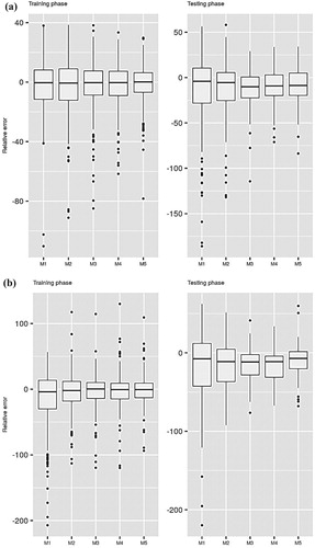
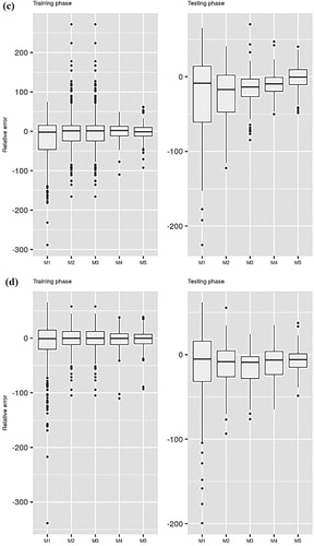
Figures 3 and 4 present box plots of the relative errors computed for Stations I and II, respectively. The figures show that the performances differ based on the employed ML model, the input combinations, and the locations. Higher relative errors are obtained when the minimum number of inputs is used for constructing the predictive models. The error decreases exponentially as the number of inputs increases, which further supports the tabulated results presented above.

Figure 3. Relative error performance of the applied predictive models at Station I: (a) CART; (b) CCNN; (c) GEP; (d) SVM.

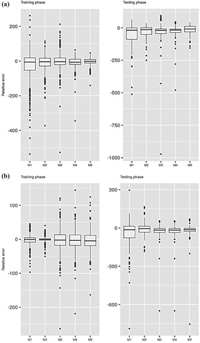
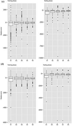
Figure 4. Relative error performance of the applied predictive models at Station II: (a) CART; (b) CCNN; (c) GEP; (d) SVM.

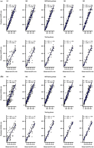
Scatter plots are also used to compare the performance of the ML models (Figures 5 and 6). The plots show the agreement between the observed and predicted evaporation using the determination coefficient (R²) and the slope of the regression model. Generally, the results show that all the models have the highest R² for the M5 input combination, and the regression models best fit the predicted observations for that combination.

Figure 5. Scatter plot performance of the applied predictive models at Station I: (a) CART; (b) CCNN; (c) GEP; (d) SVM.

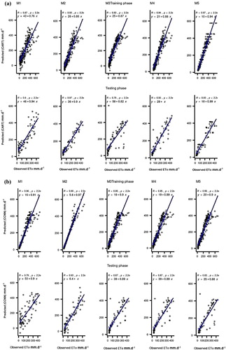
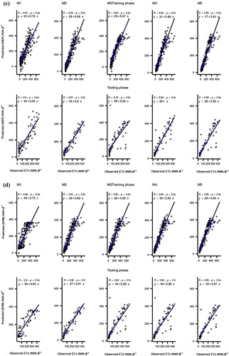
Figure 5. Scatter plot performance of the applied predictive models at Station II: (a) CART; (b) CCNN; (c) GEP; (d) SVM.

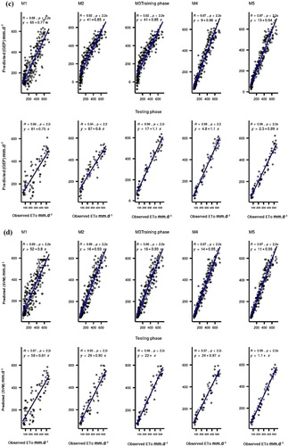
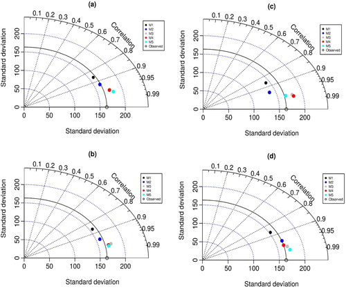
Figures 7 and 8 exhibit the performance of the ML models at Stations I and II, respectively, through Taylor diagrams. The figures show a statistical summary of the predicted and observed evaporation in accordance with several statistical metrics, including the RMSE, standard deviations, and correlation coefficients. The results here demonstrate the superiority of the SVM model over the other applied models.

Figure 7. Taylor diagram visualizations for the performance of the applied predictive models at Station I: (a) CART; (b) CCNN; (c) GEP; (d) SVM.

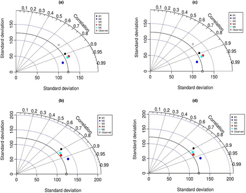
Figure 8. Taylor diagram visualizations for the performance of the applied predictive models at Station II: (a) CART; (b) CCNN; (c) GEP; (d) SVM.

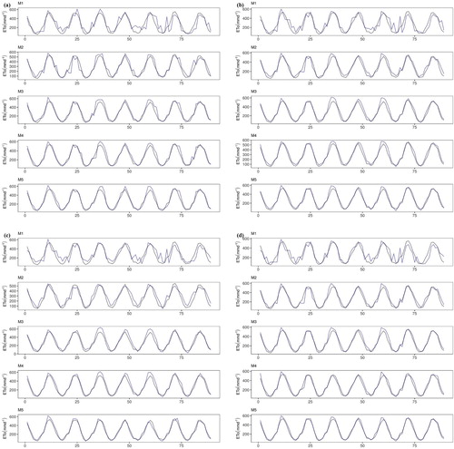
Finally, the observed and predicted evaporation are plotted as time series in Figures 9 and 10 for Stations I and II, respectively. The black and dark blue lines in the figures denote the observed and predicted time series, respectively. It can be clearly seen that the predicted series fluctuate more compared to the observed series when a lower number of input variables is used for the development of the models, whereas the predicted series completely overlap the observed series when all the meteorological variables are used as inputs.

Figure 9. Time series data visualization between the performance of the applied predictive models (dark blue lines) and the observed evaporation process (black lines) at Station I: (a) CART; (b) CCNN; (c) GEP; (d) SVM.

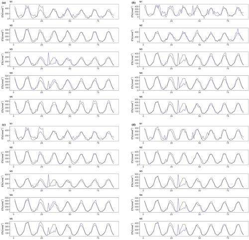
Figure 10. Time series data visualization between the performance of the applied predictive models (dark blue lines) and the observed evaporation process (black lines) at Station II: (a) CART; (b) CCNN; (c) GEP; (d) SVM.

Overall, these findings demonstrate that the applied ML models produce more accurate results when a full set of meteorological information is used. The predictive performances vary for the different methods used for the development of the models. Overall, the SVM achieves the most accurate prediction performance for most of the cases. It is also important to note that the performance of the models differs according to the climate of the investigated region.

5. Conclusion

The prediction of evaporation is one of the most complex tasks in hydrological engineering. In nature, evaporation is associated with multiple climate variables and thus is characterized by high non-linearity and stochasticity. For a developing country like Iraq, evaporation monitoring and measurement is limited due to the non-maintained meteorological stations. Thus, the introduction of ML technologies can contribute greatly by better modeling this hydrological process. Four different versions of ML models – the CART, the CCNN, GEP, and the SVM – were developed for the prediction of evaporation at two meteorological stations in Iraq located in different climates, Station I in Mosul and Station II in Baghdad. Overall, the applied ML models demonstrate high performance in simulating evaporation for both arid and semi-arid climates. Among the four ML models, the SVM exhibits superior prediction performance. In quantitative terms, at Station I, M2 was the best input combination for the SVM, yielding an RMSE of 35.76 mm.d⁻¹, an MAE of 27.71 mm.d⁻¹, and an R² of .92 during testing. At Station II, M5 was the best input combination for the SVM, yielding an RMSE of 32.27 mm.d⁻¹, an MAE of 24.75 mm.d⁻¹, and an R² of .97 during testing. Based on the attained prediction results, the predictive model demonstrated better accuracy at Baghdad Station. This can be justified due to the high climate stochasticity at Mosul Station. Further work is needed to assess the uncertainty in prediction due to the model structures and input combinations.

Acknowledgments

The authors would like to acknowledge the data source providers, the Meteorological Organization of Seismology (MOS) and the Ministry of Agriculture and Water Resources of Iraq. The editors and reviewers are very much appreciated for their constructive comments.

Disclosure statement

No potential conflict of interest was reported by the authors.

References

- Abbas, N., Wasimi, S. A., Al-Ansari, N., & Sultana, N. (2018). Water resources problems of Iraq: Climate change adaptation and mitigation. Journal of Environmental Hydrology, 26(6), 1–6. Retrieved from http://www.diva-portal.org/smash/get/diva2:1206419/FULLTEXT01.pdf
- Abdullah, S. S., Malek, M. A., Abdullah, N. S., Kisi, O., & Yap, K. S. (2015). Extreme learning machines: A new approach for prediction of reference evapotranspiration. Journal of Hydrology, 527, 184–195. doi: 10.1016/j.jhydrol.2015.04.073
- Abghari, H., Ahmadi, H., Besharat, S., & Rezaverdinejad, V. (2012). Prediction of daily pan evaporation using wavelet neural networks. Water Resources Management, 26(12), 3639–3652. doi: 10.1007/s11269-012-0096-z
- Al-Ansari, N., Ali, A. A., & Knutsson, S. (2014). Present conditions and future Challenges of water resources problems in Iraq. Journal of Water Resource and Protection, 6, 1066–1098. doi: 10.4236/jwarp.2014.612102
- Al-Taai, O. T., & Hadi, S. H. (2018). Analysis of the monthly and annual change of soil Moisture and evaporation in Iraq. Al-Mustansiriyah Journal of Science, 29(4), 7–13.
- Ali Ghorbani, M., Kazempour, R., Chau, K.-W., Shamshirband, S., & Taherei Ghazvinei, P. (2018). Forecasting pan evaporation with an integrated artificial neural network quantum-behaved particle swarm optimization model: A case study in Talesh, Northern Iran. Engineering Applications of Computational Fluid Mechanics, 12(1), 724–737. doi: 10.1080/19942060.2018.1517052
- Baydarolu, Ö, & Koçak, K. (2014). SVR-based prediction of evaporation combined with chaotic approach. Journal of Hydrology, 508, 356–363. doi: 10.1016/j.jhydrol.2013.11.008
- Boers, T. M., De Graaf, M., Feddes, R. A., & Ben-Asher, J. (1986). A linear regression model combined with a soil water balance model to design micro-catchments for water harvesting in arid zones. Agricultural Water Management, doi: 10.1016/0378-3774(86)90038-7
- Breiman, L., Friedman, J. H., Olshen, R. A., & Stone, C. J. (1984). Classification and regression trees. The Wadsworth statisticsprobability series (Vol. 19). doi: 10.1371/journal.pone.0015807
- Chai, T., & Draxler, R. R. (2014). Root mean square error (RMSE) or mean absolute error (MAE)? Arguments against avoiding RMSE in the literature. Geoscientific Model Development, 7(3), 1247–1250. doi: 10.5194/gmd-7-1247-2014
- Chenoweth, J., Hadjinicolaou, P., Bruggeman, A., Lelieveld, J., Levin, Z., Lange, M. A., … Hadjikakou, M. (2011). Impact of climate change on the water resources of the eastern Mediterranean and Middle East region: Modeled 21st century changes and implications. Water Resources Research, doi: 10.1029/2010WR010269
- Danandeh Mehr, A., Nourani, V., Kahya, E., Hrnjica, B., Sattar, A. M. A., & Yaseen, Z. M. (2018). Genetic programming in water resources engineering: A state-of-the-art review. Journal of Hydrology, doi: 10.1016/j.jhydrol.2018.09.043
- Di, N., Wang, Y., Clothier, B., Liu, Y., Jia, L., Xi, B., & Shi, H. (2019). Modeling soil evaporation and the response of the crop coefficient to leaf area index in mature Populus tomentosa plantations growing under different soil water availabilities. Agricultural and Forest Meteorology, doi: 10.1016/j.agrformet.2018.10.004
- Eames, I. W., Marr, N. J., & Sabir, H. (1997). The evaporation coefficient of water: A review. International Journal of Heat and Mass Transfer, doi: 10.1016/S0017-9310(96)00339-0
- Fahimi, F., Yaseen, Z. M., & El-shafie, A. (2016). Application of soft computing based hybrid models in hydrological variables modeling: A comprehensive review. Theoretical and Applied Climatology, 1–29. doi: 10.1007/s00704-016-1735-8
- Fahlman, S. E., & Lebiere, C. (1990). The cascade-correlation learning architecture. Advances in Neural Information Processing Systems, 524–532. doi: 10.1190/1.1821929
- Fallah-Mehdipour, E., Bozorg Haddad, O., & Mariño, M. A. (2013). Prediction and simulation of monthly groundwater levels by genetic programming. Journal of Hydro-Environment Research, 7(4), 253–260. doi: 10.1016/j.jher.2013.03.005
- Ferreira, C. (2001). Gene expression programming: A new adaptive algorithm for solving problems. Complex Systems, 13(2), 1–22. Retrieved from http://arxiv.org/abs/cs/0102027
- Ferreira, C. (2006). Gene expression programming: Mathematical modeling by an artificial intelligence (2nd). Berlin: Springer.
- Fotovatikhah, F., Herrera, M., Shamshirband, S., Ardabili, S. F., & Piran, J. (2018). Survey of computational intelligence as basis to big flood management: Challenges, research directions and future work. Engineering Applications of Computational Fluid Mechanics, 12(1), 411–437. doi: 10.1080/19942060.2018.1448896
- Ghorbani, M. A., Deo, R. C., Karimi, V., Yaseen, Z. M., & Terzi, O. (2017). Implementation of a hybrid MLP-FFA model for water level prediction of Lake Egirdir, Turkey. Stochastic Environmental Research and Risk Assessment, 1–15. doi: 10.1007/s00477-017-1474-0
- Jing, W., Yaseen, Z. M., Shahid, S., Saggi, M. K., Tao, H., Kisi, O., … Chau, K.-W. (2019). Implementation of evolutionary computing models for reference evapotranspiration modeling: Short review, assessment and possible future research directions. Engineering Applications of Computational Fluid Mechanics, 13(1), 811–823. doi: 10.1080/19942060.2019.1645045
- Khan, N., Shahid, S., Ismail, T. B., & Wang, X.-J. (2018). Spatial distribution of unidirectional trends in temperature and temperature extremes in Pakistan. Theoretical and Applied Climatology, 136(3–4), 899–913. doi: 10.1007/s00704-018-2520-7
- Khan, N., Shahid, S., Juneng, L., Ahmed, K., Ismail, T., & Nawaz, N. (2019). Prediction of heat waves in Pakistan using quantile regression forests. Atmospheric Research, doi: 10.1016/j.atmosres.2019.01.024
- Kumar, D., Pandey, A., Sharma, N., & Flügel, W. A. (2016). Daily suspended sediment simulation using machine learning approach. Catena, doi: 10.1016/j.catena.2015.11.013
- Legates, D. R., & McCave Jr., G. J. (1999). Evaluating the use of ‘goodness-of-fit’ measures in hydrologic and hydroclimatic model validation. Water Resources Research, 35(1), 233–241. doi: 10.1029/1998WR900018
- Lelieveld, J., Hadjinicolaou, P., Kostopoulou, E., Chenoweth, J., El Maayar, M., Giannakopoulos, C., … Xoplaki, E. (2012). Climate change and impacts in the Eastern Mediterranean and the Middle East. Climatic Change, doi: 10.1007/s10584-012-0418-4
- Lu, X., Ju, Y., Wu, L., Fan, J., Zhang, F., & Li, Z. (2018). Daily pan evaporation modeling from local and cross-station data using three tree-based machine learning models. Journal of Hydrology, 566, 668–684. doi: 10.1016/j.jhydrol.2018.09.055
- Majhi, B., Naidu, D., Mishra, A. P., & Satapathy, S. C. (2019). Improved prediction of daily pan evaporation using deep-LSTM model. Neural Computing and Applications, doi: 10.1007/s00521-019-04127-7
- Moazenzadeh, R., Mohammadi, B., Shamshirband, S., & Chau, K. (2018). Coupling a firefly algorithm with support vector regression to predict evaporation in northern Iran. Engineering Applications of Computational Fluid Mechanics, 12(1), 584–597. doi: 10.1080/19942060.2018.1482476
- Moran, M. S., Rahman, A. F., Washburne, J. C., Goodrich, D. C., Weltz, M. A., & Kustas, W. P. (1996). Combining the Penman-Monteith equation with measurements of surface temperature and reflectance to estimate evaporation rates of semiarid grassland. Agricultural and Forest Meteorology, doi: 10.1007/s12549-010-0046-9
- Penman, H. L. (1948). Natural evaporation from open water, bare soil and grass. Proceedings of the Royal Society of London. Series A: Mathematical and Physical Sciences, 193(1032), 120–145. doi: 10.1098/rspa.1948.0037
- Pham, B. T., Bui, D. T., & Prakash, I. (2018). Application of classification and regression trees for spatial prediction of rainfall-induced shallow landslides in the Uttarakhand area (India) using GIS. In Climate change, extreme events and disaster risk reduction (pp. 159–170). Cham: Springer.
- Priestley, C. H. B., & Taylor, R. J. (1972). On the assessment of the surface heat flux and evaporation using large-scale parameters. Monthly Weather Review, 100, 81–92. doi: 10.1175/1520-0493(1972)100<0081:OTAOSH>2.3.CO;2
- Qasem, S. N., Samadianfard, S., Kheshtgar, S., Jarhan, S., Kisi, O., Shamshirband, S., & Chau, K.-W. (2019). Modeling monthly pan evaporation using wavelet support vector regression and wavelet artificial neural networks in arid and humid climates. Engineering Applications of Computational Fluid Mechanics, doi: 10.1080/19942060.2018.1564702
- Raghavendra, S., & Deka, P. C. (2014). Support vector machine applications in the field of hydrology: A review. Applied Soft Computing, 19, 372–386. doi: 10.1016/j.asoc.2014.02.002
- Sartori, E. (2000). A critical review on equations employed for the calculation of the evaporation rate from free water surfaces. Solar Energy, doi: 10.1016/S0038-092X(99)00054-7
- Sayl, K. N., Muhammad, N. S., Yaseen, Z. M., & El-shafie, A. (2016). Estimation the physical variables of rainwater harvesting system using integrated GIS-based remote sensing approach. Water Resources Management, 30(9), 3299–3313. doi: 10.1007/s11269-016-1350-6
- Sherrod, P. H. (2003). DTREG predictive modeling software. Software. Retrieved from http://www.dtreg.com
- Stanhill, G. (2002). Is the class a evaporation pan still the most practical and accurate meteorological method for determining irrigation water requirements? Agricultural and Forest Meteorology, doi: 10.1016/S0168-1923(02)00132-6
- Stewart, J. B. (1984). Measurement and prediction of evaporation from forested and agricultural catchments. In Developments in agricultural and managed forest ecology (Vol. 13, pp. 1–28). New York: Elsevier.
- Tabari, H., Marofi, S., & Sabziparvar, A. A. (2010). Estimation of daily pan evaporation using artificial neural network and multivariate non-linear regression. Irrigation Science, 28(5), 399–406. doi: 10.1007/s00271-009-0201-0
- Vapnik, V. (1995). The nature of statistical learning theory. Data mining and knowledge discovery. Retrieved from http://infoscience.epfl.ch/record/82790/files/com02-04.pdf
- Yaseen, Z. M., El-shafie, A., Jaafar, O., Afan, H. A., & Sayl, K. N. (2015). Artificial intelligence based models for stream-flow forecasting: 2000–2015. Journal of Hydrology, 530, 829–844. doi: 10.1016/j.jhydrol.2015.10.038
- Yaseen, Z. M., Ramal, M. M., Diop, L., Jaafar, O., Demir, V., & Kisi, O. (2018). Hybrid adaptive neuro-fuzzy models for water quality index estimation. Water Resources Management, doi: 10.1007/s11269-018-1915-7
- Yaseen, Z. M., Sulaiman, S. O., Deo, R. C., & Chau, K.-W. (2019). An enhanced extreme learning machine model for river flow forecasting: State-of-the-art, practical applications in water resource engineering area and future research direction. Journal of Hydrology, 569, 387–408. doi: 10.1016/j.jhydrol.2018.11.069