Two-dimensional smoothed particle hydrodynamics (SPH) simulation of multiphase melting flows and associated interface behavior

ABSTRACT

Heat transfer and phase change in multiphase media involve complex behavior such as multi-physics coupling, unsteady interfaces, and boundary generation/disappearance. The smoothed particle hydrodynamics (SPH) method is used to simulate multicomponent problems (initially solid material surrounded by a fluid) characterized by heat transfer, solid–liquid phase change, and multiphase flow. First, the interface behavior of the melted liquids and ambient fluids are simulated by a multiphase SPH model, where corrected algorithms and techniques are adopted to provide a stable simulation for the interface with a large density ratio. The wetting effect of the solid surface by melted liquids is considered by extending the continuum surface force model to three phases including solid, melted liquid and ambient fluid. Second, a thermal dynamics model is incorporated with the multiphase SPH model. The solid–liquid phase change occurs in a small temperature interval in which the latent heat is incorporated using the equivalent heat capacity. Third, the numerical model is validated using several benchmark examples. Five specially configured cases are simulated to demonstrate the robustness, adaptability, and stability of the model. The intriguing phenomena of evolution of the fluid interface of melted liquids, accumulation of thin-layer liquids, and melted droplet formation are reproduced.

KEYWORDS:

• Smoothed particle hydrodynamics
• multiphase flow
• thermal dynamics
• solid–liquid phase change
• unsteady interface behavior

List of notation

c	=	sound speed, m/s
$c_l$	=	sound speed of heavy phase, m/s
$c_g$	=	sound speed of light phase, m/s
$c_{0l}$	=	reference sound speed of heavy phase, m/s
$c_{0g}$	=	reference sound speed of light phase, m/s
$c_p$	=	heat capacity, J/(kg·°C)
$c_{pl}$	=	heat capacity of the liquid, J/(kg·°C)
$c_{pm}$	=	heat capacity of the material in phase change, J/(kg·°C)
$c_{ps}$	=	heat capacity of the solid, J/(kg·°C)
$c_i^j$, $c_i^i$	=	color function
$\mathrm{\nabla }{c}_i$	=	gradient of color function
g	=	gravity acceleration, m/s2
h	=	smoothing length, m
i	=	particle i
j	=	particle j
k	=	thermal conductivity, W/(m·°C)
$k_i$	=	thermal conductivity of particle i, W/(m·°C)
$k_j$	=	thermal conductivity of particle j, W/(m·°C)
$m_i$	=	mass of particle i, kg
$m_j$	=	mass of particle j, kg
${\mathit{n}}_{\mathit{i}}$	=	unit normal vector of particle i
${\mathit{n}}_{\mathit{i}}^{f_2-s}$	=	unit normal vector of particle i at the interface between Fluid 2 and solid
${\mathit{n}}_{\mathit{i}}^{f_2-f_1}$	=	unit normal vector of particle i at the interface between Fluid 2 and Fluid 1
p	=	pressure, Pa
$p_b$	=	background pressure, Pa
$p_i$	=	pressure of particle i, Pa
$p_j$	=	pressure of particle j, Pa
$p_g$	=	pressure of light phase, Pa
$p_l$	=	pressure of heavy phase, Pa
${\dot{q}}_s^{\ast }$	=	volumetric heat source, W/(m3)
${\dot{q}}_l^{\ast }$	=	volumetric heat loss, W/(m3)
t	=	time, s
$\mathrm{\Delta }t$	=	integral time step, s
$\mathrm{\Delta }{t}_c$	=	integral time step constrained by inertia, s
$\mathrm{\Delta }{t}_{surf}$	=	integral time step constrained by surface tension, s
$\mathrm{\Delta }{t}_{visc}$	=	integral time step constrained by viscosity, s
$\mathrm{\Delta }{t}_T$	=	integral time step constrained by thermal field, s
$\mathit{v}$	=	velocity vector, m/s
vb	=	characteristic velocity, m/s
Δx	=	initial particle spacing, m
$C_0$, $C_1$	=	coefficient of Gaussian kernel function
${\mathit{F}}^S$	=	surface tension force per unit mass, N/kg.
${\mathit{F}}_i^{f_2-s}$	=	component of surface tension force on particle i at the interface between Fluid 2 and solid, N/kg.
${\mathit{F}}_i^{f_2-f_1}$	=	component of surface tension force on particle i at the interface between Fluid 1 and Fluid 2, N/kg.
${\mathit{F}}^B$	=	body force per unit mass, N/kg.
${\mathit{F}}^{interface}$	=	interface sharpness force, N/kg
L	=	latent heat, J/kg
$L_0$	=	maximum depth of still water, m
Ma	=	Mach number
$N_i$	=	number of neighboring particles of particle i
R	=	characteristic length or bubble radius, m
S	=	position of the solid–liquid interface, m
T	=	temperature, °C
Tm	=	melting temperature, °C
$\mathrm{\Delta }T$	=	temperature interval of phase change, °C
$U_{max}$	=	maximum velocity, m/s
$V_i$, $V_j$	=	volume of the particles i and j, m3
W	=	abbreviation of kernel function $W\left(\mathit{x}-{\mathit{x}}^{\mathbf{\prime }},h\right)$
$\mathrm{\nabla }W$	=	abbreviation of gradient of kernel function ${\mathrm{\nabla }}_{\mathit{x}}W\left(\mathit{x}-{\mathit{x}}^{\mathbf{\prime }},h\right)$
$\alpha$	=	coefficient for scaling background pressure
$\gamma$	=	EOS constant
${\gamma }_g$	=	EOS constant for light phase
${\gamma }_l$	=	EOS constant for heavy phase
$ϵ$	=	parameter for scaling the smoothing length
$\zeta$	=	constant for interface sharpness force (Equation (49))
θeq	=	static contact angle, °
θd	=	dynamic contact angle, °
$\vartheta$	=	relative change rate of the fluid density denoting the degree of compressibility of fluid
$\lambda$	=	weight function in surface tension force equation
${\lambda }_s$	=	coefficient in the analytical solution of interface position for Stefan problem
$\mu$	=	dynamic viscosity, N·s/m2
${\mu }_i$	=	dynamic viscosity of particle i, N·s/m2
${\mu }_j$	=	dynamic viscosity of particle j, N·s/m2
${\mu }_{ij}$	=	harmonic mean of ${\mu }_i$ and ${\mu }_j$
${\xi }_i$	=	curvature of interface particle i, 1/m
ρ	=	density, kg/m3
${\rho }_{f1}$	=	density of Fluid 1, kg/m3
${\rho }_{f2}$	=	density of Fluid 2, kg/m3
${\rho }_i$	=	density of particle i, kg/m3
${\rho }_0$	=	reference density, kg/m3
${\rho }_{0g}$	=	reference density of light phase, kg/m3
${\rho }_{0l}$	=	reference density of heavy phase, kg/m3
$\sigma$	=	surface tension coefficient, N/m
${\sigma }^{f_2-s}$	=	surface tension coefficient between Fluid 2 and solid, N/m
${\sigma }^{f_2-f_1}$	=	surface tension coefficient between Fluid 2 and Fluid 1, N/m
${\phi }_i^j$	=	color function for calculating curvature
$\mathrm{\Omega }s$	=	domain of solid phase
${\mathrm{\Omega }}_{f1}$	=	domain of fluid phase (ambient fluid)
${\mathrm{\Omega }}_{f2}$	=	domain of fluid phase (melted liquid)
${\mathrm{\Omega }}_{{\mathit{x}}_i}$	=	integral volume containing the point ${\mathit{x}}_i$, or support domain of particle i
$\mathrm{\partial }\mathrm{\Omega }s$	=	boundary of the domain of solid phase
$\mathrm{\partial }{\mathrm{\Omega }}_{f1}$	=	boundary of the domain of fluid phase (ambient fluid)
$\mathrm{\partial }{\mathrm{\Omega }}_{f2}$	=	boundary of the domain of fluid phase (melted liquid)

1. Introduction

Heat transfer and phase change are ubiquitous in nature and industry; examples include ice melting to water, casting (Cleary et al., 2006), thermal spraying (Gnanasekaran et al., 2019), solidification of molten metal drops (Zhang et al., 2008), bubble column reactor (Mosavi et al., 2019), and laser additive manufacturing (Russell et al., 2018). A solid material heated by an external heat source reaches the melting point and transforms into the liquid state, which is defined as a solid–liquid phase change (i.e. melting). The solid melting process is complicated because of its multiphysics coupling nature, and the flow of melted liquids is transient and sensitive to external forces and boundary conditions, which are difficult to describe analytically. Hence, numerical simulation, which is as an effective supplement to experiments, allows one to understand the physics by reproducing the details of the process.

This study focuses on the condition in which a solid material undergoing a phase change is surrounded by an ambient fluid, such as ice in air and wax in hot water. Melted liquid interacting with the surrounding fluid exhibits unsteady interface behavior, which is induced by the interfacial tension, gravity, and wetting force. Hence, the solid melting process should be regarded as a multiphase flow problem involving the evolution of the solid boundary. Traditional numerical methods for multiphase flows, such as the volume of fluid method (Hirt & Nichols, 1981) and front tracking method (Glimm et al., 1981), which depend on the fixed computational domain discretized by grids and nodes, are not suitable for simulating such processes. By contrast, smoothed particle hydrodynamics (SPH), which is a Lagrange and mesh-less method, is favorable as it can conveniently represent an evolving interface with large deformations (Liu & Liu, 2003).

The SPH method was initially intended for use in astrophysics (Gingold & Monaghan, 1977; Lucy, 1977); subsequently, it was applied to solve various problems of solid and fluid mechanics in many fields, including free surface flows (Monaghan, 1994), multiphase flows (Colagrossi & Landrini, 2003), high-velocity impact (Frissane et al., 2019), sloshing dynamics (Shao et al., 2012), fluid–structure interactions (Han & Hu, 2018), electrohydrodynamic flows (Almasi et al., 2019), and soil mechanics (Huang & Liu, 2020). Furthermore, the SPH method has been applied to solve problems associated with thermal dynamics. An SPH form of the heat conduction equation was proposed by Cleary & Monaghan, 1999, based on which an enthalpy formulation was derived by Cleary et al., 2006. By including an explicit computation of latent heat, the SPH formulation was applied in the modelling of casting processes (Cleary et al., 2006) and solidification of metal droplets (Zhang et al., 2008). In SPH, particles are used to discretize the computational domain. By solving the governing equation based on these discrete particles, the field information of each particle at each time step can be computed (Liu & Liu, 2003), and the evolution of the physical system can be predicted. Hence, SPH is expected to provide a complete solution for multicomponent problems characterized by heat transfer, phase change, and multiphase flow with interfacial tension.

To model the solid melting process, three aspects should be considered: (i) a thermal dynamic model can simulate the heat transfer process; (ii) a phase change model can predict the evolution of the solid–liquid interface; (iii) a multiphase flow model can predict the interface behavior between the melted liquid and ambient fluids. Farrokhpanah et al. (2017) proposed a fast and accurate SPH formulation for modelling transient heat conduction with phase change. In this formulation, the equivalent heat capacity is defined to correlate the latent heat with a small temperature interval; hence, the latent heat absorbed or released in the phase change can be taken into account in an explicit way. Subsequently, the formulation of Farrokhpanah (Farrokhpanah et al., 2017) was applied in the modeling of complicated processes, including additive manufacturing (Dao & Lou, 2021; Russell et al., 2018), laser ablation (Alshaer et al., 2017), laser beam melting (Weirather et al., 2019), and explosive welding (Liu et al., 2017). However, these models impose a free surface boundary condition on the melted liquid and the ambient fluid was usually neglected. Establishing a multiphase flow model for simulating interfacial tension and viscous force, as well as ensuring stability under high density ratios are key for simulating the solid melting process under the effects of ambient fluids.

Several SPH variants have been proposed for modelling multiphase flows with high density ratios. Colagrossi and Landrini (2003) established a two-dimensional model, where the discrete continuity equation was reformulated by considering the contribution of particle volume. Subsequently, Hu and Adams (2006) adopted a different discrete scheme to approximate the density, where a volume-based scheme was used to replace the continuity equation. The two density schemes represent the two branches of subsequent multiphase SPH models. Grenier et al. (2009) derived an accurate scheme to evaluate the pressure gradient at the interface, and on this basis the surface tension was added to simulate viscous bubbly flows (Grenier et al., 2013). Chen et al. (2015) proposed an SPH algorithm for modelling complex multiphase flows using a corrected density re-initialization technique based on Shepard’s scheme (Bonet & Lok, 1999) to ensure continuous pressure near the interface. Zhang et al. (2015) introduced several corrected algorithms and techniques, including the interface sharpness force (Grenier et al., 2009), density–weighted surface tension model (Adami et al., 2010), and the modified viscous force formula (Hu & Adams, 2006) based on the formula proposed by Morris et al. (1997) to establish a multiphase SPH model for simulating bubble dynamics. Subsequent applications demonstrated the ability of the model in simulating complex interface behaviors with high density ratios (up to 1000) (Meng et al., 2020; Ming et al., 2017). These studies provide a solid basis for the establishment of a multiphase model to simulate the solid melting process.

In SPH, the coupling between the multiphase flow and thermal dynamic models is straightforward because both the thermal and fluid parameters are defined on the SPH particle. However, challenges still exist; for example, the melting liquid at the initial moment is created in the thin-layer state and accumulates gradually to form a bulk fluid. The ability of the multiphase SPH model for reproducing such process need verifications. In addition, there is a solid–liquid interface between the melted liquid and the un-melted solid. The motion of melting interface can be described by the contact angle between the solid–liquid interface and the liquid–liquid interface. Hence, the wetting effect of the solid surface by melted liquids should be considered.

In this study, a two dimensional numerical model is proposed based on the SPH method to effectively simulate the multi-component problem characterized by the heat transfer, the solid–liquid phase change, and multiphase flow with the interfacial tension. The numerical algorithm and implementation procedure are presented in details. Simulations were conducted based on an in-house code which was written in Fortran 90 (Liu & Liu, 2003). The rest of the paper is organized as follows. In Section 2, the physical problems and the governing equations are presented. The basic theory of the SPH method is introduced. In Section 3, the numerical model using the SPH method is introduced. Two sub-models including the thermal dynamics model and multiphase flow model are introduced. In Section 4, the numerical model is validated and verified by several benchmark examples. In Section 5, five test cases are configured and simulated. Simulation results are analyzed and discussed. In Section 6, the present work is summarized and the limitations of this study, suggested improvements and future direction are highlighted.

2. Physical problem and SPH method

2.1 Problem description

2.1.1 Computational domain

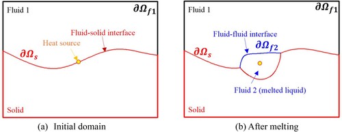
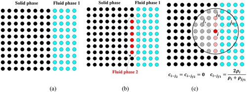
Initially, the computational domain contains a solid phase with a boundary of $\mathrm{\partial }{\mathrm{\Omega }}_s$ and a fluid phase with a boundary of $\mathrm{\partial }{\mathrm{\Omega }}_{f1}$, as displayed in Figure 1(a). The fluid phase is initially static and the liquid–solid interface is stable because there is no driving force for fluid motion at the initial moment. As indicated in Figure 1(a), a heat source is presented in the computational domain that transfers heat to the surrounding solid and liquid phases. The solid–liquid phase change occurs at the melting temperature and the solid phase turns into a liquid phase (i.e. Fluid 2 in Figure 1(b)). A solid phase with a boundary of $\mathrm{\partial }{\mathrm{\Omega }}_s$, a fluid phase with a boundary of $\mathrm{\partial }{\mathrm{\Omega }}_{f1}$, and a fluid phase with a boundary of $\mathrm{\partial }{\mathrm{\Omega }}_{f2}$ simultaneously exist in the domain. In the process of solid melting (i.e. Fluid 2), a new interface is formed between Fluid 1 and Fluid 2. The fluids start to move under the influence of gravity, viscosity, surface tension, and wetting effect. If the location and size of the heat source are time-dependent, fluid interfaces continue to appear and interact with the surrounding fluid, resulting in unstable and complex interface behavior.

Figure 1. Computational domain.

2.1.2 Unstable interface behavior caused by the phase change

As the solid–liquid phase change leads to the generation of new fluids, a new fluid interface is formed between the melted liquid (i.e. Fluid 2) and the ambient fluid (i.e. Fluid 1). The evolution process of the new fluid interface is governed by fluid dynamics, thermal dynamics, and is difficult to predict. Accurately calculating the evolution process of the interface is important for predicting the morphology of the metal after solidification and the heat-affected zone during the melting process (Cleary et al., 2006).

If there is a large density difference between Fluid 1 and Fluid 2 (for example, air and liquefied metal), the problem displayed in Figure 1(b) can be treated as a multiphase flow problem with a large density ratio. A stable simulation of this problem is a challenge for numerical methods; especially when there are unsteady interfaces and complex interface behavior, such as the generation of new interfaces (caused by melting), the disappearance of the old interface (caused by solidification), and fracture of the interface. Hence, to simulate such processes, efforts should be made to address the stability and accuracy problems caused by the solid–liquid phase transition and large density ratio.

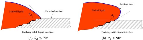
2.1.3 Wetting effect

As shown in Figure 2, a three-phase contact point is formed between the melted liquid (i.e. Fluid 2), the ambient fluid (i.e. Fluid 1), and the solid phase. At the triple contact point, the dynamic contact angle (see Figure 2, ${\theta }_d$) is used to describe the motion of fluid interface, which is affected by the wettability of the solid phase. In general, it is considered to be wetting when the contact angle is less than 90${}^{\circ }$ (see Figure 2(a)), and it is non-wetting when the contact angle is greater than 90${}^{\circ }$ (see Figure 2(b)). A proper description of the wetting effect is important for correctly simulating the fluid motion in the contact region. For the present problem, there are two challenges in modelling the wetting effect. First, the solid–liquid interface is constantly changing during the phase change, and the triple contact point, which is located at the melting front, is time-dependent. Second, the morphology of the evolving solid–liquid interface is transient and complex. A high effort could be associated with the determination of the dynamic contact angle.

Figure 2. Illustration of (a) wetting and (b) non-wetting effects of the solid surface by melted liquids.

2.2 Governing equations

2.2.1 Model for thermal dynamics

Considering the common forms of heat transfer in materials, the governing equation of thermal dynamics must cover the following processes: conduction, convection, source, and sink. In accordance with the Lagrangian nature of the SPH method, the adopted governing equation of thermal dynamics is expressed as the equation of the temperature rate: (1) $\rho c_p\frac{dT}{dt}=\mathrm{\nabla }\cdot \left(k\mathrm{\nabla }T\right)+{\dot{q}}_s^{\ast }+{\dot{q}}_l^{\ast },$(1) where $\rho$ is material density; T is temperature; k is the thermal conductivity; $c_p$ is the specific heat capacity. ${\dot{q}}_s^{\ast }$ and ${\dot{q}}_l^{\ast }$ denote the volumetric heat source and sink respectively. In Equation (1), the convection term is not explicitly given, as it is part of the substantial derivative on the left hand side. It is also noted that the volumetric heat source (as indicated in Figure 1) and sink are not considered in any of the examples simulated in this study. They are given in Equation (1) to ensure the completeness of the equation.

2.2.2 Model for solid–liquid phase change

The solid melting process is described by a phase change model (Farrokhpanah et al., 2017). In the model, the latent heat L absorbed/released from the melting/solidification of the material is determined by defining a transition zone around the melting temperature $T_m$. The transition zone is defined between $T_m-\mathrm{\Delta }T$ and $T_m+\mathrm{\Delta }T$ to prevent the phase transition point from being a mathematical singularity. The absorption of the latent heat is no longer a momentary process at the melting temperature. For the material experiencing a phase change, the equivalent heat capacity is assigned to the particle to substitute the actual heat capacity. The equivalent heat capacity is specified by the following equation: (2) $c_p=\{\begin{array}{ll}{c}_{ps}& T<T_m-\mathrm{\Delta }T\\ c_{pm}+{\displaystyle \frac{L}{2\mathrm{\Delta }T}}& T_m-\mathrm{\Delta }T\le T\le T_m+\mathrm{\Delta }T\\ c_{pl}& T>T_m+\mathrm{\Delta }T\end{array},$(2) where $c_{ps}$ and $c_{pl}$ denote the actual heat capacity of the solid and liquid phases, respectively, and $\mathrm{\Delta }T$ is the temperature interval of the transition zone. When the temperature of the material is located in transition zone, the equivalent heat capacity $c_{pm}+L/2\mathrm{\Delta }T$ is assigned to the material. In this phase change model, the temperature interval $\mathrm{\Delta }T$ should be carefully determined. The effect of latent heat could be bypassed if the temperature variation of an SPH particle during a time step exceeds $2\mathrm{\Delta }T$.

2.2.3 Model for fluid dynamics

The critical aspect of the SPH modeling of multiphase flows is to ensure the numerical stability of the interface, especially for the large-density-ratio problems. In the multiphase model of this study, the fluids on both sides of the interface are defined as the heavy and light phases, respectively. The governing equations of fluid dynamics including the continuity and momentum equations are expressed in the following Lagrangian form: (3) $\begin{array}{rl}\frac{D\rho }{Dt}& =-\rho \mathrm{\nabla }\cdot \mathit{v},\end{array}$(3) (4) $\begin{array}{rl}\frac{D\mathit{v}}{Dt}& =-\frac{1}{\rho }\mathrm{\nabla }p+\frac{\mu }{\rho }{\mathrm{\nabla }}^2\mathit{v}+{\mathit{F}}^B+{\mathit{F}}^S,\end{array}$(4) where ρ is the material density; $\mathit{v}$ is the velocity; t is the time; p is the pressure; $\mu$ is the dynamic viscosity. The solid melting process is assumed in the regime of laminar flow, which is modeled based on the Newton's law of viscosity. For further applications to the turbulent regime, a turbulent model should be adopted. ${\mathit{F}}^S$ and ${\mathit{F}}^B$ represent the surface tension and body force per unit mass.

In this study, the concerned fluid has a low velocity, corresponding to a small Mach number. Hence, both the gas and the liquid are considered as a incompressible fluid. In the SPH method, the incompressible fluid is usually treated as weakly–compressible. Hence, the continuity equation (Equation (3)) is written in the general case of a compressible fluid. In the weakly–compressible SPH, the density is allowed to vary, yet not exceed 1.0%, which is achieved by using a sufficiently large sound speed. Because the governing equations (i.e. Equations (3) and (4)) are not closed, the equation of state (EOS) is should be introduced to correlate the fluid pressure p and the density ρ. The EOS used in this study is expressed as (Batchelor, 1967): (5) $p=\frac{c^2{\rho }_0}{\gamma }\left({\left(\frac{\rho }{{\rho }_0}\right)}^{\gamma }-1\right)+p_b,$(5) where $\gamma$ is a constant and $p_b$ represents the background pressure. For a multicomponent domain containing two fluid phases, the EOS should be defined for each phase. Using the subscripts l and g represent the heavy and light phases, the EOS is expressed for the two phases as (Colagrossi & Landrini, 2003): (6) $\begin{array}{rl}{p}_l& =\frac{c_{0l}^2{\rho }_{0l}}{{\gamma }_l}\left({\left(\frac{{\rho }_l}{{\rho }_{0l}}\right)}^{{\gamma }_l}-1\right)+p_b,\end{array}$(6) (7) $\begin{array}{rl}{p}_g& =\frac{c_{0g}^2{\rho }_{0g}}{{\gamma }_g}\left({\left(\frac{{\rho }_g}{{\rho }_{0g}}\right)}^{{\gamma }_g}-1\right)+p_b,\end{array}$(7) where the parameter $\gamma$ is determined separately for the heavy and light phases, ${\gamma }_l=7$ and ${\gamma }_g=1.4$ (Colagrossi & Landrini, 2003); ${\rho }_{0l}$ and ${\rho }_{0g}$ represent the reference density of the heavy and light phases, respectively; $c_{0l}$ and $c_{0g}$ represent the reference sound speed of the heavy and light phases, respectively. The sound speed must be carefully selected to guarantee the weak compressibility of the fluid (< 1.0%). The fluid compressibility can be described using the Mach number: (8) $M{a}^2=\frac{v_b^2}{c^2}=\left|\frac{\rho -{\rho }_0}{{\rho }_0}\right|=\vartheta \rho ,$(8) where Ma represents the Mach number, v_b represents the characteristic velocity; $\vartheta$ is the relative change rate of the fluid density denoting the degree of compressibility of fluid. In this study, the sound speed of the heavy phase is determined first; then, the sound speed of the light phase is calculated based on their proportionality (see Equation (10)). Considering all the constraints related to inertial force, gravity, and surface tension, the sound speed of the heavy phase $c_l$ can be calibrated based on the following inequalities (Ming et al., 2017; Zhang et al., 2015): (9) $c_l\ge 10U_{max},c_l\ge 10\sqrt{g{L}_0},c_l\ge 10\sqrt{\frac{2\sigma }{{\rho }_{0l}R}},$(9) where $U_{max}$ represents the maximum velocity of the fluid; $R$ is the characteristic length or droplet radius; $g$ is the gravitational acceleration. The final value of the sound speed $c_l$ is the maximum of the calculations in Equation (9). Then, $c_g$ is calculated using the following equation (Colagrossi & Landrini, 2003; Zhang et al., 2015): (10) $c_g=\sqrt{c_l^2{\gamma }_g{\rho }_{0l}/\left({\gamma }_l{\rho }_{0g}\right)}.$(10)

The background pressure $p_b$ can prevent the net pressure of the fluid from being negative, which helps eliminate tension instability in SPH. In addition, the background pressure also helps to improve the stability of the interface with a large density ratio. Because the homogeneous background pressure is used for the entire fluid domain, it will not influence the flow field. However, an extremely low background pressure cannot effectively eliminate the negative pressure, whereas an extremely high background pressure can lead to excessive resetting of the particles. Hence, the value of $p_b$ should be carefully determined. In this study, the following equation is used to determine the value of background pressure (Ming et al., 2017): (11) $p_b=\alpha \frac{{\rho }_l-{\rho }_g}{{\rho }_l+{\rho }_g}\frac{\sigma }{R},$(11) where $\alpha$ is the coefficient and takes a value from 10 to 60 (Ming et al., 2017); $\sigma$ is the surface tension coefficient; $R$ is the droplet radius or the characteristic length. Equation (11) considers the effect of density difference. The greater the density difference (${\rho }_l-{\rho }_g$), the higher the corresponding background pressure value, which is more conducive to ensuring the stability of the interface (Ming et al., 2017).

2.3 Basic theory of SPH method

The computational domain of the SPH method is discretized by a finite number of particles (i.e. SPH particles) that carry an individual mass and occupy an individual space. The governing equations of continuum mechanics are then discretized based on these SPH particles. There are two key steps for the formulation using SPH. The first is the integral representation of the arbitrary field function. The idea of the integral representation of a function $f\left(\mathit{x}\right)$ comes from the following equation: (12) $f\left(\mathit{x}\right)=\int f\left({\mathit{x}}^{\mathbf{\prime }}\right)\delta \left(\mathit{x}-{\mathit{x}}^{\mathbf{\prime }}\right)d{\mathit{x}}^{\mathrm{\prime }},$(12) where $\delta \left(\mathit{x}-{\mathit{x}}^{\mathbf{\prime }}\right)$ is the Dirac delta function.

Using the kernel function to replace the Dirac delta function, the integral representation of $f\left(\mathit{x}\right)$ can be formulated as the kernel approximation (Liu & Liu, 2003): (13) $f\left(\mathit{x}\right)={\int }_{{\mathrm{\Omega }}_{\mathit{x}}}f\left({\mathit{x}}^{\mathbf{\prime }}\right)W\left(\mathit{x}-{\mathit{x}}^{\mathbf{\prime }},h\right)d{\mathit{x}}^{\mathrm{\prime }},$(13) where $f\left(\mathit{x}\right)$ is a field function related to the position vector $\mathit{x}$, $W\left(\mathit{x}-{\mathit{x}}^{\mathbf{\prime }},h\right)$ is the kernel function, and $h$ is the smoothing length. ${\mathrm{\Omega }}_{\mathit{x}}$ represents the integral volume containing $\mathit{x}$, and is also the so-called support domain. The kernel function is not unique, and it generally has the following properties: normalization, compact support, positivity, monotonicity, Delta function property, radial symmetry, and smoothness (Liu & Liu, 2003):

• (1) The kernel function must satisfy the normalization condition in the support domain: (14) ${\int }_{{\mathrm{\Omega }}_{\mathit{x}}}W\left(\mathit{x}-{\mathit{x}}^{\mathbf{\prime }},h\right)d{\mathit{x}}^{\mathbf{\prime }}=1.$(14)

• (2) The compact support condition defines the effective area of the kernel function as (15) $W\left(\mathit{x}-{\mathit{x}}^{\mathbf{\prime }},h\right)=0(\text{if }|\mathit{x}-{\mathit{x}}^{\mathbf{\prime }}|>ϵh),$(15) where $ϵ$ is the scale parameter and product $ϵh$ is equal to the radius of the support domain. Using this condition, integration over the entire computational domain can be localized over the support domain.

• (3) There is $W\left(\mathit{x}-{\mathit{x}}^{\mathbf{\prime }},h\right)\ge$0 (positivity) at any point ${\mathit{x}}^{\mathbf{\prime }}$ in the support domain of the point $\mathit{x}$.

• (4) When the distance between two points (i.e. $\mathit{x}$ and ${\mathit{x}}^{\mathbf{\prime }}$) increases, the value of the kernel function $W\left(\mathit{x}-{\mathit{x}}^{\mathbf{\prime }},h\right)$ should decrease monotonically (monotonicity).

• (5) When the smoothing length approaches 0, the kernel function should satisfy the Dirac function condition (Delta function property): (16) $\underset{h\to 0}{lim}W\left(\mathit{x}-{\mathit{x}}^{\mathbf{\prime }},h\right)=\delta \left(\mathit{x}-{\mathit{x}}^{\mathbf{\prime }}\right)\text{.}$(16)

• (6) The kernel function should be an even function (radial symmetry). This property means that points at the same distance from the given point but at different positions should have the same influence on the given point.

• (7) Kernel function should be sufficiently smooth (smoothness). Generally, the smoother the value of the kernel function, the better the result of the function and its derivative.

The approximate formula of the space derivative can be obtained using Equation (13), substituting $\left[\mathrm{\nabla }f\right]\left(\mathit{x}\right)$ for $f\left(\mathit{x}\right)$: (17) $\mathrm{\nabla }f\left(\mathit{x}\right)={\int }_{{\mathrm{\Omega }}_{\mathit{x}}}\left[\mathrm{\nabla }f\right]\left({\mathit{x}}^{\mathbf{\prime }}\right)W\left(\mathit{x}-{\mathit{x}}^{\mathbf{\prime }},h\right)d{\mathit{x}}^{\mathrm{\prime }}.$(17) Since (18) $\begin{array}{rl}\left[\mathrm{\nabla }f\right]\left({\mathit{x}}^{\mathbf{\prime }}\right)W\left(\mathit{x}-{\mathit{x}}^{\mathbf{\prime }},h\right)& =\mathrm{\nabla }\left[f\left({\mathit{x}}^{\mathbf{\prime }}\right)W\left(\mathit{x}-{\mathit{x}}^{\mathbf{\prime }},h\right)\right]\\ & -f\left({\mathit{x}}^{\mathbf{\prime }}\right){\mathrm{\nabla }}_{{\mathit{x}}^{\mathbf{\prime }}}W\left(\mathit{x}-{\mathit{x}}^{\mathbf{\prime }},h\right).\end{array}$(18)

From Equation (17), the following equation is obtained, (19) $\begin{array}{rl}\mathrm{\nabla }f\left(\mathit{x}\right)& ={\int }_{{\mathrm{\Omega }}_{\mathit{x}}}\mathrm{\nabla }\left[f\left({\mathit{x}}^{\mathbf{\prime }}\right)W\left(\mathit{x}-{\mathit{x}}^{\mathbf{\prime }},h\right)\right]d{\mathit{x}}^{\mathrm{\prime }}\\ & -{\int }_{{\mathrm{\Omega }}_{\mathit{x}}}f\left({\mathit{x}}^{\mathbf{\prime }}\right){\mathrm{\nabla }}_{{\mathit{x}}^{\mathbf{\prime }}}W\left(\mathit{x}-{\mathit{x}}^{\mathbf{\prime }},h\right)d{\mathit{x}}^{\mathrm{\prime }}.\end{array}$(19) The first term on the right side of Equation (19) can be applied to the Gauss theorem to transform the integral on the volume ${\mathrm{\Omega }}_{\mathit{x}}$ into the integral on the surface S. After the transformation, the following equation is obtained: (20) $\begin{array}{rl}\mathrm{\nabla }f\left(\mathit{x}\right)& ={\int }_{S}f\left(x^{\mathrm{\prime }}\right)W\left(\mathit{x}-{\mathit{x}}^{\mathbf{\prime }},h\right)\mathit{n}dS\\ & -{\int }_{{\mathrm{\Omega }}_{\mathit{x}}}f\left({\mathit{x}}^{\mathbf{\prime }}\right){\mathrm{\nabla }}_{{\mathit{x}}^{\mathbf{\prime }}}W\left(\mathit{x}-{\mathit{x}}^{\mathbf{\prime }},h\right)d{\mathit{x}}^{\mathrm{\prime }},\end{array}$(20) where $\mathit{n}$ is the unit normal vector of the boundary of the support domain. According to the compact support condition (Equation (15)), the surface integral on the right side of the Equation (20) vanishes. Hence, the approximation of the gradient of a scalar function $f\left(\mathit{x}\right)$ is: (21) $\mathrm{\nabla }f\left(\mathit{x}\right)=-{\int }_{{\mathrm{\Omega }}_{\mathit{x}}}f\left({\mathit{x}}^{\mathbf{\prime }}\right){\mathrm{\nabla }}_{{\mathit{x}}^{\mathbf{\prime }}}W\left(\mathit{x}-{\mathit{x}}^{\mathbf{\prime }},h\right)d{\mathit{x}}^{\mathrm{\prime }}.$(21) Similarly, the approximation of the divergent of a vectorial function $\mathit{f}\left(\mathit{x}\right)$ can be obtained: (22) $\mathrm{\nabla }\cdot \mathit{f}\left(\mathit{x}\right)=-{\int }_{{\mathrm{\Omega }}_{\mathit{x}}}\mathit{f}\left({\mathit{x}}^{\mathbf{\prime }}\right)\cdot {\mathrm{\nabla }}_{{\mathit{x}}^{\mathbf{\prime }}}W\left(\mathit{x}-{\mathit{x}}^{\mathbf{\prime }},h\right)d{\mathit{x}}^{\mathrm{\prime }}.$(22)

Since the kernel function satisfies the symmetry condition, the following relation exists: $\begin{array}{rl}{\mathrm{\nabla }}_{{\mathit{x}}^{\mathbf{\prime }}}W\left(\mathit{x}-{\mathit{x}}^{\mathbf{\prime }},h\right)d{\mathit{x}}^{\mathbf{\prime }}& =\frac{\mathrm{\partial }W\left(\mathit{x}-{\mathit{x}}^{\mathbf{\prime }},h\right)}{\mathrm{\partial }{\mathit{x}}^{\mathbf{\prime }}}\\ & =-\frac{\mathrm{\partial }W\left(\mathit{x}-{\mathit{x}}^{\mathbf{\prime }},h\right)}{\mathrm{\partial }\mathit{x}}\\ & =-{\mathrm{\nabla }}_{\mathit{x}}W\left(\mathit{x}-{\mathit{x}}^{\mathbf{\prime }},h\right)d{\mathit{x}}^{\mathrm{\prime }}.\end{array}$ Then, Equations (21) and (22) can be written as: (23) $\begin{array}{rl}\mathrm{\nabla }f\left(\mathit{x}\right)& ={\int }_{{\mathrm{\Omega }}_{\mathit{x}}}f\left({\mathit{x}}^{\mathbf{\prime }}\right){\mathrm{\nabla }}_{\mathit{x}}W\left(\mathit{x}-{\mathit{x}}^{\mathbf{\prime }},h\right)d{\mathit{x}}^{\mathrm{\prime }},\end{array}$(23) (24) $\begin{array}{rl}\mathrm{\nabla }\cdot \mathit{f}\left(\mathit{x}\right)& ={\int }_{{\mathrm{\Omega }}_{\mathit{x}}}\mathit{f}\left({\mathit{x}}^{\mathbf{\prime }}\right)\cdot {\mathrm{\nabla }}_{\mathit{x}}W\left(\mathit{x}-{\mathit{x}}^{\mathbf{\prime }},h\right)d{\mathit{x}}^{\mathrm{\prime }}.\end{array}$(24) As the computational domain is discretized with particles (see Figure 3), the field function at a particle (i.e. i) can be obtained simply through summations over all particles within the support domain of the particle (${\mathrm{\Omega }}_{{\mathit{x}}_{\mathit{i}}}$) using a kernel function. This step is the so-called particle approximation. According to Equations (13) and (23), the particle approximation for a function and its spatial derivatives at particle i can be expressed as (Liu & Liu, 2003): (25) $\begin{array}{rl}f\left({\mathit{x}}_i\right)& =\sum _{j=1}^{N_i}\frac{m_j}{{\rho }_j}f\left({\mathit{x}}_j\right)W\left({\mathit{x}}_i-{\mathit{x}}_j,h\right),\end{array}$(25) (26) $\begin{array}{rl}\mathrm{\nabla }f\left({\mathit{x}}_i\right)& =\sum _{j=1}^{N_i}\frac{m_j}{{\rho }_j}f\left({\mathit{x}}_j\right){\mathrm{\nabla }}_{{\mathit{x}}_i}\text{W}\left({\mathit{x}}_i-{\mathit{x}}_j,h\right),\end{array}$(26) where j represents the particle located in the support domain of particle i and ${\mathrm{\nabla }}_{{\mathit{x}}_i}\text{W}\left({\mathit{x}}_i-{\mathit{x}}_j,h\right)$ is the gradient of the kernel with respect to particle i; ρ_j is the density of the particle j; m_j is the mass of the particle j.

Figure 3. Particle distribution within the support domain of the smoothing function W for particle i. The support domain (${\mathrm{\Omega }}_{{\mathit{x}}_{\mathit{i}}}$) and its boundary S is circular with the radius of $ϵh$. The figure is cited from the book by Liu & Liu, 2003.

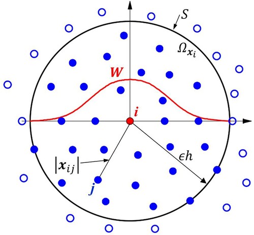
In SPH, there are many choices for the kernel function $W$. Jing and Ding (Jing & Ding, 2005) conducted a comparative study on more than ten kernel functions, and concluded that the 5th-order spline and the Gaussian functions give better results in terms of accuracy and stability. The two kernel functions have a relatively large cut-off radius (3h) and have more particles in the support domain. In this study, the Gaussian function is adopted as the kernel function which is expressed as follows (Grenier et al., 2009; Molteni & Colagrossi, 2009): (27) $W\left(r,h\right)=\frac{1}{\pi h^2}\{\begin{array}{ll}{\displaystyle \frac{e^{-{\left(r/h\right)}^2}-C_0}{1-C_1}},& r\le 3h\\ 0,& r>3h\end{array},$(27) where h represents the smoothing length, and r = $|\mathit{x}-{\mathit{x}}^{\mathbf{\prime }}|$. The constants $C_0$ and $C_1$ are introduced to obtain a Gaussian kernel function with a compact support, and they are set as $C_0=e^{-9}$ and $C_1=10C_0$. In this study, the smoothing length is chosen as 1.33 times the particle spacing (i.e. $h=1.33\mathrm{\Delta }x$, $\mathrm{\Delta }x$ is the initial particle spacing), and the support domain radius is 3.99$\mathrm{\Delta }x$.

3. Numerical model based on SPH

3.1 Discrete form of governing equation of thermal dynamics

The discrete form of the governing equation of thermal dynamics (Equation (1)) without the heat source and sink terms is expressed as (Cleary & Monaghan, 1999): (28) $\begin{array}{rl}{c}_{p,i}\frac{d{T}_i}{dt}& =\sum _{j=1}^{N_i}\frac{m_j}{{\rho }_i{\rho }_j}\left(k_i+k_j\right)\left(T_i-T_j\right)\\ & \times \frac{{\mathit{x}}_{ij}\cdot {\mathrm{\nabla }}_{{\mathit{x}}_i}\text{W}\left({\mathit{x}}_i-{\mathit{x}}_j,h\right)}{{\mathit{x}}_{ij}^2},\end{array}$(28) where ${\mathit{x}}_{ij}$ = ${\mathit{x}}_i-{\mathit{x}}_j$, $k_i$ and $k_j$ represent the thermal conductivity of particles i and j. Because of the radially symmetric property of the kernel, the kernel gradient ${\mathrm{\nabla }}_{{\mathit{x}}_i}\text{W}\left({\mathit{x}}_i-{\mathit{x}}_j,h\right)$ can be written as $\frac{{\mathit{x}}_{ij}}{|{\mathit{x}}_{ij}|}\frac{\mathrm{\partial }W\left({\mathit{x}}_i-{\mathit{x}}_j,h\right)}{\mathrm{\partial }|{\mathit{x}}_i-{\mathit{x}}_j|}$. Hence, the notation $\frac{{\mathit{x}}_{ij}\cdot {\mathrm{\nabla }}_{{\mathit{x}}_i}\text{W}\left({\mathit{x}}_i-{\mathit{x}}_j,h\right)}{{\mathit{x}}_{ij}^2}$ in Equation (28) simplifies to $\frac{1}{|{\mathit{x}}_{ij}|}\frac{\mathrm{\partial }W\left({\mathit{x}}_i-{\mathit{x}}_j,h\right)}{\mathrm{\partial }|{\mathit{x}}_i-{\mathit{x}}_j|}$. Equation (28) is transformed into: (29) $\begin{array}{rl}{c}_{p,i}\frac{d{T}_i}{dt}& =\sum _{j=1}^{N_i}\frac{m_j}{{\rho }_i{\rho }_j}\left(k_i+k_j\right)\left(T_i-T_j\right)\frac{1}{|{\mathit{x}}_{ij}|}\\ & \times \frac{\mathrm{\partial }W\left({\mathit{x}}_i-{\mathit{x}}_j,h\right)}{\mathrm{\partial }|{\mathit{x}}_i-{\mathit{x}}_j|}.\end{array}$(29)

However, Equation (29) does not guarantee the continuous distribution of the heat flux across the interface. Cleary and Monaghan (1999) solved this problem by replacing $\left(k_i+k_j\right)$ by $4k_i{k}_j/\left(k_i+k_j\right)$. The use of $4k_i{k}_j/\left(k_i+k_j\right)$ at the interface is more conducive to obtaining continuous heat flux than that of $\left(k_i+k_j\right)$, even if the ratio of thermal conductivity (i.e. $k_i/k_j$ or $k_j/k_i$) on both sides of the interface reaches 10³ (Cleary & Monaghan, 1999; Monaghan et al., 2005). Hence, the finally adopted discrete equation of thermal dynamics is expressed as: (30) $c_{p,i}\frac{d{T}_i}{dt}=\sum _{j=1}^{N_i}\frac{4m_j}{{\rho }_i{\rho }_j}\frac{k_i{k}_j}{k_i+k_j}\left(T_i-T_j\right)\frac{1}{|{\mathit{x}}_{ij}|}\frac{\mathrm{\partial }W\left({\mathit{x}}_i-{\mathit{x}}_j,h\right)}{\mathrm{\partial }|{\mathit{x}}_i-{\mathit{x}}_j|}.$(30)

3.2 SPH model for multiphase flow

3.2.1 SPH discrete equations

As the governing equations (Equations (3) and (4)) are expressed in Lagrangian form, the discrete governing equations are expressed in the form of the derivative of density (for the continuity equation) and the derivative of velocity (for the momentum equation) of the particle. The pressure gradient and viscous force terms on the right-hand side (RHS) of Equation (4) are transformed into the summation form of SPH particles. The pressure gradient term usually employs the anti–symmetric discrete gradient operator (31) $\begin{array}{rl}-\frac{1}{{\rho }_i}{\mathit{G}}_i^{+}\left(p_j\right)& =-\sum _{j=1}^{N_i}{m}_j\left(\frac{p_i}{{\rho }_i^2}+\frac{p_j}{{\rho }_j^2}\right){\mathrm{\nabla }}_{{\mathit{x}}_i}W\left({\mathit{x}}_i-{\mathit{x}}_j,h\right)\\ & \approx -{\left(\frac{1}{\rho }\mathrm{\nabla }p\right)}_i.\end{array}$(31) The particle approximation of the divergence of velocity vector is usually expressed as: (32) $\begin{array}{rl}{D}_i^{-}\left({\mathit{v}}_j\right)& =\frac{1}{{\rho }_i}\sum _{j=1}^{N_i}{m}_j\left({\mathit{v}}_j-{\mathit{v}}_i\right)\cdot {\mathrm{\nabla }}_{{\mathit{x}}_i}W\left({\mathit{x}}_i-{\mathit{x}}_j,h\right)\\ & \approx (\mathrm{\nabla }\cdot \mathit{v}{)}_i.\end{array}$(32)

Based on Equations (31) and (32), the discrete form of governing equations can be expressed as follows: (33) $\begin{array}{rl}\frac{d{\rho }_i}{dt}& =\sum _{j=1}^{N_i}{m}_j\left({\mathit{v}}_i-{\mathit{v}}_j\right)\cdot {\mathrm{\nabla }}_{{\mathit{x}}_i}W\left({\mathit{x}}_i-{\mathit{x}}_j,h\right),\end{array}$(33) (34) $\begin{array}{rl}\frac{d{\mathit{v}}_i}{dt}& =-\sum _{j=1}^{N_i}{m}_j\left(\frac{p_i}{{\rho }_i^2}+\frac{p_j}{{\rho }_j^2}\right){\mathrm{\nabla }}_{{\mathit{x}}_i}W\left({\mathit{x}}_i-{\mathit{x}}_j,h\right)\\ & +{\left(\frac{\mu }{\rho }{\mathrm{\nabla }}^2\mathit{v}\right)}_i+{\mathit{F}}_i^B+{\mathit{F}}_i^S,\end{array}$(34) where ${\rho }_i$, ${\rho }_j$,$m_i$, and $m_j$ represent the density and mass of the particles i and j, respectively. $N_i$ represents the number of neighboring particles. However, Equations (33) and (34) cannot be directly applied to multiphase flow simulations. For the large-density-ratio problem, the sudden change in density and mass across the interface could result in numerical discontinuities. Hence, Colagrossi and Landrini (2003) suggested a modified version of the continuity equation for multiphase simulations, (35) $\frac{d{\rho }_i}{dt}={\rho }_i\sum _{j=1}^{N_i}\frac{m_j}{{\rho }_j}\left({\mathit{v}}_i-{\mathit{v}}_j\right)\cdot {\mathrm{\nabla }}_{{\mathit{x}}_i}W\left({\mathit{x}}_i-{\mathit{x}}_j,h\right).$(35) Equation (35) is obtained by replacing $m_j$ in Equation (33) with $\frac{{\rho }_i{m}_j}{{\rho }_j}$, where $\frac{m_j}{{\rho }_j}$ corresponds to the volume of the particle j. This form of continuity equation has been used in many previous models for various applications, such as bubble dynamics, underwater explosions (Colagrossi & Landrini, 2003; Liu et al., 2003; Zhang et al., 2012).

Hu and Adams (2006) proposed another density scheme for multiphase simulations. To solve the problem of the discontinuity of particle density and mass at the interface, the particle–approximated equation based on particle volume is derived (Hu & Adams, 2006). In this scheme, the particle volume is first calculated based on the current particle distribution using kernel summation: (36) $V_i=\frac{1}{{\sum }_{j=1}^{N_i}\text{W}\left({\mathit{x}}_i-{\mathit{x}}_j,h\right)}.$(36) Equation 36 takes into account the fact that: (37) $\frac{1}{V_i}=\sum _{j=1}^{N_i}\frac{1}{V_j}\text{W}\left({\mathit{x}}_i-{\mathit{x}}_j,h\right)V_j=\sum _{j=1}^{N_i}\text{W}\left({\mathit{x}}_i-{\mathit{x}}_j,h\right).$(37)

In consideration of the conservation of particle mass $m_i$, the density of the particle can be calculated by: (38) ${\rho }_i=\frac{m_i}{V_i},{\rho }_i=m_i\sum _{j=1}^{N_i}\text{W}\left({\mathit{x}}_i-{\mathit{x}}_j,h\right).$(38) where $V_i$ represents the volume of the particle i; ρ_i is the density of particle i; m_i is the mass of the particle. In this study, computational domains for different phases use the same initial particle spacing and particle volume. Because of the weakly compressible condition, the particle volume changes insignificantly during the simulation. There is no sudden change in particle volume across the interface, even for the large-density-ratio problem. Therefore, the volume-based density approximation scheme has better adaptability to the large-density-ratio problem.

Similarly, for the approximation of pressure gradient term, the volume-based scheme is also used. Assuming that $V_i=V_j$, the discrete form of the pressure gradient term can be written as (Hu & Adams, 2006; Zhang et al., 2012): (39) $\begin{array}{rl}-{\left(\frac{1}{\rho }\mathrm{\nabla }p\right)}_{\text{i}}& \approx -\frac{1}{{\rho }_i{V}_i}\sum _{j=1}^{N_i}\left(p_i{V}_i^2+p_j{V}_j^2\right)\\ & \times {\mathrm{\nabla }}_{{\mathit{x}}_i}\text{W}\left({\mathit{x}}_i-{\mathit{x}}_j,h\right),\end{array}$(39) where $p_i$, $V_i$, $p_j$, and $V_j$ denote the pressure and volume of particles i and j, respectively.

There are two commonly used discrete forms of the viscous term in SPH. The first one was proposed by Monaghan and Gingold (1983) and refers to Type 1 in this study. The second was originally proposed by Morris et al. (1997), modified by Hu and Adams (2006), and tested by Grenier et al. (Grenier et al., 2013), predicting more accurate results than the first. The two types of the viscous term are expressed as: (40) $\begin{array}{rl}\text{Type }1:(\mu {\mathrm{\nabla }}^2\mathit{v}{)}_i& =\sum _j^{N_i}8{\mu }_{ij}{V}_j\frac{\left({\mathit{v}}_i-{\mathit{v}}_{\mathit{j}}\right)\cdot \left({\mathit{x}}_i-{\mathit{x}}_{\mathit{j}}\right)}{{|{\mathit{x}}_i-{\mathit{x}}_{\mathit{j}}|}^2+{\left(0.01h\right)}^2}\\ & \times {\mathrm{\nabla }}_{{\mathit{x}}_i}\text{W}\left({\mathit{x}}_i-{\mathit{x}}_j,h\right),\end{array}$(40) (41) $\begin{array}{rl}\text{Type }2:(\mu {\mathrm{\nabla }}^2\mathit{v}{)}_i& =\sum _j^{N_i}{\mu }_{ij}\frac{\left(V_i^2+V_j^2\right)}{V_i}\frac{1}{|{\mathit{x}}_{ij}|}\\ & \times \frac{\mathrm{\partial }W\left({\mathit{x}}_i-{\mathit{x}}_j,h\right)}{\mathrm{\partial }|{\mathit{x}}_i-{\mathit{x}}_j|}\left({\mathit{v}}_i-{\mathit{v}}_{\mathit{j}}\right),\end{array}$(41) where the parameter ${\mu }_{ij}=\frac{2{\mu }_i{\mu }_j}{{\mu }_i+{\mu }_j}$, ${\mu }_i$ and ${\mu }_{\text{j}}$ represent the dynamic viscosity of particles i and j, respectively. In this study, the second one (i.e. Type 2) is adopted.

3.2.2 Surface tension modeling

Based on the continuum surface force (CSF) method, the surface tension force is expressed as follows (Brackbill et al., 1992): (42) ${\mathit{F}}^S=-\frac{\sigma \xi \mathit{n}\lambda }{\rho },$(42) where $\sigma$ represents the surface tension coefficient; ξ represents the curvature, n is the normal vector, and λ is the weight function which ensures that the force is applied only to the fluid located at the interface. The color function is defined to calculate the normal vector of the interface (Morris, 2000), (43) $c_i^j=\{\begin{array}{ll}1& \begin{array}{l}\text{if particles }i\text{ and }j\\ \text{ belong to different phases}\end{array}\\ 0& \begin{array}{l}\text{if particles }i\text{ and }j\\ \text{ belong to same phase}\end{array}\end{array}.$(43)

Equation (43) does not consider the change in density and mass across the interface; hence, an density-weighted form of the color function is used in this study (Adami et al., 2010; Zhang et al., 2015): (44) $c_i^j=\{\begin{array}{ll}{\displaystyle \frac{2{\rho }_i}{{\rho }_i+{\rho }_j}}& \begin{array}{l}\text{if particles }i\text{ and }j\\ \text{ belong to different phases}\end{array}\\ 0& \begin{array}{l}\text{if particles }i\text{ and }j\\ \text{ belong to same phase}\end{array}\end{array}.$(44) By calculating the gradient of color function, the normal vector of particle i at the interface can be calculated as: (45) ${\mathit{n}}_{\mathit{i}}=\frac{\mathrm{\nabla }{c}_i}{|\mathrm{\nabla }{c}_i|},$(45) where ${\mathit{n}}_{\mathit{i}}$ is the unit normal vector of particle i at the interface and $\mathrm{\nabla }{c}_i$ is the gradient of color function, which is calculated by (Adami et al., 2010; Zhang et al., 2015): (46) $\mathrm{\nabla }{c}_i=\frac{1}{V_i}\sum _{j=1}^{N_i}\left(V_i^2+V_j^2\right)\frac{c_i^i+c_i^j}{2}{\mathrm{\nabla }}_{{\mathit{x}}_i}W\left({\mathit{x}}_i-{\mathit{x}}_j,h\right),$(46) where $c_i^i$ and $c_i^j$ can be calculated using Equation (44). In addition, $|\mathrm{\nabla }{c}_i|$ has the role of the Dirac function, which can ensure the continuity of particle acceleration across the interface. To calculate the curvature of the interface, another color function is introduced (Zhang et al., 2015): (47) ${\phi }_i^j=\{\begin{array}{ll}-1& \begin{array}{l}\text{if particles }i\text{ and }j\\ \text{ belong to different phases}\end{array}\\ 1& \begin{array}{l}\text{if particles }i\text{ and }j\\ \text{ belong to same phase}\end{array}\end{array}.$(47)

Then the curvature of interface particle i can be calculated by (Zhang et al., 2015): (48) ${\xi }_i=-\mathrm{\nabla }\cdot {\mathit{n}}_{\mathit{i}}=-d\frac{{\sum }_{j=1}^{N_i}\left({\mathit{n}}_{\mathit{i}}-{\phi }_i^j{\mathit{n}}_{\mathit{j}}\right){\mathrm{\nabla }}_{{\mathit{x}}_i}W\left({\mathit{x}}_i-{\mathit{x}}_j,h\right)V_j}{{\sum }_{j=1}^{N_i}|{\mathit{x}}_i-{\mathit{x}}_j||{\mathrm{\nabla }}_{{\mathit{x}}_i}\text{W}\left({\mathit{x}}_i-{\mathit{x}}_j,h\right)|V_j},$(48) where d represents the dimension of space (for 2D problems, d = 2), and the value of the color function ${\phi }_i^j$ is calculated by Equation (47). In Equation (48), the color function ${\phi }_i^j$ is used to point the normal vector of the fluid particles at the interface to the other side of the interface.

Substituting Equations (45) (46) and (48) into Equation (42), the surface tension force ${\mathit{F}}_i^S$ of particle i can be expressed as follows: (49) $\begin{array}{rl}{\mathit{F}}_i^S& =-\frac{\sigma {\xi }_i{\mathit{n}}_{\mathit{i}}\mathrm{\nabla }{c}_i}{{\rho }_i}\\ & =\frac{\begin{array}{c}\sigma \left(\sum _{j=1}^{N_i}\left({\mathit{n}}_{\mathit{i}}-{\phi }_i^j{\mathit{n}}_{\mathit{j}}\right){\mathrm{\nabla }}_{{\mathit{x}}_i}W\left({\mathit{x}}_i-{\mathit{x}}_j,h\right)V_j\right)\\ \left(\sum _{j=1}^{N_i}\left(V_i^2+V_j^2\right)\left(c_i^i+c_i^j\right){\mathrm{\nabla }}_{{\mathit{x}}_i}W\left({\mathit{x}}_i-{\mathit{x}}_j,h\right)\right)\end{array}}{\begin{array}{c}{\rho }_i{V}_i\sum _{j=1}^{N_i}|{\mathit{x}}_i-{\mathit{x}}_j|\\ |{\mathrm{\nabla }}_{{\mathit{x}}_i}\text{W}\left({\mathit{x}}_i-{\mathit{x}}_j,h\right)|V_j\end{array}}\end{array}$(49)

3.2.3 Treatment of the interface

In the interactive region between two phases, as indicated in Figure 4, the location of the interface can be identified from the particle distribution of the two phases (Fluid 1 and Fluid 2 in Figure 4(a)). In the case of a large density ratio, particles near the interface could be distributed in a disorderly fashion (Figure 4(b)), and particles of the two phases tend to penetrate each other. Hence, techniques must be used to prevent the particles from penetrating the interface.

Figure 4. Illustration of particles near the interface.

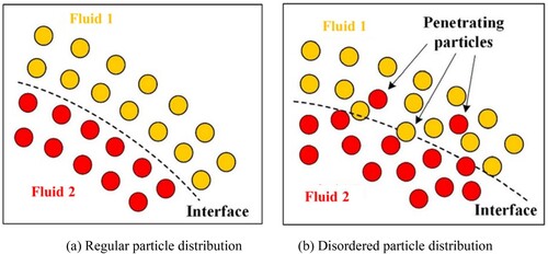
In this study, the interface sharpness force (ISF) which was initially proposed by Grenier et al. (2009), and modified by Zhang et al. (2015), is adopted. The interface sharpness force is expressed as: (50) ${\mathit{F}}_{\text{i}}^{interface}=\frac{\zeta }{{\rho }_{\text{i}}{V}_i}\sum _{j=1}^{N_i}\left(|{p_i}_{}|V_i^2+|p_j|V_j^2\right){\mathrm{\nabla }}_{{\mathit{x}}_i}W\left({\mathit{x}}_i-{\mathit{x}}_j,h\right),$(50) where $\zeta$ is a constant, typically taking the value of 0.08 (Zhang et al., 2015). Moreover, to obtain uniform particle distributions, a particle shifting algorithm (Xu et al., 2009) is used to correct the position of particles during the simulation.

The interface sharpness force (Equation (50)) is only used for the interface particles between different fluid phases. It helps to maintain the stability at the interface between the new melted liquid (i.e. Fluid 2) and the original (ambient) fluid (i.e. Fluid 1). In this study, the computational domain contains at least three phases. The interface sharpness force is activated in two situations: (a) between Fluid 1 and Fluid 2, and (b) between Fluid 1 and the solid phase. As displayed in Figure 5, Fluid 1 and the solid phase are considered as the same phase. In this case, the surface tension always causes the contact angle of the melted liquid (Fluid 2) and solid surface to be zero. Therefore, the treatment shown in Figure 5 is suitable for the situation that the solid surface can be wetted by the molten liquid. In the Section 3.2.4, the modeling of wetting/non-wetting effects of solid surface by melted liquids is introduced in detail.

Figure 5. Treatment for new interface particles for considering the wetting effect.

It is noted that both the solid and fluid domains are discretized into SPH particles using the same initial particle spacing $\mathrm{\Delta }x$. For solid particles, only the thermal dynamics model is used, and the position of the solid particle is fixed . For fluid particles, both the thermal dynamics and fluid dynamics model are used. For solid particles close to the solid–liquid interface, to calculate the force of the solid particles on the fluid particles, the pressure of the solid particles is also calculated by the EOS, thus the solid particles are involved in the kernel approximation of the fluid particles.

3.2.4 Wetting effect modeling

As discussed in Section 2.1.3, a proper description of the wettability of the solid surface is important for simulating the interface behavior of the melting flow. Figure 5 displays the treatment method for the wetting of the solid surface by melted liquids. Similarly, for the case of non–wetting of the solid surface, the solid phase and Fluid 1 are regarded as one phase when calculating the surface tension. The above treatment provides a simple way to simulate wetting and non–wetting effects of the solid surface. However, for characterizing the wettability of the solid surface quantitatively, the contact angle model is required.

Researchers have proposed many methods for modeling the wetting effect and contact angle in SPH. They can be divided into two categories. The first category simulates the contact angle by correcting the normal vector at the contact line (Breinlinger et al., 2013) or by establishing a virtual interface to adjust the contact line geometrically (Dong et al., 2019; Yeganehdoust et al., 2016). The second category simulates the wetting effect using an inter–phase force model which is analogous to the inter–molecular force (Tartakovsky & Meakin, 2005). In the first category, the contact angle is considered as an input parameter, and it can be combined with the CSF method. However, it requires a fixed liquid–solid interface, hence it is not suitable for the melting flow that the solid boundary evolves.

From a mechanical point of view, the wetting phenomenon is caused by the interaction among different phases at the triple contact region. In this study, the triple contact region containing solid phase, Fluid 1 and Fluid 2. We adopts the method similar to that in the literature (Hu & Adams, 2006; Ming et al., 2017) for simulating wetting/no-wetting effects. For a particle i from Fluid 2, if there are a solid phase and Fluid 1 in its support domain, the gradient of the color function $\mathrm{\nabla }{c}_i$ can be decomposed into two parts, $\mathrm{\nabla }{c}_i^{f_2-s}$ and $\mathrm{\nabla }{c}_i^{f_2-f_1}$, and are calculated separately: (51) $\{\begin{array}{l}\mathrm{\nabla }{c}_i^{f_2-s}={\displaystyle \frac{1}{V_i}}\sum _{j=1}^{N_i}\left(V_i^2+V_j^2\right){\displaystyle \frac{c_i^i+c_i^j}{2}}\\ {\mathrm{\nabla }}_{{\mathit{x}}_i}W\left({\mathit{x}}_i-{\mathit{x}}_j,h\right)ifj\in {\mathrm{\Omega }}_{f2}\cup {\mathrm{\Omega }}_s\\ \mathrm{\nabla }{c}_i^{f_2-f_1}={\displaystyle \frac{1}{V_i}}\sum _{j=1}^{N_i}\left(V_i^2+V_j^2\right){\displaystyle \frac{c_i^i+c_i^j}{2}}\\ {\mathrm{\nabla }}_{{\mathit{x}}_i}W\left({\mathit{x}}_i-{\mathit{x}}_j,h\right)ifj\in {\mathrm{\Omega }}_{f2}\cup {\mathrm{\Omega }}_{f1}\end{array}$(51) where $\mathrm{\nabla }{c}_i^{f_2-s}$ and $\mathrm{\nabla }{c}_i^{f_2-f_1}$ represent the gradient of color function calculated between Fluid 2 and solid, and between Fluid 1 and Fluid 2, respectively.

Similarly, components of unit normal vector are also calculated separately: (52) $\{\begin{array}{l}{\mathit{n}}_{\mathit{i}}^{f_2-s}={\displaystyle \frac{\mathrm{\nabla }{c}_i^{f_2-s}}{|\mathrm{\nabla }{c}_i^{f_2-s}|}}\\ {\mathit{n}}_{\mathit{i}}^{f_2-f_1}={\displaystyle \frac{\mathrm{\nabla }{c}_i^{f_2-f_1}}{|\mathrm{\nabla }{c}_i^{f_2-f_1}|}}\end{array},$(52) and the surface tensions on the solid–fluid interface and fluid–fluid interface are calculated by (53) $\{\begin{array}{l}{\mathit{F}}_i^{f_2-s}=-{\sigma }^{f_2-s}{\xi }_i^{f_2-s}{\mathit{n}}_{\mathit{i}}^{f_2-s}|\mathrm{\nabla }{c}_i^{f_2-s}|\\ {\mathit{F}}_i^{f_2-f_1}=-{\sigma }^{f_2-f_1}{\xi }_i^{f_2-f_1}{\mathit{n}}_{\mathit{i}}^{f_2-f_1}|\mathrm{\nabla }{c}_i^{f_2-f_1}|\end{array}.$(53) where ${\sigma }^{f_2-s}$ and ${\sigma }^{f_2-f_1}$ are the surface tension coefficients between Fluid 2 and solid, and between Fluid 1 and Fluid 2, respectively.

Then, the surface tension force of the particle i in the triple contact region can be expressed as: (54) ${\mathit{F}}_i^S={\mathit{F}}_i^{f_2-s}+{\mathit{F}}_i^{f_2-f_1}.$(54)

3.3 Time integration scheme

An efficient time integration scheme proposed by Zhang et al. (2015) is adopted in this study. As described by Zhang et al. (2015), this scheme is the combination of the velocity-Verlet scheme (Adami et al., 2012; Verlet, 1967) and the prediction-correction time step scheme (Chen et al., 2015; Monaghan, 1989). Because it is similar to the modified Verlet scheme applied in Molteni and Colagrossi (Molteni & Colagrossi, 2009), a larger Courant–Friedrichs–Lewy (CFL) factor can be used (Zhang et al., 2015). In this scheme, field variables are updated twice in a single time step (i.e. from n to n+1). Hence, it is like a mid-point linear two-step scheme.

At the time step of n, the derivatives ${\left(\frac{d\mathit{v}}{dt}\right)}_i$ and ${\left(\frac{dT}{dt}\right)}_i$ are first calculated. Then, the velocity ${\mathit{v}}_{\text{i}}^{\text{n}+1/2}$, position ${\mathit{x}}_{\text{i}}^{\text{n}+1/2}$, and temperature $T_i^{n+1/2}$ are updated by the following equations: (55) $\{\begin{array}{l}{\mathit{v}}_i^{n+1/2}={\mathit{v}}_i^n+{\left({\displaystyle \frac{d\mathit{v}}{dt}}\right)}_i^n{\displaystyle \frac{\mathrm{\Delta }t}{2}}\\ {\mathit{x}}_i^{n+1/2}={\mathit{x}}_i^n+{\mathit{v}}_i^{n+1/2}{\displaystyle \frac{\mathrm{\Delta }t}{2}}\\ T_i^{n+1/2}=T_i^n+{\left({\displaystyle \frac{dT}{dt}}\right)}_i^n{\displaystyle \frac{\mathrm{\Delta }t}{2}}\end{array},$(55) where the superscript $n+1/2$ represents the intermediate time step. The particle density ${\rho }_i^{n+1/2}$ is updated using Equation (38): ${\rho }_i^{n+1/2}=m_i\sum _j{W}_{ij}^n$. Based on the updated variables at the time step of $n+1/2$, the derivatives ${\left({\displaystyle \frac{d\mathit{v}}{dt}}\right)}_i$ and ${\left({\displaystyle \frac{dT}{dt}}\right)}_i$ are re-calculated. Then, the velocity ${\mathit{v}}_i^{n+1}$, position ${\mathit{x}}_i^{n+1}$ and temperature $T_i^{n+1}$ at the time step of $n+1$ are updated by the following equations: (56) $\{\begin{array}{l}{\mathit{v}}_i^{n+1}={\mathit{v}}_i^n+{\left({\displaystyle \frac{d\mathit{v}}{dt}}\right)}_i^{n+1/2}\mathrm{\Delta }t\\ {\mathit{x}}_i^{n+1}={\mathit{x}}_i^n+{\mathit{v}}_i^{n+1}\mathrm{\Delta }t\\ T_i^{n+1}=T_i^n+{\left({\displaystyle \frac{dT}{dt}}\right)}_i^{n+1/2}\mathrm{\Delta }t\end{array}.$(56)

The particle density ${\rho }_i$ at the time step of $n+1$ is calculated using Equation (38): ${\rho }_i^{n+1}=m_i\sum _j{W}_{ij}^{n+1/2}$.

To obtain a stable solution, the CFL condition must be satisfied. Several constraints including inertia, viscosity, and surface tension are considered. The time step is determined using the following rules (Grenier et al., 2013; Zhang et al., 2015): (57) $\{\begin{array}{l}\mathrm{\Delta }{t}_c\le 1.0\text{mi}{\text{n}}_i\left({\displaystyle \frac{h}{c+|{\mathit{v}}_i|}}\right)\\ \mathrm{\Delta }{t}_{surf}\le 0.5\text{mi}{\text{n}}_i{\left({\displaystyle \frac{{\rho }_{\text{i}}{h}^3}{2\pi \sigma }}\right)}^{1/2}\\ \mathrm{\Delta }{t}_{visc}\le 0.125\text{mi}{\text{n}}_i\left({\displaystyle \frac{{\rho }_i{h}^2}{{\mu }_i}}\right)\end{array},$(57) where the CFL factors are chosen according to Zhang et al. (2015). The minimum of the time steps in Equation (57) is adopted to ensure the stability of the flow field $\mathrm{\Delta }{t}_f$ = min($\mathrm{\Delta }{t}_c$, $\mathrm{\Delta }{t}_{surf}$, $\mathrm{\Delta }{t}_{visc}$). A time step constraint on the thermal field is given by Cleary and Monaghan (1999): (58) $\mathrm{\Delta }{t}_T\le 0.125\text{mi}{\text{n}}_i\left(\frac{{\rho }_i{c}_{pi}{h}^2}{k_i}\right).$(58)

The finally adopted time step $\mathrm{\Delta }t$ is the minimum of the time steps $\mathrm{\Delta }{t}_f$ and $\mathrm{\Delta }{t}_T$.

3.4 Discussion on the numerical model

In this study, the thermal dynamics model and the multiphase SPH model are combined to solve the problem of solid melting process. The multiphase SPH model is used to simulate the interface behavior between the melted liquid and ambient fluid, and the thermal dynamics model is used to describe the heat transfer and phase change process. The implementation of the numerical algorithm is presented in Table 1. The multiphase SPH model refers to the model proposed by Zhang et al. (2015). Section 3.2 introduces the equations of the multiphase SPH model in details. In the model, several techniques and algorithms which had been shown effective in the simulation of bubble dynamics are also adopted in this study, including background pressure, interface sharpness force, time integration scheme, and surface tension modeling procedure. In addition, the wetting effect modeling procedure is given to simulate the wetting/non-wetting effect of the solid surface by melted liquids.

Table 1. Pseudo-code of implementing the established SPH model.

Initialization of SPH particles of the computational domain
Entering the time integration loop
1	Determining the artificial sound speed of each phase (Equations (9), and (10)).
2	Calculating the time step size $\mathrm{\Delta }t$ (Equations (56) and (57)).
3	Calculating the pressure p of each SPH particle according to the equation of state (Equations (6) and (7)).
4	Generating boundary particles and assigns the variable value to each boundary particle according to no-slip or free-slip boundaries.
5	Searching neighboring particles using the linked-list method, and establishing the index array of neighboring particle pairs.
6	Calculating the values of kernel function and kernel gradient for each neighboring particle pair (Equation (27)).
7	Identifying all interface particles, and calculating the normal vector and the curvature for each interface particle (Equations (44) and (47)).
8	Calculating the surface tension force and the interface sharpness force for each interface particle (Equations (48) and (49)).
9	Calculating the pressure gradient term and the viscous force term for each fluid particle (Equations (38) and (40)).
10	Calculating the density for each fluid particle (Equation (37)).
11	Calculating the acceleration of each fluid particle.
12	Updating the velocity, position, and temperature of each particle (Equations (54) and (55)).
13	Setting the specific heat capacity of the particle which is located in the temperature range between $T_m-\mathrm{\Delta }T$ and $T_m+\mathrm{\Delta }T$ (Equation (2)).
14	Calculating the rate of temperature for each fluid particle (Equation (24)).
15	Calculating the acceleration of each fluid particle.
16	According to the temperature range of the particle, triggering the transition of phase state of the concerned particle.
17	If the current time step n+1 is less than the terminal time step, returning to 1
End

There are numerous numerical parameters to be set in the SPH method, which have a crucial influence on the accuracy, stability, and efficiency. Among them, the artificial sound speed ($c_l$, $c_g$) and integral time step ($\mathrm{\Delta }t$) can be selected based on the Equations (9), (10), (57) and (58). Particle spacing ($\mathrm{\Delta }x$), which determines the total number of particles, is the first parameter to be set in the SPH simulation and has a great impact on the computational efficiency and accuracy. Therefore, this study first analyzes the convergence of particle spacing in the subsequent simulations.

Low computational efficiency is one of the disadvantages of SPH method. The Nearest Neighboring Particle Searching (NNPS) is very time-consuming and takes up a large proportion of computing time. In this study, an efficient linked-list method is adopted (Domínguez et al., 2011; Viccione et al., 2008), which has good applicability to the situation where the particles are uniformly distributed. Since only two-dimensional simulations are considered, the problem of computational efficiency did not have a great impact on the present simulation. For the further development of the three-dimensional model, there are many available techniques or schemes can be used to improve the computational efficiency, such as the dynamic list for updating neighboring particles (Winkler et al., 2018), parallelization scheme (Ferrari et al., 2009), variable resolution simulation using particle refinement and de-refinement (Barcarolo et al., 2014), multi-resolution in particle discretization (Bian et al., 2015; Zhang et al., 2021), and graphic processing units acceleration (Xia & Liang, 2016).

4. Model validation and verification

In this section, the accuracy of the SPH model is verified by simulating several benchmark examples. The simulation of the one-phase Stefan problem is presented in Section 4.1. The simulation of the hydrostatic pressure problem involving phase change is presented in Section 4.2. In Section 4.3, the verification of the surface tension model is conducted . Three examples are simulated, including square droplet deformation, single bubble rising, and two bubbles rising.

4.1 Stefan problem

The accuracy of the thermal dynamics model is validated by the one–phase Stefan problem. Figure 6 shows the schematic of the one-phase Stefan problem. The temperature of the left boundary $T_l$ and the right boundary $T_r$ are fixed during the simulation. The direction of heat transfer is from left to right, and the solid–liquid interface moves from left to right due to the solid melting. The parameter $S\left(t\right)$ denotes the distance of the solid–liquid interface from the left boundary. The mathematical formulation of this problem was analytically solved (Verma et al., 2004). The analytical result can be used to validate the numerical model. For the liquid phase, the one–dimensional heat conduction equation is expressed as: (59) $\{\begin{array}{l}{\displaystyle \frac{{\mathrm{\partial }}^{2}T\left(x,t\right)}{\mathrm{\partial }{x}^2}}={\displaystyle \frac{\rho c_p}{k}}{\displaystyle \frac{\mathrm{\partial }T\left(x,t\right)}{\mathrm{\partial }t}}\\ T\left(x,t\right)=T_{l}atx=0,t>0\end{array}.$(59) At the solid–liquid interface, the following conditions are satisfied: (60) $\{\begin{array}{ll}T\left(x,t\right)=T_{\text{m}}atx=S\left(t\right),& t>0\\ -k{\displaystyle \frac{\mathrm{\partial }{T}_{S\left(t\right)}}{\mathrm{\partial }x}}=\rho L{\displaystyle \frac{dS\left(t\right)}{dt}}atx=S\left(t\right),& t>0\end{array},$(60) where $S\left(t\right)$ denotes the position of solid–liquid interface. The analytical solution of Equation (60) is expressed as (Verma et al., 2004): (61) $\begin{array}{rl}S\left(t\right)& =2{\lambda }_s\sqrt{\frac{k}{\rho c_p}t},\end{array}$(61) (62) $\begin{array}{rl}T\left(x,t\right)& =T_0+Berf\left(\frac{x}{2\sqrt{\alpha t}}\right),\end{array}$(62) where the parameter ${\lambda }_s$ has the following relationship with thermal physics parameters: (63) ${\lambda }_s{e}^{{\lambda }_s}\left(erf\left({\lambda }_s\right)\right)=\frac{c_p\left(T_l-T_r\right)}{L\sqrt{\pi }},$(63) where $erf$ represents the error function.

Figure 6. Schematic of the one-phase Stefan problem (benchmark example 1).

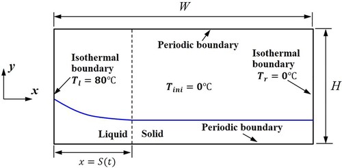
As shown in Figure 7, the computational domain is a rectangle with a length of W = 0.01 m and a height of H = 0.002 m. The density of the solid (i.e. ice) and liquid (i.e. medium water) phases is set to 1000.0 kg/m³, the thermal conductivity is set to 0.56 W/(m·°C), the heat capacity is set to 4217 J/(kg·°C), the solid melting temperature ($T_m$) is set to 0.0 °C. The latent heat of solid–liquid phase change is set to 333.4 kJ/kg. As shown in Figure 19, the initial spacing between two bubbles is set to 0.0 °C. The isothermal boundary condition is used for the left and right boundaries using five layers of virtual particles (Cleary & Monaghan, 1999). The temperature on the left and the right is fixed at 80.0 °C and 0.0 °C, respectively. The periodic boundary condition is used for the top and the bottom (Hosseini & Feng, 2011). The particle spacing is set to 0.0001m, and 20 and 100 particles are arranged along the height (y) and length (x), and a total of 2200 particles are generated, including 2000 real particles and 200 boundary particles.

Figure 7. Illustration of phase interface and temperature distribution at the time 55.5 s.

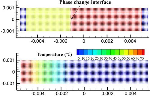
As the calculation starts, the solid phase gradually melts, and the solid–liquid interface moves from left to right. The temperature distribution in the domain and the location of the moving interface ($S\left(t\right)$) can be obtained. Figure 7 shows the phase distribution and the temperature distribution at the time of 55.5s. Figure 8 shows the time history of the phase interface position. It can be seen that the position of the interface moves along the direction of temperature gradient with time. During the heat conduction, the maximum temperature gradient decreases gradually, and the velocity of the interface also decreases.

Figure 8. The time history of the phase interface position for various temperature interval $\mathrm{\Delta }T$.

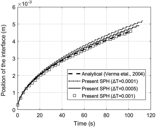
According to the phase change model, phase change occurs over a temperature range of $\mathrm{\Delta }T$. The parameter $\mathrm{\Delta }T$ is artificial (not actual). It should be small enough to approximate physical reality. However, if $\mathrm{\Delta }T$ is too small, particles might not experience phase change as the temperature can jump from a value below melting to a value above melting in one time step. Hence, a convergence study is done to determine the value of $\mathrm{\Delta }T$. In Figure 8, results using different $\mathrm{\Delta }T$ are given. It shows that the curve of S(x,t) at $\mathrm{\Delta }T$ = 0.0001 °C deviates from the theoretical solution, while the curve of 0.001 °C shows the best consistency. Hence, in this simulation, $\mathrm{\Delta }T$ is set to 0.001 °C.

4.2 Hydrostatic problem involving a solid–liquid phase change

This section focuses on the movement of the solid–liquid interface caused by the phase change in a domain containing a static fluid (Fluid 1) and a solid. As shown in Figure 9, the solid phase is below the fluid, and a solid–liquid interface exists at the initial moment. The temperature of the fluid is higher than the melting temperature of the solid, and the solid phase melts and transforms into a liquid phase (Fluid 2), creating a new fluid–fluid interface (between Fluid 1 and Fluid 2) and a new solid–liquid interface (between Fluid 2 and solid). Although this is a hydrostatic problem, the newly generated liquid phase will form a pressure gradient along the vertical direction, and the pressure field needs to be calculated by the fluid governing equation. Hence, in this simulation, both the fluid dynamics and thermal dynamics models are used.

Figure 9. Model parameters and SPH model (benchmark example 2).

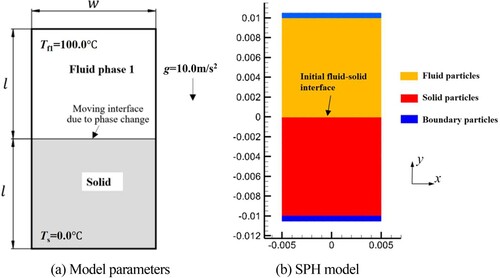
As shown in Figure 9, the upper region of the computational domain is filled with Fluid 1, and the bottom is the solid phase. The computational domain has a length of 2l ( =  0.02 m) and a width of w = 0.01 m, and the initial fluid–solid interface is located at the mid–plane (y = 0). The initial temperature of Fluid 1 is set to 100 °C, the initial temperature of the solid phase is set to 0.0 °C, and the melting temperature is set to 0.0 °C. The density of Fluid 1 is set to 100.0 kg/m³, and the dynamic viscosity is set to 0.001 N·s/m². The density of the solid and the Fluid 2 is set to 1000.0 kg/m³, and the latent heat of melting is set to 333.4 kJ/kg. The temperature interval $\mathrm{\Delta }T$ is set to 0.005 °C. The heat conductivity of both the fluid and solid phases is set to 0.56 W/(m·°C), and the specific heat capacity is set to 4217 J/(kg·°C). The surface tension is not considered in this simulation. The gravitational acceleration g is set to 10.0 m/s². Figure 9(b) shows the initialization of the SPH model. The initial particle spacing $\mathrm{\Delta }x$ is set to 0.0001 m. A total of 20 000 particles are generated. No-slip boundary (Colagrossi & Landrini, 2003) and isothermal boundary (Cleary & Monaghan, 1999) conditions are imposed on the top and bottom of the domain using five layers of virtual particles. Periodic boundary conditions are imposed on the left and right sides of the domain (Hosseini & Feng, 2011).

Figure 10 shows the results of the temperature, phase, and pressure distributions at different time instants. Initially, a large temperature gradient is present near the fluid–solid interface. The solid phase near the interface melts first and is converted to fluid phase 2. A new interface is formed between fluid phases 1 and 2. As the melting of the solid phase, the volume of fluid phase 2 increases gradually, and the fluid–solid interface moves downward. Figure 11 shows the temperature distribution along the y-direction at different time instants. Because the material absorbs latent heat during the melting process, the downward temperature gradient is lower than the upward temperature gradient. Because of gravity, a pressure gradient is formed in the fluid domain, and the maximum pressure should be located at the solid–liquid interface. Because Fluid 1 and Fluid 2 have different densities, different pressure gradients are formed in two domains. The pressure distribution along the vertical direction (i.e. y-coordinate) can be calculated in the following analytical equation: (64) $\{\begin{array}{ll}\begin{array}{l}p\left(y,t\right)={\rho }_{\text{f}2}g\left(y_{12}-y\right)\\ +{\rho }_{\text{f}1}g\left(y_{\text{top}}-y_{12}\right)\end{array}& y_{\text{ls}}\left(\text{t}\right)<\text{y}\le y_{12}\\ p\left(y,t\right)={\rho }_{\text{f}1}g\left(y_{\text{top}}-\text{y}\right)& y_{12}<\text{y}\le y_{\text{top}}\end{array},$(64) where t represents time; ${\rho }_{\text{f}1}$ and ${\rho }_{\text{f}2}$ represent the densities of Fluid 1 and Fluid 2, respectively; $y_{12}$ and $y_{\text{ls}}$ represent the y position of the fluid–fluid interface and solid–liquid interface, respectively; $y_{\text{top}}$ is the y position of the top limit of the domain. Noted that the position of the fluid–fluid interface does not change during the simulation, i.e. $y_{12}$ = 0

Figure 10. Simulation results of evolution of solid–liquid interface due to phase change.

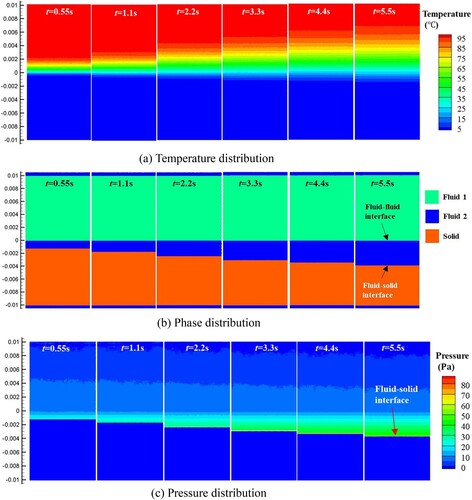
Figure 11. Temperature distributions along vertical (y) direction at different time instants.

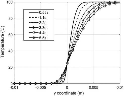
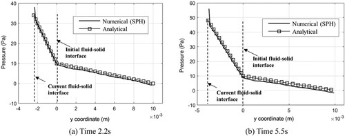
Figure 12 shows the pressure distribution of the fluid domain along the vertical direction. As shown, the pressure is zero at position y = 0.01 and increases gradually from top to bottom in a linear distribution. The pressure gradients are $-{\rho }_{f2}g$ and $-{\rho }_{f1}g$ for the domains of Fluid 2 and Fluid 1, respectively. At the solid–liquid interface, owing to the sudden transformation of solid particles to fluid particles, the pressure shows certain disturbances, but the overall distribution in the domain is linear and consistent with the analytical result.

Figure 12. Pressure distributions along vertical (y) direction.

4.3 Test of multiphase flow model

4.3.1 Square droplet deformation

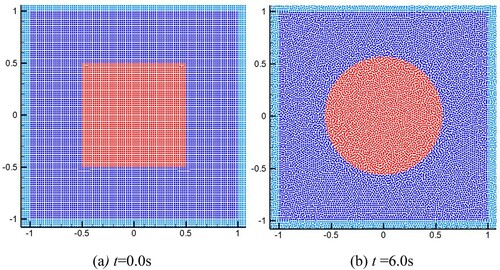
An initial square droplet will deform, contract, and oscillate due to the surface tension and will eventually evolve to the circular shape. The pressure difference between the inside and outside of the droplet converges to the Laplace pressure difference ($\mathrm{\Delta }p$), which is analytically calculated as $\mathrm{\Delta }p=\frac{\sigma }{R}$, where the parameter R is the radius of the finally circular droplet. As shown in Figure 13(a), the square droplet (Fluid 2) with the side length of 1.0 m is initially placed into a box of Fluid 1 with a domain size of 2.0 m. No-slip wall boundary condition is applied to the domain of Fluid 2 using virtual particles (Colagrossi & Landrini, 2003). The surface tension coefficient $\sigma$ is set to 1.0 N/m. The dynamic viscosity of $\mu =0.2$ N·s/m² is used for both two phases. The density of Fluid 2 is set to 1.0 kg/m³, and the density of Fluid 1 is set to 1.0 kg/m³ or 0.01 kg/m³ to obtain different density ratios (DR), 1.0 or 100.0 (we define the density ratio as the ratio of the heavy phase to the light phase). In this section, effects of the smoothing length (h) and constant of the interface sharpness force (ζ) are analysed.

Figure 13. (a) The initial particle distribution for the test of square droplet deformation, and (b) the particle distribution at t = 6.0s.

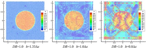
In Different values of smoothing length h are used, including 0.8$\mathrm{\Delta }x$, 1.0$\mathrm{\Delta }x$, and 1.33$\mathrm{\Delta }x$. As shown in Figure 14(a), the pressure difference curves for three smoothing lengths converge to the analytical result; however, the smaller the smoothing length, the more severe are the pressure fluctuations. As shown in Figure 15, the smoothing length of 1.33$\mathrm{\Delta }x$ corresponds to the best pressure distribution. For the smoothing length of 0.8$\mathrm{\Delta }x$, the pressure field shows the worst distribution, and the simulation is unstable. For the smoothing length of 1.0$\mathrm{\Delta }x$, although the morphology of the droplet resembles a regular circle, a certain pressure noise is presented in the domain. An excessively small smoothing length will deteriorate the accuracy and stability of the surface tension, whereas an excessively large one will increase the computing amount. The smoothing length of 1.33$\mathrm{\Delta }x$ yields the best results and is therefore used in this study.

Figure 14. Time history of pressure difference. (a) Density ratio (DR) = 1.0, showing effect of smoothing length. (b) DR = 100.0, showing effect of interface sharpness force ($\zeta$).

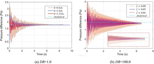
Figure 15. Pressure distributions using various smoothing lengths.

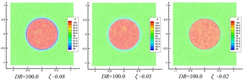
Another term that affects the accuracy and stability of surface tension is the interface sharpness force. Figure 14(b) shows the time curve of the pressure difference between the inside and outside of the droplet for different ζ. As shown, when ζis 0.05 or 0.08, the final results deviate from the analytical values. This is because the excessive interface sharpness force causes the particles on both sides of the interface to repel each other. Excessive interface sharpness force increases the distance between the particles on both sides of the interface, resulting in a decrease in the local density estimation, which consequently decreases the local pressure. As shown in Figure 16, when a smaller interface sharpness force coefficient ($\zeta$ = 0.02) is used, the non-physical reduction in pressure near the interface vanishes. Furthermore, when $\zeta$ is 0.02, an accurate surface tension is obtained and the non-physical penetration of particles under a large density ratio is also prevented. It indicates that the coefficient of the interface sharpness force should be as small as possible under the premise of ensuring the stability of the interface. The tuning procedure of the coefficient ζis one of the shortcomings of the multiphase SPH model.

Figure 16. Pressure distributions using different ζ.

4.3.2 Single bubble rising

In this section, the process of single bubble rising is simulated. An incremental inter-comparison is performed between the present SPH simulation and the simulation results in the literature (Zhang et al., 2015). In addition, the SPH results were also compared with the results of TP2D code in Hysing et al., 2009. The parameter setting uis given in Table 2, and the geometric dimensions of the computational domain are shown in Figure 17(a). The radius of the bubble (R) is set to 0.25 m. Three different particle spacings are used to discretize the computational domain, which is R/25.0, R/18.75, and R/12.5, corresponding to 20 000, 11 250, and 5000 particles, respectively. Figure 17(b) and (c) show the simulation results of the velocity distribution when the bubble morphology is stable. Figure 17(d) shows the bubble morphology at different instants (0.0–4.0 s), from which one can clearly see the dynamic process of single bubble rising.

Figure 17. (a) Model parameters of single bubble rising, and SPH results of stable bubble based on different particle spacing: (b) $\mathrm{\Delta }x=R/25.0$; (c) $\mathrm{\Delta }x=R/18.75$; (d) Bubble profiles at different time instants.

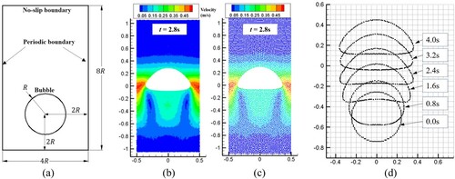
Table 2. Parameters for single bubble rising (model validation).

Fluid	Density (kg/m^3)	Viscosity (N·s/m^2)	Droplet diameter (m)	Surface tension coefficient (N/m)	Gravity acceleration (m/s^2)
Heavy phase	1000.0	10.0	0.25	24.5	0.98
Light phase	100.0	1.0

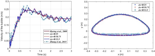
During the ascent of the bubble, the viscosity, buoyancy, and surface tension affect the deformation and motion of the bubble. The buoyancy force dominates the bubble acceleration stage, and the viscous force determines the terminal velocity of the bubble. The terminal shape of the bubble is determined by the combined effect of viscosity and surface tension. Surface tension tends to reduce the surface energy of the bubble; hence, it significantly affects the shape of the bubble. Figure 18(a) shows the velocity of the bubbles over time. Initially, the bubble accelerates; after reaching the peak velocity, the velocity of the bubble decreases slightly and then stabilizes. Although the curve predicted by the SPH model contains certain fluctuations, the overall trend is consistent with the results in literature (Hysing et al., 2009). As shown in Figure 18(b), bubble profiles obtained from different particle spacings coincide with one another, indicating that the simulation achieves the convergence.

Figure 18. (a) Time history of velocity of ascending bubble, and (b) terminal bubble morphologies using different particle spacings (t = 2.8s).

4.3.3 Two bubbles rising and coalescence

The ascent and coalescence of two bubbles is a typical example used to verify the surface tension model (Grenier et al., 2013). The parameter setting is in accordance with the literature (Colicchio, 2004) and is given in Table 3. The simulation results are compared to solutions provided by a finite-difference Navier-Stokes Level-Set solver (Colicchio, 2004).

Table 3. Physical parameters for two rising bubbles.

Fluid	Density (kg/m^3)	Viscosity (N·s/m^2)
l	1000.0	0.156
g	100.0	0.078

Before presenting the SPH simulation results, the non-dimensional Bond number (Bo) is defined as follows: (65) $Bo=\frac{{\rho }_{x}g{\left(2R\right)}^2}{\sigma },$(65) where ${\rho }_x$ represents the material density of the heavy phase; R is the small bubble radius; $\sigma$ is the surface tension coefficient.

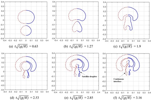
As shown in Figure 19, the initial spacing between two bubbles is set to 0.3R, R = 0.1m. The radius of the larger bubble is set to 1.5R. The initial particle spacing is set to 0.005 m, and the total number of SPH particles is 80,000. The gravitational acceleration is set to 10.0 m/s². The surface tension coefficient is set to 5.0 N/m. According to Equation (65), the Bo number is 80. Initially, the bubble is at rest; subsequently, it begins to ascend under the action of buoyancy. Figure 20 shows the SPH simulation results of the ascent and merging processes of the two bubbles. Figure 21 shows the velocity distributions at different time instants. The fluid velocity near the lower surface of the larger bubble increases and the pressure decreases correspondingly, causing an adsorption effect on the smaller bubble. Subsequently, the top of the smaller bubble elongates upwards, and the bottom forms a trailing edge, exhibiting a horseshoe shape (Figure 22(c)). The larger bubble deforms further and absorbs the smaller bubbles until a complete merge is achieved. The trailing edge of the smaller bubble detaches gradually during the ascent. Figure 22 shows a comparison between the bubble morphology obtained from the SPH simulation and the results calculated using the level-set solver. As shown, the SPH simulation results are consistent with the level-set simulation results (Colicchio, 2004; Grenier et al., 2013). Satellite droplets are formed when the trailing edge of the small bubble detaches. The SPH model can capture the formation and evolution of the satellite droplets, whereas the trailing edge interface simulated by the level-set model is continuous.

Figure 19. Schematic of two rising bubbles.

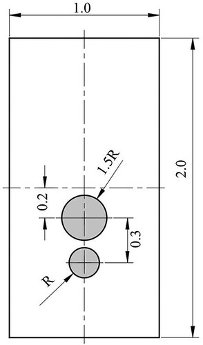
Figure 20. SPH results of two rising bubbles (Bo = 80.0).

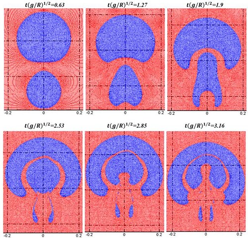
Figure 21. SPH results of two rising bubbles, showing the velocity distribution (Bo = 80.0).

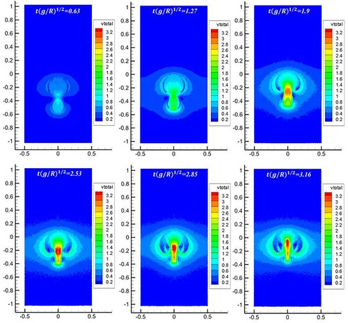
Figure 22. Comparison of bubble morphologies between present SPH results (blue line) and level-set results (dotted red line, Grenier et al., 2013) (Bo = 80.0).

5. Results and discussion

In this section, the SPH model is used to simulate the solid melting process and associated interface behavior. A total of five cases are simulated. In Section 5.1, the melting process of a square solid initially surrounded by a hot fluid is simulated without considering gravity. In Section 5.2, the melting and droplet forming process of a square solid on an adiabatic wall is simulated. In Section 5.3, the sinking and melting of a square solid in a hot fluid is simulated. This example demonstrates the ability of the model to simulate the melting of a moving object. In Section 5.4, the process of molten droplet dripping is simulated. In Section 5.5, the melting process of wax in hot water is simulated.

5.1 Case 1: melting of a square solid in a hot fluid

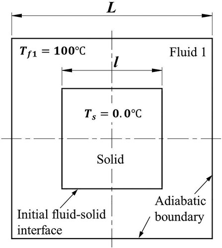
As shown in Figure 23, a square solid with a side length of l = 0.001 m is located at the domain center. The initial temperature of the ambient fluid (i.e. Fluid 1) is set to 100.0°C. The side length of the domain L is set to 0.002 m. Both the initial temperature of the solid phase and melting temperature are set to 0.0°C. The material parameters are selected according to the medium water. The thermal conductivity is set to 0.56 W/(m·°C), and the specific heat capacity to 4217 J/(kg·°C). The densities of the solid and Fluid 2 are set to 1000.0 kg/m³, and the density of Fluid 1 is set to 100 kg/m³. As the solid melts, a new fluid phase (Fluid 2) is generated. The viscosities of Fluid 1 and Fluid 2 are set to 0.001 N·s/m². The latent heat absorbed during the solid–liquid phase change is set to 333.4 kJ/kg. The surface tension coefficient is set to 0.0725 N/m. In this simulation, the solid surface is fully surrounded by the melted liquid (i.e. there is no triple contact region in the domain); thus, the wetting effect is not considered. In addition, the gravity is also not considered in thiss section.

Figure 23. Schematic of melting of a square solid (case 1).

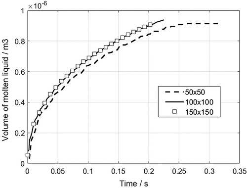
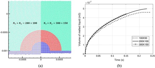
The convergence test is conducted for the particle spacing $\mathrm{\Delta }x$. Figure 24 shows the time history of the melted liquid volume with three different particle resolutions. In Figure 24, the predicted time history of melted liquid area is multiplied with a reference length (1.0m) to arrive at the volume of melted liquid. Observe that the volume–time curve obtained with a particle spacing of 0.02 mm (100 $\times$ 100) is consistent with the curve obtained with a finer particle spacing of 0.0133 mm (150 $\times$ 150). Further reduction of the particle spacing does not improve the results. Hence, a particle spacing of 0.0133 mm (150 $\times$ 150) is used.

Figure 24. The time history of melted liquid volume with three particle resolutions. The volume is obtained by multiplying the area of molten liquid by the reference length (1.0m).

Initially, owing to the temperature gradient, heat is transferred from the fluid (i.e. Fluid 1) to the solid. The solid phase begins to melt immediately and is continuously converted to Fluid 2. Because heat is transferred inward from the solid boundary, the outer part of the solid melts first, as shown in Figure 25. Meanwhile, a new phase interface is formed between Fluid 1 and Fluid 2, and the fluid near the interface begins to move because of surface tension.

Figure 25. Simulation result of the melting process of a square solid (case 1).

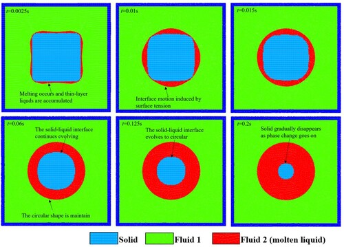
Figure 26 shows the simulation results of temperature distribution at different time instants. Initially, the temperature of the fluid surrounding the solid is higher than that of the solid. Solid particles at the four corners first melt and are converted to particles of Fluid 2. Subsequently, the outermost particles of the solid gradually melt, and a thin layer of Fluid 2 appears. As the heat conduction goes on, the square solid melts further and is finally converted into Fluid 2. The newly formed Fluid 2 finally assumes a circular shape because of surface tension.

Figure 26. Temperature distributions at different time instants (case 1).

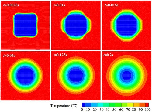
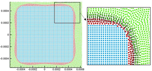
Figure 27 illustrates the normal vectors of the interface at the initial moment of the melting. As shown in Figure 27, thin liquid layers are formed and represented by several layers of fluid particles. The surface tension drives the fluid flow near the interface. Although only a small amount of Fluid 2 exist, the model can effectively calculate the surface parameters, such as the normal vector and interface curvature. Large curvatures exist at corners of the square solid, and a smoother interface can be obtained at the sharp corners with an increase in the volume of Fluid 2. The simulation results show that the SPH model can effectively simulate the phase change process (i.e. solid melting) in a multicomponent domain without any additional treatment.

Figure 27. The particle distribution and normal vector of the interface at the initial moment of melting (t = 0.0025s).

5.2 Case 2: melting of a solid with droplet formation on an adiabatic wall

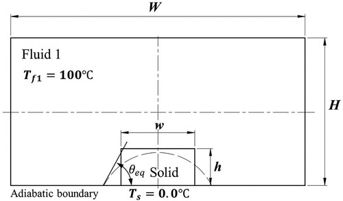
Figure 28 shows the model parameters of a rectangular solid on an adiabatic wall. As the solid melts, the melted liquid forms a droplet with a specific contact angle on the wall surface. The computing domain has a width W = 0.004 m and height H = 0.002 m. The rectangular solid has a width w = 0.001 m and height h = 0.0005 m. The initial temperature of Fluid 1 is set to 100.0°C whereas the initial temperature of the solid and melting temperature are set to 0.0°C, with a latent heat set to 333.4 kJ/kg. The thermal conductivity is set to 0.56 W/(m·°C), and the specific heat capacity to 4217 J/(kg·°C). The density of the initial fluid (Fluid 1) is set to 100.0 kg/m³, and the densities of the solid and Fluid 2 (the melted liquid) are set to 1000.0 kg/m³. The surface tension coefficient between Fluid 1 and Fluid 2 is set to 0.0725 N/m.

Figure 28. Model parameters of a square solid melting on an adiabatic wall (case 2).

The contact angle ${\theta }_{eq}$ is defined as the angle between the fluid–fluid interface and wall surface. In the SPH model, the contact angle ${\theta }_{eq}$ is an input parameter set to 90°. Based on the Young Laplace theory, for a three phase system in the equilibrium state, the following conditions are met at the three-phase contact point (Hu & Adams, 2006): (66) ${\sigma }^{f_2-s}={\sigma }^{f_2-f_1}\cos {\theta }_{eq}+{\sigma }^{f_1-s}.$(66) where ${\sigma }^{f_2-s}$, ${\sigma }^{f_2-f_1}$, and ${\sigma }^{f_1-s}$ represent the surface tension coefficients between Fluid 2 and solid, Fluid 2 and Fluid 1, and Fluid 1 and solid, respectively. From Equation (66) one can see that the expected contact angle can be obtained using different combinations of surface tension coefficients. In this section, the surface tension coefficients are set as ${\sigma }^{f_2-s}=0.0725$ N/m, ${\sigma }^{f_2-f_1}=0.0725$ N/m, and ${\sigma }^{f_1-s}=0.0725$ N/m, corresponding to the static contact angle of 90${}^{\circ }$.

The convergence test is conducted using different particle resolutions. Figure 29(a) shows that the droplet morphologies using two particle resolutions are consistent. Figure 29(b) shows the trends of the melted liquid volume are obtained with three different particle resolutions. In Figure 29(b), the predicted time history of melted liquid area is multiplied with a reference length (1.0m) to arrive at the volume of melted liquid. The result with the resolution of 200 $\times$ 100 is consistent with the curve obtained with the finer resolution of 300 $\times$ 150. Hence, the resolution of 200 $\times$ 100 is adopted.

Figure 29. (a) Comparison of droplet morphologies between two particle resolutions (t = 0.18 s), (b) trends of melted liquid volume are obtained using three particle resolutions. The volume is obtained by multiplying the area of molten liquid by the reference length (1.0m).

As shown in Figure 30, at the initial moment, the outermost layer of the solid phase melts first and the outermost solid particles change into fluid particles. There is a large curvature at the sharp corner, corresponding to a large surface tension force computed by the CSF method (Equation (49)), which disturbs the fluid near the interface (t = 0.002 s). Owing to the accumulation of molten material, a concave surface is formed at the top of the solid (t = 0.004 s). Because the surface tension always tends to ‘flatten' the fluid interface, the concave interface evolves into a ‘convex surface' (t = 0.006 s). During the process of solid melting and liquid accumulation, the evolution of the thin-layer fluid interface exhibits certain oscillations. As the melting progresses, the volume of the melted liquid gradually increases, forming a stable droplet with a spherical crown shape.

Figure 30. Simulation results of the melting process of a square solid on an adiabatic wall (case 2).

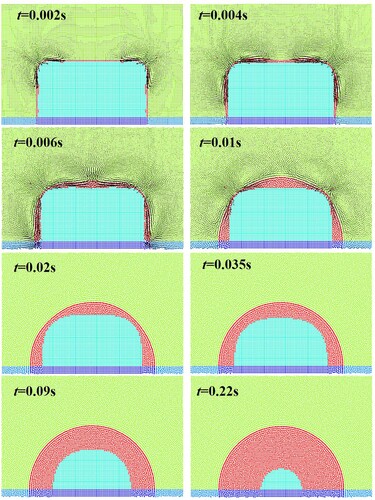
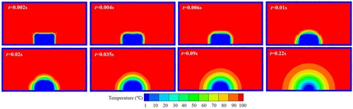
Figure 31 shows the temperature distributions of the computation domain at different time instants. The outermost particles of solid are transformed into particles of Fluid 2, leading to a new interface between Fluid 1 and Fluid 2. The solid continues to melt and the volume of Fluid 2 gradually increases. Owing to surface tension, the fluid interface evolves to minimize the surface energy. As the solid is completely melted, Fluid 2 forms a droplet with a contact angle of 90° on the surface.

Figure 31. Temperature distributions at different times (case 2).

In this simulation, the gravity is not considered, thus the morphology of the stable droplet is mainly related to the surface tension and contact angle. In our previous work, the multiphase flow SPH model was used to study the morphology of the droplet (Dong et al., 2019), where the gravity was considered. It showed that the morphology of the droplet is determined by combined effects of gravity, surface tension and contact angle. When the gravity is not considered, the shape of the stable droplet is a spherical cap, and the shape is not affected by the volume of the droplet. With considering gravity, the gravitational effect increases as the volume of the droplet increases. The shape of the droplet will no longer be a spherical cap, but will gradually become flat as the volume increases.

5.3 Case 3: sinking and melting of a solid in a hot fluid

In this section, the sinking and melting of a square solid is simulated. Figure 32 shows the model parameters for the initial configuration. The width of the computing domain W is 0.025 m and height H is 0.05 m. The side length of the square solid is set to 0.005 m. To make the melting time comparable to the sinking time, a relatively large thermal conductivity is used in this simulation. The heat conductivity is set to 2.0 W/(m·°C), with specific heat capacity of 4217.0 J/(kg·°C). The density of Fluid 1 is 500.0 kg/m³, and the density of the solid is set to 1000.0 kg/m³. The initial temperature of Fluid 1 and the solid are set to 100.0 and 0.0°C, respectively. The melting temperature of the solid is set to 0.0°C. The gravitational acceleration is set to 10.0 m/s². As the simulation begins, the solid melts and accelerates along the negative y axis direction. Based on the convergence study shown in Figure 33, the SPH particle spacing adopted in this example is 0.0001 m ($500\times 250$), and a total of 125 000 particles are used for the simulation. In Figure 33, the predicted time history of melted liquid area is multiplied with a reference length (1.0m) to arrive at the volume of melted liquid.

Figure 32. Model parameters and initial conditions of sinking and melting of a square solid (case 3).

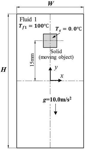
Figure 33. Time history of melted liquid volume using three different particle resolutions (case 3). The volume is obtained by multiplying the area of molten liquid by the reference length (1.0m).

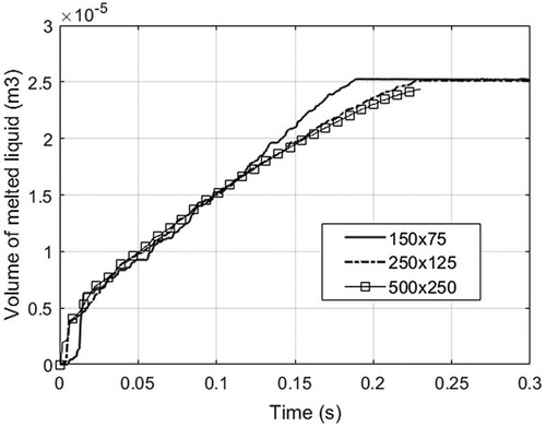
Figure 34 shows the simulation results obtained using two different particle resolutions. Notice that the generation and evolution of thin-layer fluid at the initial stage (t = 0.01 s) is significantly affected by the particle resolution. This is because no matter how small the value of the particle spacing is, the generation of molten droplets starts with a thin-layer fluid represented by a single layer of particles. However, the subsequent results show that the morphology and falling distance of the droplets obtained by the two particle resolutions are practically the same when the solid melts and forms droplets.

Figure 34. Comparison of droplet morphology between two different resolutions.

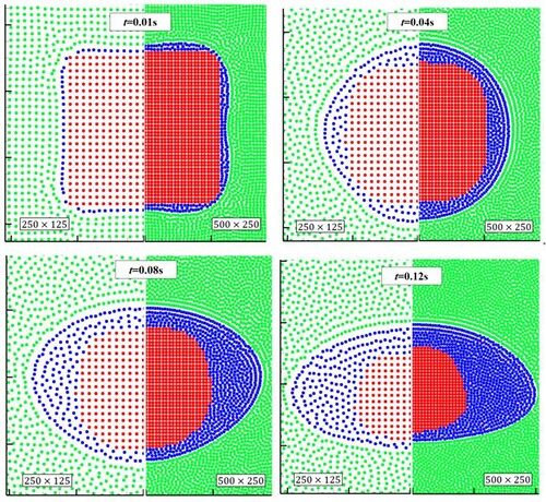
Figure 35 shows the phase, temperature, and velocity distributions at different time instants. Figure 36 shows the temperature distribution inside the melted liquid. As the density of solid material is higher than that of Fluid 1, it begins to sink due to the gravity, thus, the velocity increases from zero. Likewise, due to the presence of temperature gradient, the temperature of the solid rises, and the outermost layer of the particles melt and change into particles of Fluid 2. Initially, the melting rate is higher than the solid velocity, and the melted liquid is distributed evenly along the solid surface (0.01–0.04 s). As the settling velocity increases, the melted liquid evolves to a droplet surrounding the un-melted solid (0.08 s). The droplet gradually forms a stable flat shape as fall progresses and produces a symmetrical vortex behind it (0.12–0.20 s). Influenced by the droplet movement during the falling process, the melting rate is higher in the upper part of the solid than in other parts, and that the unmelted solid gradually evolves into a triangular shape, as shown in Figure 36.

Figure 35. SPH results of sinking and melting process of an initially square solid.

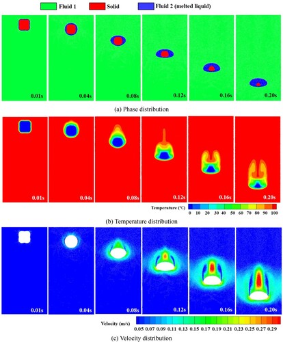
Figure 36. Temperature distribution inside the droplet during sinking of the solid. The morphology of the (unmelted) solid is shown in white (case 3).

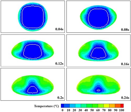
5.4 Case 4: molten droplet formation and dripping

In this section, the SPH model is used to simulate the melting process of a square solid (i.e. ice). Both the multiphase model and thermal dynamics model are used. The initial temperature distribution is shown in Figure 37. The square solid is located inside the domain and does not move during the simulation. Solid has a side length of l = 0.005 m. The side length of the entire domain is set to 0.02 m. The initial temperature of the solid and melting temperature are set to 0.0°C. The medium water is considered in this problem. The thermal conductivities of both solid and liquid phases are set to 0.56 W/(m·°C), with a fixed specific heat capacity of 4217.0 J/(kg·°C). The density of the liquid and solid is set to 100.0 and 1000.0 kg/m³, respectively, corresponding to the density ratio of 10.0. The viscosity of the two fluid phases is set to 0.001 N·s/m². The latent heat of melting is set to 333.4 kJ/kg. The gravitational acceleration is set to 10.0 m/s². Different surface tension coefficients are used to investigate the effect of Bond number. The surface tension coefficients used are 0.01, 0.005, and 0.0025 N/m corresponding to Bo numbers of 25, 50, and 100, respectively. The side length of the initial solid is used as the characteristic length for the calculation of the Bond number. The gravitational acceleration is set to 10.0 m/s².

Figure 37. Initial temperature distributions for case 4.

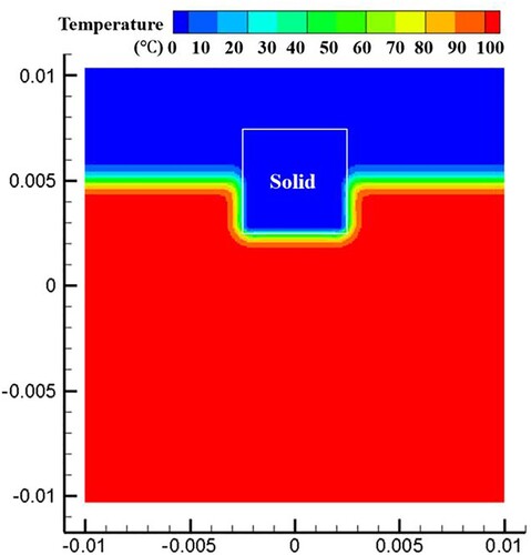
The isothermal boundary condition is used for the top and bottom boundaries using five layers of virtual particles (Cleary & Monaghan, 1999). The temperature on the top and the bottom is fixed at 0.0°C and 100.0°C, respectively. The periodic boundary condition is used for the right and the left boundaries (Hosseini & Feng, 2011). A convergence study is done regarding the simulation, as shown in Figure 38, which shows that a resolution of 300 $\times$ 300 is sufficiently fine to obtain a convergent result. More than 90,000 particles are used in the simulation.

Figure 38. (a) Time evolution of melted liquid volume with four different particle resolutions, (b) comparison of the droplet profile between two particle resolutions at time 0.22 s (the convergence study for case 4). The volume is obtained by multiplying the area of molten liquid by the reference length (1.0m).

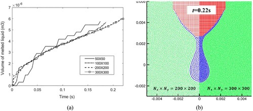
The transient process of molten droplet formation and dripping is predicted using the SPH model, as shown in Figure 39. The solid begins to melt from the bottom surface (0.003 s), and the melted liquid accumulates toward the center of the bottom surface of the solid because of gravity and surface tension (0.03 s). The volume of the melted liquid gradually increases. The growing droplet is stretched downward under gravity and maintains its intact morphology under surface tension (0.045–0.12 s). When the droplet volume increases to the point where gravity can overcome the surface tension, it produces a neck contraction and breaks, eventually forming a single droplet that drips downward (0.16–0.23 s). As the heat conduction and phase change continue, a second droplet forms and drops (0.29 s).

Figure 39. Simulation results of molten droplet formation and dripping process (case 4).

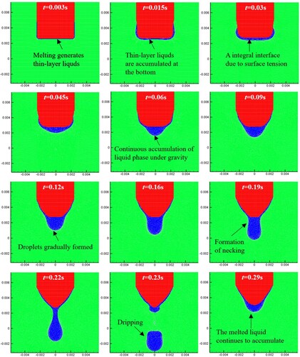
The phase change from solid to liquid absorbs the latent heat, resulting in the temperature distribution shown in Figure 40. Because of the temperature gradient, the melting interface (i.e. the solid–liquid interface) evolves into an arc shape. The particles on the solid surface are transformed into liquid particles and continuously converge into droplets. During melting process the melted liquid continues to converge, and the solid continues to form a thin layer of liquid. As the droplet volume increases, the downward velocity and convection effect of the fluid increase. Enlarged views of the droplet fragment are presented in Figure 41. The droplet has a continuous interface before dripping, after which the droplet interface deforms and breaks.

Figure 40. The temperature distribution at different time instants (case 4).

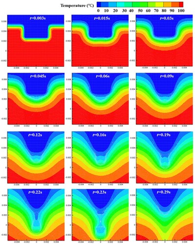
Figure 41. Droplet fragment. Arrows denote the interface normal vector.

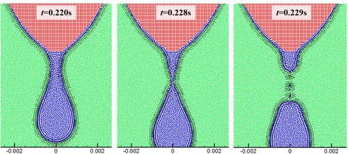
By changing the value of the surface tension coefficient $\sigma$, different Bo numbers can be set; thus, the effect of Bo number can be investigated. Three different Bond numbers are used: 25, 50, and 100. With the increase in Bo numbers, the effect of the surface tension gradually decreases. During the droplet formation and dripping, the surface tension competes with the gravity. Surface tension tends to maintain the complete interface morphology of the droplet, whereas gravity tends to break the droplet and cause the droplet to drip. As shown in Figure 42(a), for a Bo number of 25, the surface tension effect is significant. At 0.15 s, the droplet can maintain a complete shape and is in a suspended state. For a Bo number of 50.0, as shown in Figure 42(b), at 0.12 s, the droplet is in the necking stage, dripping earlier compared to the case of Bo = 25. At a Bo number of 100.0, as shown in Figure 42(c) the melted liquid on both sides of the solid forms two wave peaks (0.045 s), indicating that the surface tension cannot make the melted surface have a uniform curvature against gravity. As the Bo number increases, the time required for dripping decreases, and the melting rate of the solid increases (see Figure 43(a)). Figure 43(b) shows the relationship between the kinetic energy of the melted liquid and time with respect to different Bo numbers. As the Bo number increases, the ‘frequency' of droplet formation also increases, as well as the peak frequency of the kinetic energy curve.

Figure 42. Results of molten droplet formation and dripping process for the three different Bond numbers.

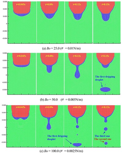
Figure 43. The time curve of melted liquid (a) volume and (b) melt kinetic energy with respect to different Bond numbers. The volume is obtained by multiplying the area of molten liquid by the reference length (1.0m).

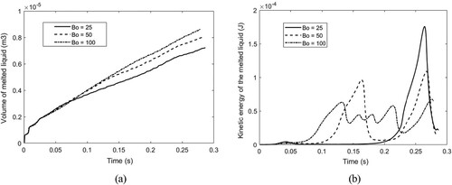
5.5 Case 5: wax melting in a tube

In this section, the SPH model is used to simulate the melting process of a wax solid in a water-filled tube. The initial model and initial temperature distributions are shown in Figure 44. The length of the computationa domain L is set to 15 mm, and the width W is set to 5 mm. The initial particle spacing $\mathrm{\Delta }x$ is set to 1/30 mm. The total number of initial solid particles and fluid particles is 67,500, and the number of boundary particles is 6100. The wax layer attached to the tube wall has a length of l = 7.5 mm and a width of w = 1.25 mm. Both the initial temperature of the solid wax and the melting temperature are set to 20.0°C. The thermal conductivity of the wax is set to 0.56 W/(m·°C), with a fixed specific heat capacity of 4217.0 J/(kg·°C). The density of water and wax are set to 1000.0 and 700.0 kg/m³, respectively. The viscosity of water and melted wax is set to 0.001 and 0.005 N·s/m², respectively. The latent heat of melting is set to 333.4 kJ/kg. The gravitational acceleration is set to 10.0 m/s². To show the effect of Bo number, different surface tension coefficients are used in the simulation, which are 6.25 $\times$ 10⁻⁴ N/m, 3.125 $\times$ 10⁻⁴ N/m, and 1.56 $\times$ 10⁻⁴ N/m. For the calculation of Bo number, the width of wax layer is used as the characteristic length.

Figure 44. Initial model of wax melting (case 5).

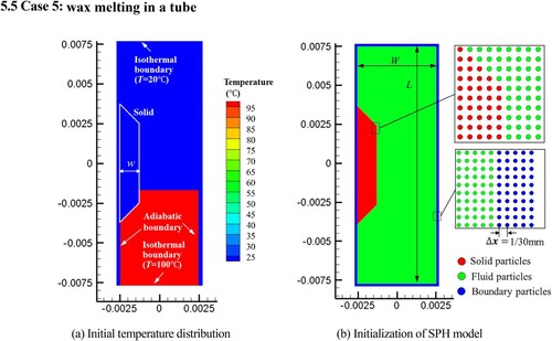
As shown in Figure 45(a), the bottom of the wax starts to melt at the initial stage. A droplet is formed and attached to the solid surface. As the volume of melted wax increases, the liquid wax moves under a combined action of surface tension, viscosity, and buoyancy. The buoyancy force causes the liquid wax to move upward, and the surface tension causes the liquid wax and surrounding water to maintain a complete interface morphology. As shown, the melted wax accumulates and gradually forms droplets as the volume increases. The droplet forms a contact angle with the solid wax layer and moves upward owing to the buoyancy force. As the volume of the droplet increases, the droplet moves away from the solid wax and becomes a separate rising bubble.

Figure 45. Simulation results of wax melting process.

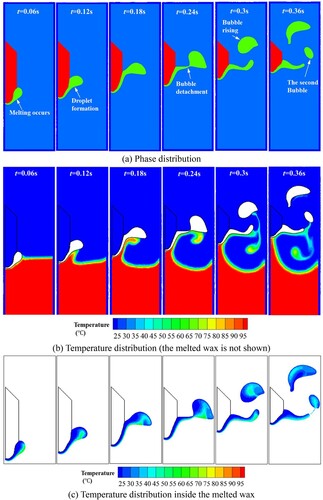
Figure 45 (b and c) show the temperature distributions in Fluid 1 and Fluid 2 at different time instants. The rising process of the droplet leads to heat convections, which accelerates the melting rate of wax. Figure 46 displays the simulation results at different Bo numbers. It shows that the smaller the Bo number, the stronger the surface tension effect, which helps maintain the complete morphology of the droplet in the initial stage of droplet formation. At a larger Bo number, the droplet detaches from the solid wax earlier.

Figure 46. Effect of Bond number on interface behaviors of melted wax.

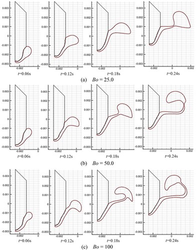
For simulating the effect of wettability, two combinations of surface tension coefficients are used. The first combination is ${\sigma }^{f_2-s}=1.0\times {10}^{-4}$ N/m, ${\sigma }^{f_2-f_1}=6.25\times {10}^{-4}$ N/m, and ${\sigma }^{f_1-s}=6.41\times {10}^{-4}$ N/m, corresponding to the contact angle of 150${}^{\circ }$. The second combination is ${\sigma }^{f_2-s}=6.41\times {10}^{-4}$ N/m, ${\sigma }^{f_2-f_1}=6.25\times {10}^{-4}$ N/m, and ${\sigma }^{f_1-s}=1.0\times {10}^{-4}$ N/m, corresponding to the contact angle of 30${}^{\circ }$. Figure 47 shows the simulation results for the two contact angles. In Figure 47(a), at ${\theta }_{eq}={150}^{\circ }$, the solid surface can not be wetted by the melted liquid, and there is a large dynamic contact angle between the droplet and solid surface (${\theta }_d>{90}^{\circ }$). In this case, the melted liquid tends to leave the solid surface as is the droplet formed. In Figure 47(b), at ${\theta }_{eq}={30}^{\circ }$, the solid surface can be wetted by the melted liquid, and a small dynamic contact angle (${\theta }_d<{90}^{\circ }$) is obtained during the melting process. As the liquid droplet forms, the droplet rises along the solid surface. The liquid droplet adheres to the solid surface, and is difficult to leave the solid surface.

Figure 47. The solid surface is (a) not wetted or (b) wetted by the melted liquid.

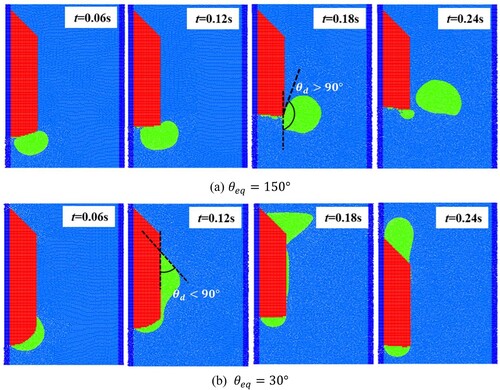
6. Conclusions

In this study, the smoothed particle hydrodynamics (SPH) method is used to simulate solid–liquid phase change problems where the domain involved solid, melted liquid, and ambient fluid. The two–dimensional SPH formulation for approximating governing equations of fluid dynamics and thermal dynamics is given with a special focus on the solid melting process and its associated interface behavior. Multicomponent problems (initially solid material surrounded by a fluid) characterized by heat transfer, melting, and multiphase fluid flow with interfacial tension are investigated.

The numerical model contains two sub-models, namely, the multiphase flow model suitable for large density ratios and thermal dynamic model involving the phase change process. The multiphase flow model includes numerical algorithms and techniques to ensure the stability of the multiphase simulation with a large density ratio. On this basis, this study simulates the wetting effect of the solid by considering the interaction between the solid, liquid, and ambient fluid. The thermal dynamic model includes a heat transfer model and a phase change model. The equivalent heat capacity method is used to quantitatively compute the latent heat absorbed or released during the phase change process, which is easy to implement in the SPH numerical flowchart.

The governing equations used in the two sub-models are discretized by the SPH formulation and are coupled to be solved by an explicit time integration algorithm. The coupling process is naturally realized in the SPH method because the SPH particles carry all the field variable information including velocity, temperature, and pressure. The solid melting process is accompanied by interface behaviors between the solid, melted liquid, and ambient fluid. These behaviors are significantly influenced by the interfacial tension, viscous force, and wetting effect. By simulating five benchmark examples and five specially configured test cases, the accuracy, robustness, convergence, and efficiency were validated and verified for real applications.

The limitations of this study: In this study, the density change due to the solid–liquid phase change was not considered, and the fluid density change caused by the thermal expansion effect was also neglected, which needs to be resolved in future work. In addition, this study only conducts the test and analysis of the two-dimensional model, and the effectiveness of the three-dimensional (3D) model needs further verification.

Disclosure statement

No potential conflict of interest was reported by the author(s).

Additional information

Funding

This work was supported by Natural Science Foundation of Shandong Province [grant number ZR2021MA039].

References

- Adami, S., Hu, X. Y., & Adams, N. A. (2010). A new surface-tension formulation for multi-phase SPH using a reproducing divergence approximation. Journal of Computational Physics, 229(13), 5011–5021. https://doi.org/10.1016/j.jcp.2010.03.022
- Adami, S., Hu, X. Y., & Adams, N. A. (2012). A generalized wall boundary condition for smoothed particle hydrodynamics. Journal of Computational Physics, 231(21), 7057–7075. https://doi.org/10.1016/j.jcp.2012.05.005
- Almasi, F., Shadloo, M. S., Hadjadj, A., Ozbulut, M., Tofighi, N., & Yildiz, M. (2019). Numerical simulations of multi-phase electro-hydrodynamics flows using a simple incompressible smoothed particle hydrodynamics method. Computers & Mathematics with Applications, 81, 772–785. https://doi.org/10.1016/j.camwa.2019.10.029
- Alshaer, A. W., Rogers, B. D., & Li, L. (2017). Smoothed particle hydrodynamics (SPH) modelling of transient heat transfer in pulsed laser ablation of Al and associated free-surface problems. Computational Materials Science, 127, 161–179. https://doi.org/10.1016/j.commatsci.2016.09.004
- Barcarolo, D. A., Le Touzé, D., Oger, G., & De Vuyst, F. (2014). Adaptive particle refinement and derefinement applied to the smoothed particle hydrodynamics method. Journal of Computational Physics, 273, 640–657. https://doi.org/10.1016/j.jcp.2014.05.040
- Batchelor, C. K. (1967). An introduction to fluid dynamics. Cambridge university press.
- Bian, X., Li, Z., & Karniadakis, G. E. (2015). Multi-resolution flow simulations by smoothed particle hydrodynamics via domain decomposition. Journal of Computational Physics, 297, 132–155. https://doi.org/10.1016/j.jcp.2015.04.044
- Bonet, J., & Lok, T. S. (1999). Variational and momentum preservation aspects of smooth particle hydrodynamic formulations. Computer Methods in Applied Mechanics and Engineering, 180(1-2), 97–115. https://doi.org/10.1016/S0045-7825(99)00051-1
- Brackbill, J. U., Kothe, D. B., & Zemach, C. (1992). A continuum method for modeling surface tension. Journal of Computational Physics, 100(2), 335–354. https://doi.org/10.1016/0021-9991(92)90240-Y
- Breinlinger, T., Polfer, P., Hashibon, A., & Kraft, T. (2013). Surface tension and wetting effects with smoothed particle hydrodynamics. Journal of Computational Physics, 243, 14–27. https://doi.org/10.1016/j.jcp.2013.02.038
- Chen, Z., Zong, Z., Liu, M. B., Zou, L., Li, H. T., & Shu, C. (2015). An SPH model for multiphase flows with complex interfaces and large density differences. Journal of Computational Physics, 283, 169–188. https://doi.org/10.1016/j.jcp.2014.11.037
- Cleary, P. W., Ha, J., Prakash, M., & Nguyen, T. (2006). 3D SPH flow predictions and validation for high pressure die casting of automotive components. Applied Mathematical Modelling, 30(11), 1406–1427. https://doi.org/10.1016/j.apm.2006.03.012
- Cleary, P. W., & Monaghan, J. J. (1999). Conduction modelling using smoothed particle hydrodynamics. Journal of Computational Physics, 148(1), 227–264. https://doi.org/10.1006/jcph.1998.6118
- Colagrossi, A., & Landrini, M. (2003). Numerical simulation of interfacial flows by smoothed particle hydrodynamics. Journal of Computational Physics, 191(2), 448–475. https://doi.org/10.1016/S0021-9991(03)00324-3
- Colicchio, G. (2004). Violent disturbance and fragmentation of free surfaces. University of Southampton.
- Dao, M. H., & Lou, J. (2021). Simulations of laser assisted additive manufacturing by smoothed particle hydrodynamics. Computer Methods in Applied Mechanics and Engineering, 373, 113491. https://doi.org/10.1016/j.cma.2020.113491
- Domínguez, J. M., Crespo, A. J. C., Gómez-Gesteira, M., & Marongiu, J. C. (2011). Neighbour lists in smoothed particle hydrodynamics. International Journal for Numerical Methods in Fluids, 67(12), 2026–2042. https://doi.org/10.1002/fld.2481
- Dong, X., Liu, J., Liu, S., & Li, Z. (2019). Quasi-static simulation of droplet morphologies using a smoothed particle hydrodynamics multiphase model. Acta Mechanica Sinica, 35(1), 32–44. https://doi.org/10.1007/s10409-018-0812-x
- Farrokhpanah, A., Bussmann, M., & Mostaghimi, J. (2017). New smoothed particle hydrodynamics (SPH) formulation for modeling heat conduction with solidification and melting. Numerical Heat Transfer, Part B: Fundamentals, 71(4), 299–312. https://doi.org/10.1080/10407790.2017.1293972
- Ferrari, A., Dumbser, M., Toro, E. F., & Armanini, A. (2009). A new 3D parallel SPH scheme for free surface flows. Computers & Fluids, 38(6), 1203–1217. https://doi.org/10.1016/j.compfluid.2008.11.012
- Frissane, H., Taddei, L., Lebaal, N., & Roth, S. (2019). SPH modeling of high velocity impact into ballistic gelatin. Development of an axis-symmetrical formulation. Mechanics of Advanced Materials and Structures, 26(22), 1881–1888. https://doi.org/10.1080/15376494.2018.1452322
- Gingold, R. A., & Monaghan, J. J. (1977). Smoothed particle hydrodynamics: Theory and application to non-spherical stars. Monthly Notices of the Royal Astronomical Society, 181(3), 375–389. https://doi.org/10.1093/mnras/181.3.375
- Glimm, J., Isaacson, E., Marchesin, D., & McBryan, O. (1981). Front tracking for hyperbolic systems. Advances in Applied Mathematics, 2(1), 91–119. https://doi.org/10.1016/0196-8858(81)90040-3
- Gnanasekaran, B., Liu, G. R., Fu, Y., Wang, G., Niu, W., & Lin, T. (2019). A smoothed particle hydrodynamics (SPH) procedure for simulating cold spray process-A study using particles. Surface and Coatings Technology, 377, 124812. https://doi.org/10.1016/j.surfcoat.2019.07.036
- Grenier, N., Antuono, M., Colagrossi, A., Le Touzé, D., & Alessandrini, B. (2009). An Hamiltonian interface SPH formulation for multi-fluid and free surface flows. Journal of Computational Physics, 228(22), 8380–8393. https://doi.org/10.1016/j.jcp.2009.08.009
- Grenier, N., Le Touzé, D., Colagrossi, A., Antuono, M., & Colicchio, G. (2013). Viscous bubbly flows simulation with an interface SPH model. Ocean Engineering, 69, 88–102. https://doi.org/10.1016/j.oceaneng.2013.05.010
- Han, L., & Hu, X. (2018). SPH modeling of fluid-structure interaction. Journal of Hydrodynamics, 30(1), 62–69. https://doi.org/10.1007/s42241-018-0006-9
- Hirt, C. W., & Nichols, B. D. (1981). Volume of fluid (vof) method for the dynamics of free boundaries. Journal of Computational Physics, 39(1), 201–225. https://doi.org/10.1016/0021-9991(81)90145-5
- Hosseini, S. M., & Feng, J. J. (2011). Pressure boundary conditions for computing incompressible flows with SPH. Journal of Computational Physics, 230(19), 7473–7487. https://doi.org/10.1016/j.jcp.2011.06.013
- Hu, X. Y., & Adams, N. A. (2006). A multi-phase SPH method for macroscopic and mesoscopic flows. Journal of Computational Physics, 213(2), 844–861. https://doi.org/10.1016/j.jcp.2005.09.001
- Huang, C., & Liu, M. B. (2020). Modeling hydrate-bearing sediment with a mixed smoothed particle hydrodynamics. Computational Mechanics, 66(4), 877–891. https://doi.org/10.1007/s00466-020-01895-1
- Hysing, S. R., Turek, S., Kuzmin, D., Parolini, N., Burman, E., Ganesan, S., & Tobiska, L. (2009). Quantitative benchmark computations of two-dimensional bubble dynamics. International Journal for Numerical Methods in Fluids, 60(11), 1259–1288. https://doi.org/10.1002/fld.1934
- Jing, H. B., & Ding, X. (2005). On criterions for smoothed particle hydrodynamics kernels in stable field. Journal of Computational Physics, 202(2), 699–709. https://doi.org/10.1016/j.jcp.2004.08.002
- Liu, G. R., & Liu, M. B. (2003). Smoothed particle hydrodynamics: A meshfree particle method. World Scientific.
- Liu, M. B., Liu, G. R., Lam, K. Y., & Zong, Z. (2003). Smoothed particle hydrodynamics for numerical simulation of underwater explosion. Computational Mechanics, 30(2), 106–118. https://doi.org/10.1007/s00466-002-0371-6
- Liu, M. B., Zhang, Z. L., & Feng, D. (2017). A density-adaptive SPH method with kernel gradient correction for modeling explosive welding. Computational Mechanics, 60(3), 513–529. https://doi.org/10.1007/s00466-017-1420-5
- Lucy, L. B. (1977). A numerical approach to the testing of the fission hypothesis. The Astronomical Journal, 82, 1013–1024. https://doi.org/10.1086/112164
- Meng, Z. F., Wang, P. P., Zhang, A. M., Ming, F. R., & Sun, P. N. (2020). A multiphase SPH model based on roe’s approximate riemann solver for hydraulic flows with complex interface. Computer Methods in Applied Mechanics and Engineering, 365, 112999. https://doi.org/10.1016/j.cma.2020.112999
- Ming, F. R., Sun, P. N., & Zhang, A. M. (2017). Numerical investigation of rising bubbles bursting at a free surface through a multiphase SPH model. Meccanica, 52(11), 2665–2684. https://doi.org/10.1007/s11012-017-0634-0
- Molteni, D., & Colagrossi, A. (2009). A simple procedure to improve the pressure evaluation in hydrodynamic context using the SPH. Computer Physics Communications, 180(6), 861–872. https://doi.org/10.1016/j.cpc.2008.12.004
- Monaghan, J. J. (1989). On the problem of penetration in particle methods. Journal of Computational Physics, 82(1), 1–15. https://doi.org/10.1016/0021-9991(89)90032-6
- Monaghan, J. J. (1994). Simulating free surface flows with SPH. Journal of Computational Physics, 110(2), 399–406. https://doi.org/10.1006/jcph.1994.1034
- Monaghan, J. J., & Gingold, R. A. (1983). Shock simulation by the particle method SPH. Journal of Computational Physics, 52(2), 374–389. https://doi.org/10.1016/0021-9991(83)90036-0
- Monaghan, J. J., Huppert, H. E., & Worster, M. G. (2005). Solidification using smoothed particle hydrodynamics. Journal of Computational Physics, 206(2), 684–705. https://doi.org/10.1016/j.jcp.2004.11.039
- Morris, J. P. (2000). Simulating surface tension with smoothed particle hydrodynamics. International Journal for Numerical Methods in Fluids, 33(3), 333–353. https://doi.org/10.1002/1097-0363(20000615)33:3<333::AID-FLD11>3.0.CO;2-7
- Morris, J. P., Fox, P. J., & Zhu, Y. (1997). Modeling low reynolds number incompressible flows using SPH. Journal of Computational Physics, 136(1), 214–226. https://doi.org/10.1006/jcph.1997.5776
- Mosavi, A., Shamshirband, S., Salwana, E., Chau, K. W., & Tah, J. H. (2019). Prediction of multi-inputs bubble column reactor using a novel hybrid model of computational fluid dynamics and machine learning. Engineering Applications of Computational Fluid Mechanics, 13(1), 482–492. https://doi.org/10.1080/19942060.2019.1613448
- Russell, M. A., Souto-Iglesias, A., & Zohdi, T. (2018). Numerical simulation of laser fusion additive manufacturing processes using the SPH method. Computer Methods in Applied Mechanics and Engineering, 341, 163–187. https://doi.org/10.1016/j.cma.2018.06.033
- Shao, J. R., Li, H. Q., Liu, G. R., & Liu, M. B. (2012). An improved SPH method for modeling liquid sloshing dynamics. Computers & Structures, 100-101, 18–26. https://doi.org/10.1016/j.compstruc.2012.02.005
- Tartakovsky, A., & Meakin, P. (2005). Modeling of surface tension and contact angles with smoothed particle hydrodynamics. Physical Review E, 72(2), 026301. https://doi.org/10.1103/PhysRevE.72.026301
- Verlet, L. (1967). Computer “experiments” on classical fluids. I. Thermodynamical properties of Lennard-Jones molecules. Physical Review, 159(1), 98. https://doi.org/10.1103/PhysRev.159.98
- Verma, A. K., Chandra, S., & Dhindaw, B. K. (2004). An alternative fixed grid method for solution of the classical one-phase Stefan problem. Applied Mathematics and Computation, 158(2), 573–584. https://doi.org/10.1016/j.amc.2003.10.001
- Viccione, G., Bovolin, V., & Carratelli, E. P. (2008). Defining and optimizing algorithms for neighbouring particle identification in SPH fluid simulations. International Journal for Numerical Methods in Fluids, 58(6), 625–638. https://doi.org/10.1002/fld.1761
- Weirather, J., Rozov, V., Wille, M., Schuler, P., Seidel, C., Adams, N. A., & Zaeh, M. F. (2019). A smoothed particle hydrodynamics model for laser beam melting of Ni-based alloy 718. Computers & Mathematics with Applications, 78(7), 2377–2394. https://doi.org/10.1016/j.camwa.2018.10.020
- Winkler, D., Rezavand, M., & Rauch, W. (2018). Neighbour lists for smoothed particle hydrodynamics on GPUs. Computer Physics Communications, 225, 140–148. https://doi.org/10.1016/j.cpc.2017.12.014
- Xia, X., & Liang, Q. (2016). A GPU-accelerated smoothed particle hydrodynamics (SPH) model for the shallow water equations. Environmental Modelling & Software, 75, 28–43. https://doi.org/10.1016/j.envsoft.2015.10.002
- Xu, R., Stansby, P., & Laurence, D. (2009). Accuracy and stability in incompressible SPH (ISPH) based on the projection method and a new approach. Journal of Computational Physics, 228(18), 6703–6725. https://doi.org/10.1016/j.jcp.2009.05.032
- Yeganehdoust, F., Yaghoubi, M., Emdad, H., & Ordoubadi, M. (2016). Numerical study of multiphase droplet dynamics and contact angles by smoothed particle hydrodynamics. Applied Mathematical Modelling, 40(19-20), 8493–8512. https://doi.org/10.1016/j.apm.2016.05.021
- Zhang, A., Sun, P., & Ming, F. (2015). An SPH modeling of bubble rising and coalescing in three dimensions. Computer Methods in Applied Mechanics and Engineering, 294, 189–209. https://doi.org/10.1016/j.cma.2015.05.014
- Zhang, A., Wen-shan, Y., & Xiong-liang, Y. (2012). Numerical simulation of underwater contact explosion. Applied Ocean Research, 34, 10–20. https://doi.org/10.1016/j.apor.2011.07.009
- Zhang, C., Rezavand, M., & Hu, X. (2021). A multi-resolution SPH method for fluid-structure interactions. Journal of Computational Physics, 429, 110028. https://doi.org/10.1016/j.jcp.2020.110028
- Zhang, M. Y., Zhang, H., & Zheng, L. L. (2008). Simulation of droplet spreading, splashing and solidification using smoothed particle hydrodynamics method. International Journal of Heat and Mass Transfer, 51(13-14), 3410–3419. https://doi.org/10.1016/j.ijheatmasstransfer.2007.11.009