Local entropy generation model for numerical CFD analysis of fluid flows through porous media, under laminar and turbulent regimes

ABSTRACT

Porous media structures have been proposed as an interesting solution on the design of high-temperature volumetric heat exchangers and sensible thermal energy storage devices. The wide exchange area between the solid matrix and the fluid offers the possibility to reach higher conversion efficiencies, particularly on applications of high-temperature (∼1000°C) gases. Nevertheless, the presence of the solid matrix increases the hydrodynamic resistance on the flow, and consequently, generates irreversibilities. The entropy generation can assess in the same figure of merit the different irreversibilities generation mechanisms. In this context, this work presents a physical and mathematical model to determine the local entropy generation (LEG) rate and recognizes its different generation mechanisms for porous media. The proposed model defines a useful expression to determine the LEG as a post-process variable from the usual CFD scalar and vectorial results (temperature, velocity, TKE, and $ϵ$), without the necessity of solving an additional entropy transport equation. A numerical experiment was implemented showing inflection points where the porous hydrodynamic resistance forces exceed the heat transfer in the LEG rate. The Forchheimer hydrodynamic resistance effect can domine the LEG in comparison to the volumetric heat transfer for high porous Reynolds regimes ($\text{R}{\text{e}}_D$>100) when the porosity is under 0.6.

KEYWORDS:

• Entropy generation
• porous media
• volumetric solar receiver
• sensible thermal energy storage
• CFD

1. Introduction

The transport phenomena between a solid porous matrix and fluid or multiphase fluid mixtures have been an active research subject during the last 70 years (Avila-Marin, 2011; Ergun & Orning, 1949; Vafai, 2015) due to their high capacity to exchange and store thermal energy (Calderón-vásquez et al., 2021; Kalita & Dass, 2011). The first interest in the literature was focused on heat exchange devices and their applications as reacting and/or filtering media (Baumann et al., 2020); however, particularly during the last 20 years, several authors have proposed novel technological solutions for energy conversion and storage systems, such as hydrogen reactors, and concentrated solar power (CSP) systems (Avila-Marin, 2011; Kribus et al., 1996, 2014; Kun-Can et al., 2017; Villafán-Vidales et al., 2011; J. Wu & Yu, 2007; Z. Wu et al., 2010, 2011; Xu et al., 2011; Younis & Viskanta, 1993). Likewise, due to the expansion of CSP systems during the last years, porous heat exchangers have been proposed as an interesting solution to increase the operating temperatures of solar tower systems using volumetric receivers. The main idea is to increase the maximum temperature of the working fluid in the solar receiver, enabling the possibility of achieving higher overall conversion efficiencies. Currently, the operation of commercial central receiver CSP systems considers a benchmark operating temperature of around ∼600°C, established by the limit of chemical stability of the working fluid: molten nitrate salts (Ho, 2016). In this context, some authors (Avila-Marin, 2011) have proposed the use of compressible gases as working fluid in combination with a porous volumetric solar receiver (VSR) to increasing the operating temperature to 1000–1200°C and, consequently, increasing the conversion efficiencies to levels of around 50% (Avila-Marin, 2011; Kribus et al., 2014). A similar idea has been proposed for thermal energy storage systems (TES) (Singh et al., 2019), using porous solid media as a sensible heat storage matrix in interaction with compressible gases. Nevertheless, the use of this kind of system implies dealing with several challenges in the design phase, mainly related to difficulties in the computational modeling stage to properly describe the transport phenomena in a complex solid porous matrix of mini- and microchannels.

Implementing a porous media either in a volumetric receiver or in a thermal storage system increases the heat exchanging area between the solid and the fluid; however, at the same time, the hydraulic resistance also increases significantly. Therefore, during the design process, it is necessary to consider a detailed analysis for determining the best configuration, material, and geometry of the porous media (i.e. ceramic foam, wire mesh, packed bed, among others), aiming to maximize the benefits of the porous morphology. In the same direction, it is necessary to have a figure of merit able to consider the trade-off of the disadvantages and the benefits in the same analysis. With this objective, some authors have proposed different approaches for assessing different materials, geometries, and designs in terms of heat exchange capacity and/or hydraulic resistance (Avila-Marin et al., 2019; Bai, 2010; Hischier et al., 2012; Z. Wu et al., 2011), showing promising results in terms of VSR technology. In 2012, Hischier et al. (Hischier et al., 2012) presented a complete analysis methodology, which defines two parameters of thermal efficiency for the concentrating and absorbing systems, respectively. Later, the authors evaluated them for several operating configurations. The results report thermal efficiencies of 90% and outlet air temperatures of 1273 K for the configuration that minimizes thermal losses. From this result, it should be interesting to extend the decision criteria and to include the concept of energy quality, as stated by the second law of thermodynamics, to include in the decision parameter the influence of the fluid temperature. A second-law analysis offers the possibility, through the entropy generation concept, to compute the irreversibilities, expressed as thermal losses and pressure drop, and the quality of the energy dispatched in terms of the outlet temperature. In 2014, Kribus et al. (Kribus et al., 2014) presented a complete review of the modeling methods and available correlations for VSR systems, considering radiative, convective, and conductive heat transfer, and pressure drop across the absorber. Nevertheless, despite the progress evidenced, the assessments still present significant discrepancies regarding the behavior of porous systems and the heat transfer capacity of porous systems. In their analysis, the authors concluded that some convective heat transfer results do not match or overestimate the heat transfer capacity of porous foams, hindering the design process and comparison with other technological proposals. Finally, the authors state that is still required additional effort in the material selection and design approaches for building structures that reach reliable high operating temperatures and conversion efficiencies. Therefore, developing a figure of merit, coupled with a detailed methodology for assessing the design of VSR systems would be significantly useful. The present study aims to describe the potential use of LEG as a metric to evaluate the performance of porous media systems, integrating thermodynamic costs in one single parameter and the loss of useful energy potential (Bejan, 1995). Through the entropy generation as a metric it is possible to assess the irreversibilities generated by the transport phenomena (mass, momentum, and energy) and, at the same time, to distinguish the best design option in terms of the quality of energy (Sarmiento et al., 2019). Thus, the proposed analysis of entropy generation offers additional information on the internal conversion processes and the rationale use of the energy resources (Bejan, 1995; Sarmiento et al., 2019).

1.1. Entropy generation in the literature

The concept of entropy generation has been widely discussed in the last 40 years (Bejan, 1980; Sciacovelli et al., 2015), and it has recently received a special emphasis due to the need for increasing the exchange and conversion and efficiencies in energy systems (Sciacovelli et al., 2015). However, despite the potential of entropy generation as a development parameter on design and optimization (Han et al., 2021; Liu et al., 2021; Song & Liu, 2018), most of the entropy generation analyses are focused on large or medium-scale systems (such as power plants or their components). On the other hand, the CFD differential-scale analyses are limited mainly to the first law of thermodynamics, focusing on the energy losses such as pressure drop and thermal losses. Nevertheless, some authors have conducted interesting studies regarding entropy generation on micro and nano scales applied to heat transfer in porous media (Betchen & Straatman, 2008; Mahian et al., 2013; Torabi et al., 2019).

In 2008, Betchen and Straatman (Betchen & Straatman, 2008) developed an entropy generation function for non-thermal equilibrium (NTE) heat transfer in high-conductivity foams using a volume-average scope in transport equations (Quintard & Whitaker, 1994). The proposed model offers an appropriate theoretical expression for the viscous dissipation entropy generation through high-conductivity foams in several realistic applications, opening pathways for novel conceptual proposals. Although Betchen and Straatman’s analysis proposes a theoretical expression for LEG in a porous foam, the results reported are restricted to laminar regimes. In addition to that, and despite their considerations, the final entropy model does not include a practical expression to determine the LEG by turbulent dissipation in terms of available turbulence models ($k-ϵ$, $k-\omega \text{SST}$, etc.) (Wilcox, 2006). Usually, the viscous dissipation effects are neglected since it does not affect significantly the entropy generation in comparison to the heat transfer. Nevertheless, turbulence has indeed an impact on the mixing and advection of heat during the exchange process.

Mahian et al. (2013) reviewed the state of the art in entropy analysis for nano fluid applications, reporting several contributions in the literature regarding differential-scale entropy analysis. The authors stated the importance of suitable relations to calculate the thermophysical properties because, in some cases, different thermophysical models could produce opposite predictions for the entropy generation. In 2010, Feng and Kleinstreuer (Feng & Kleinstreuer, 2010) presented a heat transfer analysis on parallel disc systems, using nano-fluids under laminar flow regimes. The analysis considers the entropy generation as a figure of merit, showing a comparison between the entropy generation due to viscous effects and the heat transfer, recognizing the design configurations where the viscous dissipation is negligible against the entropy variation due to heat transfer. In the same way, in 2011 Moghaddami et al. (Moghaddami et al., 2011) presented a second-law analysis over nano fluid flows through a circular pipe under laminar and turbulent regimes, varying the volume fraction of particles. The authors distinguished the dominant entropy generation mechanisms and defined the optimal design in each flow configuration.

Later in 2014, from their previous research work on LEG in porous foams (Betchen & Straatman, 2008), Betchen and Straatman (2014) conducted a pore-scale CFD analysis of high-conductivity foam heat exchangers. The analysis defines some recommendable pore geometry to maximize the heat exchange capacity by minimizing the entropy generation. Furthermore, in 2015 and based on Betchen and Straatman’s entropy generation model (Betchen & Straatman, 2008), Ting et al. (2015) presented a numerical analysis of nano fluid flows through porous media, focused on studying the relevance of viscous dissipation in the modeling of entropy generation. The authors concluded that neglecting the viscous dissipation in the analysis overestimates in 10% the fluid friction irreversibilities and underrates significantly the heat transfer irreversibilities, concluding that it is relevant to consider this effect to ensure the accuracy of the results. Recently, in 2019 Torabi et al. (Torabi et al., 2019) presented a numerical analysis of entropy generation in porous media at the pore scale. From the results, the authors show the impact on the heat exchange capacity of the porous media in terms of the diameter and shape of the pores under high Reynolds configurations. A RANS model was implemented, based on the proposal of Kock and Herwig (2004, 2005) to determine the viscous entropy generation in terms of the outlet parameters of viscous dissipation and turbulent kinetic energy (TKE) of $k-ϵ$ and $k-\omega$ turbulence models (Wilcox, 2006).

In 2005, Kock and Herwig (Kock & Herwig, 2004) presented a numerical model to link the turbulence models as $k-ϵ$ and $k-\omega$ (Wilcox, 2006) to the theoretical expression of entropy generation defined by Bejan (1995).

From the aforementioned, the LEG offers advantages on the optimization and CFD design task, in comparison with the commonly used pressure drop and heat transfer performance analysis. In that regard, an entropy generation analysis is an excellent assessing tool able to consider the trade-off between the benefit of the high heat exchanging area of porous heat exchange systems, and the thermodynamic costs of pressure drop produced by the presence of the solid matrix. Nevertheless, despite the extensive study in the literature on second-law analysis, it is necessary a LEG model able to determine the entropy generation and its generation mechanisms in fluid flows through porous matrix, from low to high Reynolds regimes. In that sense, encouraged by the wide field of applications of porous media (CSP VSR, TES, and hydrogen generation systems), and the advantages of the LEG as a figure of merit stated in the literature, the present work describes an assessment methodology for the design and optimization of heat exchange porous media systems. The proposed model allows determining the LEG for different entropy generation mechanisms (heat exchange and viscous dissipation) from high to low Reynolds regimes. The methodology determines the LEG as a post-process result from the solutions of continuity, momentum, and energy equations, without the need of solving an additional transport entropy equation per se.

Despite some authors have had analyzed the entropy generation in porous heat exchange devices (Betchen & Straatman, 2014; Torabi et al., 2017, 2019), the analyses were performed over a specific geometry of spherical or oval pores at pore-scale limiting the impact of the results under one or two types of porous geometry. Currently, several porous geometries have been proposed in the literature such as ceramic and metal foams (Capuano et al., 2016; Pabst et al., 2017; Z. Wu et al., 2010, 2011), packed wire mesh (Avila-marin, Caliot, Alvarez De Lara, et al., 2018; Avila-marin, Caliot, Flamant, et al., 2018), packed bed of rock or solid spheres (Spelling et al., 2012) and mineral wool (Fend et al., 2004), among others. Therefore, the proposed model is designed at a macroscopic scale based on the volume-averaging method (Quintard & Whitaker, 1994), with the objective of simplifying the numerical task and opening the analysis to any available geometry. Also, based on the proposal of Kock and Herwig (2004), the turbulent viscous dissipation entropy generation was determined by the available RANS turbulence models, but adapting the local entropy model to the available turbulence model developed for porous media by Nakayama and Kuwahara (1999), Pedras and De Lemos (2001), and Teruel and Rizwan-uddin (2009a, 2009b). Finally, a heat exchange of a Newtonian fluid flow through and a porous media is numerically analyzed, to identify the scope of the local entropy model.

The purpose of this work is:

• Develop a macroscopic local entropy generation expression for porous media under laminar and turbulent flow regimes, considering non-thermal equilibrium.

• Define a methodology to determine the LEG mechanisms from the CFD scalar and vectorial results (temperature, velocity, TKE, and $ϵ$).

• Analyze the LEG distribution and compare its different generation mechanisms through a numerical experiment applied to a porous channel, considering different porosities, temperature differences, and Reynolds regimes.

2. Methodology

To analyze LEG in a porous medium, the present work defines a theoretical expression for local entropy transport from low to high Reynolds regimes. Then, to determine the local entropy production due to turbulent share effects, a mathematical relation is formulated, using the scalar parameters of closure RANS turbulence models for porous media. Finally, a numerical experiment is formulated to apply the proposed theoretical model in a simple configuration. Due to the complexity associated with instrumentation in porous media, it is reasonable to perform a numerical investigation to evaluate the performance of the proposed model in an initial stage of implementation (Ghalandari et al., 2019; Salih et al., 2019).

2.1. Entropy transport from mean flux

To determine a theoretical expression for the entropy transport phenomena in porous media, the volume-averaging method (Pedras & De Lemos, 2001) is applied to the energy conservation equation. Likewise, to consider the turbulent effects related to high Reynolds regimes, the time-averaging operator is employed over the equations. As was established by Pedras and De Lemos (2001), both averaging operators (time and spatial) are independent among them (Commutative property). Therefore, the order of application of these does not modify the resulting equation or property, as follows. (1) ${〈\phi 〉}^V=\frac{1}{\Delta V}{\int }_{\Delta V}\phi \text{d}V$(1) (2) $\overline{\phi }=\frac{1}{\Delta t}{\int }_{\Delta t}\phi \text{d}\tau$(2) where $\phi$ is an auxiliary property, ${〈\phi 〉}^V$ is the average value of $\phi$ at any point inside of a representative elementary volume (REV) of size $\Delta V$, and analogously, $\overline{\phi }$ is the average value of $\phi$ in a time interval of $\Delta t$.

Thus, (3) $\begin{array}{rl}\overline{{〈\phi 〉}^V}\left(x,t\right)& =\frac{1}{\Delta t}{\int }_{\Delta t}\left(\frac{1}{\Delta V}{\int }_{\Delta V}^{}\phi \text{d}V\right)\text{d}\tau \\ & =\frac{1}{\Delta V}{\int }_{\Delta V}\left(\frac{1}{\Delta t}{\int }_{\Delta t}^{}\phi \text{d}\tau \right)\text{d}V={〈\overline{\phi }〉}^V\left(x,t\right)\end{array}$(3)

Then, the first step is to study the complete expression of the energy transport equation for a control volume (Currie, 2012), which considers the total energy per unit of mass (kinetic plus internal) and the total work done by the surface forces $\frac{\mathrm{\partial }}{\mathrm{\partial }{x}_i}\left(u_j{\sigma }_{ij}\right)$, as follows: (4) $\begin{array}{rl}& \frac{\mathrm{\partial }}{\mathrm{\partial }t}\left({\rho }_{f}e+\frac{1}{2}{\rho }_f{u}_j{u}_j\right)+\frac{\mathrm{\partial }}{\mathrm{\partial }{x}_k}\left(\left({\rho }_{f}e+\frac{1}{2}{\rho }_f{u}_j{u}_j\right)u_k\right)\\ & =\frac{\mathrm{\partial }}{\mathrm{\partial }{x}_i}\left(u_j{\sigma }_{ij}\right)+u_j{\rho }_f{f}_j-\frac{\mathrm{\partial }{q}_j}{\mathrm{\partial }{x}_j}\end{array}$(4) where ${\rho }_f$ is the fluid density, $u_j$ the fluid velocity vector, $e$ is the internal energy per unit of mass, ${\sigma }_{ij}$ the surface forces tensor, $f_j$ the mass forces vector and $q_j$ net the heat flux.

Expanding and regrouping the left-hand side terms in Equation (A1) (see the complete mathematical development in Appendix 1), it holds, (5) $\begin{array}{rl}& {\rho }_f\left[\left(\frac{\mathrm{\partial }}{\mathrm{\partial }t}\left(e\right)+\frac{\mathrm{\partial }}{\mathrm{\partial }{x}_k}\left(e\right)u_k\right)+\left(u_j\frac{\mathrm{\partial }}{\mathrm{\partial }t}\left(u_j\right)+\frac{\mathrm{\partial }}{\mathrm{\partial }{x}_k}\left(u_j\right)u_j{u}_k\right)\right]\\ & =u_j\frac{\mathrm{\partial }}{\mathrm{\partial }{x}_i}\left({\sigma }_{ij}\right)+{\sigma }_{ij}\frac{\mathrm{\partial }}{\mathrm{\partial }{x}_i}\left(u_j\right)+u_j{\rho }_f{f}_j-\frac{\mathrm{\partial }{q}_j}{\mathrm{\partial }{x}_j}\end{array}$(5)

Therefore, by applying space-averaging ${〈〉}^v$ (see the details of the volume-averaging method in Appendix 2) in Equation (5), the following expression holds, (6) $\begin{array}{rl}& {\rho }_f[\left(\frac{\mathrm{\partial }}{\mathrm{\partial }t}\left(\varphi {〈e〉}^i\right)+\varphi {〈\frac{\mathrm{\partial }}{\mathrm{\partial }{x}_k}\left(e\right)u_k〉}^i\right)\\ & +\varphi {〈\left(u_j\frac{\mathrm{\partial }}{\mathrm{\partial }t}\left(u_j\right)+\frac{\mathrm{\partial }}{\mathrm{\partial }{x}_k}\left(u_j\right)u_j{u}_k\right)〉}^i]\\ & ={〈u_j\frac{\mathrm{\partial }}{\mathrm{\partial }{x}_i}\left({\sigma }_{ij}\right)〉}^V+\varphi {〈{\sigma }_{ij}\frac{\mathrm{\partial }}{\mathrm{\partial }{x}_i}\left(u_j\right)〉}^i+\varphi {〈u_j{\rho }_f{f}_j〉}^i\\ & -[\frac{\mathrm{\partial }\left({〈q_j〉}^v\right)}{\mathrm{\partial }{x}_j}+\frac{\mathrm{\partial }}{\mathrm{\partial }{x}_j}\left(\frac{1}{\Delta V}{\int }_{A_i}\mathit{n}{\lambda }_f{T}_{f}d{s}_i\right)\\ & +\frac{1}{\Delta V}{\int }_{A_i}\mathit{n}\cdot {\lambda }_f\frac{\mathrm{\partial }{T}_f}{\mathrm{\partial }{x}_j}d{s}_i]\end{array}$(6) where ${\lambda }_f$ is the fluid conductivity and $T_f$ is the fluid temperature. In addition, the last two terms on the right-side represent the local conduction between the solid and fluid phases, and the convective heat transfer between the solid and fluid, respectively.

Expanding the first term of the right-hand side in Equation (6), and applying the space-averaging ${〈〉}^v$. (7) $\begin{array}{rl}& {〈u_j\frac{\mathrm{\partial }}{\mathrm{\partial }{x}_i}\left({\sigma }_{ij}\right)〉}^V\\ & =\varphi {〈u_j〉}^i{〈\frac{\mathrm{\partial }}{\mathrm{\partial }{x}_i}\left({\sigma }_{ij}\right)〉}^V+\varphi {〈{}^i{u}_j{\$}^i\$\left(\frac{\mathrm{\partial }}{\mathrm{\partial }{x}_i}\left({\sigma }_{ij}\right)\right)〉}^i\end{array}$(7)

Also, expanding the gradient of the surface forces tensor ${〈\frac{\mathrm{\partial }}{\mathrm{\partial }{x}_i}\left({\sigma }_{ij}\right)〉}^V$. (8) $\begin{array}{rl}& {〈\frac{\mathrm{\partial }}{\mathrm{\partial }{x}_i}\left({\sigma }_{ij}\right)〉}^V\\ & =\frac{\mathrm{\partial }}{\mathrm{\partial }{x}_i}(\phantom{\left(\varphi {〈(-P{\delta }_{ij}+\mu \left(\frac{\mathrm{\partial }{u}_i}{\mathrm{\partial }{x}_j}+\frac{\mathrm{\partial }{u}_j}{\mathrm{\partial }{x}_i}\right)-\frac{2}{3}\mu \left({\delta }_{ij}\frac{\mathrm{\partial }{u}_k}{\mathrm{\partial }{x}_k}\right))〉}^i\right)}\varphi 〈(-P{\delta }_{ij}+\mu \left(\frac{\mathrm{\partial }{u}_i}{\mathrm{\partial }{x}_j}+\frac{\mathrm{\partial }{u}_j}{\mathrm{\partial }{x}_i}\right)\\ & -{\frac{2}{3}\mu \left({\delta }_{ij}\frac{\mathrm{\partial }{u}_k}{\mathrm{\partial }{x}_k}\right))〉}^i)\\ & +\underset{\text{Darcy}\text{HR}}{\underbrace{\frac{\mu }{\Delta V}{\int }_{A_i}\left(\left(\frac{\mathrm{\partial }{u}_i}{\mathrm{\partial }{x}_j}+\frac{\mathrm{\partial }{u}_j}{\mathrm{\partial }{x}_i}\right)-\frac{2}{3}\left({\delta }_{ij}\frac{\mathrm{\partial }{u}_k}{\mathrm{\partial }{x}_k}\right)\right)\cdot \mathit{n}d{s}_i}}\\ & -\underset{\text{Forchheimer}\text{HR}}{\underbrace{\frac{1}{\Delta V}{\int }_{A_i}P\mathit{n}d{s}_i}}\end{array}$(8) where $\mu$ is the fluid viscosity, and $P$ is the pressure.

Then, the last two terms of the right-hand side in Equation (8) are the Darcy–Forchheimer’s hydrodynamic resistance terms, both related to drag forces due to the presence of the solid matrix (Pedras & De Lemos, 2001), and expressed as $R$ as follow: (9) $\begin{array}{rl}& {〈\frac{\mathrm{\partial }}{\mathrm{\partial }{x}_i}\left({\sigma }_{ij}\right)〉}^V\\ & =\frac{\mathrm{\partial }}{\mathrm{\partial }{x}_i}(-\varphi {〈P〉}^i{\delta }_{ij}+\varphi \mu (\frac{\mathrm{\partial }{〈u_i〉}^i}{\mathrm{\partial }{x}_j}+\frac{\mathrm{\partial }{〈u_j〉}^i}{\mathrm{\partial }{x}_i})\\ & -\frac{2}{3}\varphi \mu \left({\delta }_{ij}\frac{\mathrm{\partial }{〈u_k〉}^i}{\mathrm{\partial }{x}_k}\right))+R\end{array}$(9)

Then, to obtain the complete expression of the surface forces tensor ${〈u_j\frac{\mathrm{\partial }}{\mathrm{\partial }{x}_i}\left({\sigma }_{ij}\right)〉}^V$, Equation (9) is included in Equation (7), as follows. (10) $\begin{array}{rl}& {〈u_j\frac{\mathrm{\partial }}{\mathrm{\partial }{x}_i}\left({\sigma }_{ij}\right)〉}^V\\ & =\varphi {〈u_j〉}^i\frac{\mathrm{\partial }}{\mathrm{\partial }{x}_i}(-\varphi {〈P〉}^i{\delta }_{ij}+\varphi \mu \left(\frac{\mathrm{\partial }{〈u_i〉}^i}{\mathrm{\partial }{x}_j}+\frac{\mathrm{\partial }{〈u_j〉}^i}{\mathrm{\partial }{x}_i}\right)\\ & -\frac{2}{3}\varphi \mu \left({\delta }_{ij}\frac{\mathrm{\partial }{〈u_k〉}^i}{\mathrm{\partial }{x}_k}\right)\phantom{\left(\frac{\mathrm{\partial }{〈u_i〉}^i}{\mathrm{\partial }{x}_j}+\frac{\mathrm{\partial }{〈u_j〉}^i}{\mathrm{\partial }{x}_i}\right)})\\ & +\varphi {〈u_j〉}^{i}R+\varphi {〈\left({}^i\left(u_j\right){\$}^i\$\left(\frac{\mathrm{\partial }}{\mathrm{\partial }{x}_i}\left({\sigma }_{ij}\right)\right)\right)〉}^i\\ & =\varphi {〈u_j〉}^i\frac{\mathrm{\partial }}{\mathrm{\partial }{x}_i}\left(\varphi {〈{\sigma }_{ij}〉}^i\right)+\varphi {〈u_j〉}^{i}R\\ & +\varphi {〈\left({}^i\left(u_j\right){\$}^i\$\left(\frac{\mathrm{\partial }}{\mathrm{\partial }{x}_i}\left({\sigma }_{ij}\right)\right)\right)〉}^i\end{array}$(10)

Thus, introducing Equation (10) into Equation (6), (11) $\begin{array}{rl}& {\rho }_f[\left(\frac{\mathrm{\partial }}{\mathrm{\partial }t}\left(\varphi {〈e〉}^i\right)+\varphi {〈\frac{\mathrm{\partial }}{\mathrm{\partial }{x}_k}\left(e\right)u_k〉}^i\right)\\ & +\varphi {〈\left(u_j\frac{\mathrm{\partial }}{\mathrm{\partial }t}\left(u_j\right)+\frac{\mathrm{\partial }}{\mathrm{\partial }{x}_k}\left(u_j\right)u_j{u}_k\right)〉}^i]\\ & =\varphi {〈u_j〉}^i\frac{\mathrm{\partial }}{\mathrm{\partial }{x}_i}\left(\varphi {〈{\sigma }_{ij}〉}^i\right)\\ & +\varphi {〈u_j〉}^{i}R+\varphi {〈\left({}^i\left(u_j\right){\$}^i\$\left(\frac{\mathrm{\partial }}{\mathrm{\partial }{x}_i}\left({\sigma }_{ij}\right)\right)\right)〉}^i\\ & +\varphi {〈{\sigma }_{ij}\frac{\mathrm{\partial }}{\mathrm{\partial }{x}_i}\left(u_j\right)〉}^i+\varphi {〈u_j{\rho }_f{f}_j〉}^i\\ & -[\frac{\mathrm{\partial }\left({〈q_j〉}^v\right)}{\mathrm{\partial }{x}_j}+\frac{\mathrm{\partial }}{\mathrm{\partial }{x}_j}\left(\frac{1}{\Delta V}{\int }_{A_i}\mathit{n}{\lambda }_f{T}_{f}d{s}_i\right)\\ & +\frac{1}{\Delta V}{\int }_{A_i}\mathit{n}\cdot {\lambda }_f\frac{\mathrm{\partial }{T}_f}{\mathrm{\partial }{x}_j}d{s}_i]\end{array}$(11)

In Equation (11) is possible to observe that the third and fourth terms on the left-hand side are canceled by the first and third terms on the right-hand side, since these terms collectively amount to the product of $u_j$ with the momentum equation (see Appendix 3). (12) $\begin{array}{rl}& {\rho }_f\left[\left(\frac{\mathrm{\partial }}{\mathrm{\partial }t}\left(\varphi {〈e〉}^i\right)+\varphi {〈\frac{\mathrm{\partial }}{\mathrm{\partial }{x}_k}\left(e\right)u_k〉}^i\right)\right]\\ & =\varphi {〈{\sigma }_{ij}\frac{\mathrm{\partial }}{\mathrm{\partial }{x}_i}\left(u_j\right)〉}^i+\varphi {〈u_j〉}^{i}R\\ & -[\frac{\mathrm{\partial }\left({〈q_j〉}^v\right)}{\mathrm{\partial }{x}_j}+\frac{\mathrm{\partial }}{\mathrm{\partial }{x}_j}\left(\frac{1}{\Delta V}{\int }_{A_i}\mathit{n}{\lambda }_f{T}_{f}d{s}_i\right)\\ & +\frac{1}{\Delta V}{\int }_{A_i}\mathit{n}\cdot \left({\lambda }_f\frac{\mathrm{\partial }{T}_f}{\mathrm{\partial }{x}_j}\right)d{s}_i\phantom{\frac{\mathrm{\partial }\left({〈q_j〉}^v\right)}{\mathrm{\partial }{x}_j}}]\end{array}$(12)

The fourth and fifth terms on the right side correspond to the local conduction and volumetric heat transfer between the solid and fluid phases, respectively. In the literature, both heat transfer mechanisms are determined by computational simulation at pore-scale, and in some cases experimentally (Kuwahara et al., 1996). The local conduction between each phase is determined as follows (de Lemos, 2012): (13) $q_{sf,j}=\frac{1}{\Delta V}{\int }_{A_i}\mathit{n}{\lambda }_f{T}_{f}d{s}_i=-{\lambda }_{fs}\frac{\mathrm{\partial }{〈T_f〉}^i}{\mathrm{\partial }{x}_j}$(13) where ${\lambda }_{fs}$ is the local thermal conductivity tensor, usually determined by computational simulation at pore-scale. For simplicity, the local conduction term is considered inside the heat transfer term ${〈q_j〉}^v$ in the effective conductivity tensor, given by: (14) ${\lambda }_{\text{eff},f}=\varphi {\lambda }_f{\delta }_{ij}+{\lambda }_{fs}$(14)

On the other hand, the volumetric convective heat transfer is determined as a function of the temperature difference of each phase (de Lemos, 2012; Kaviany, 1999; Saito & De Lemos, 2005) as follows. (15) $\frac{1}{\Delta V}{\int }_{A_i}\mathit{n}\cdot \left({\lambda }_f\frac{\mathrm{\partial }{T}_f}{\mathrm{\partial }{x}_j}\right)d{s}_i=h_i{a}_i\left({〈T_f〉}^i-{〈T_s〉}^i\right)$(15) where $h_i$ is the interfacial convective heat transfer and $a_i$ the surface area per unit of volume.

Usually, the volumetric convection heat transfer coefficient and the local thermal conductivity tensor is determined experimentally and depends of the geometrical distribution of the solid matrix (such as packed rock bed, ceramic foam, wire mesh, etc.).

Now, for simplicity, Equation (12) is written as follows: (16) $\begin{array}{rl}& {\rho }_f\left[\left(\frac{\mathrm{\partial }}{\mathrm{\partial }t}\left(\varphi {〈e〉}^i\right)+{〈\frac{\mathrm{\partial }}{\mathrm{\partial }{x}_k}\left(e\right)u_k〉}^i\right)\right]\\ & =\varphi {〈{\sigma }_{ij}\frac{\mathrm{\partial }}{\mathrm{\partial }{x}_i}\left(u_j\right)〉}^i+\varphi {〈u_j〉}^{i}R\\ & -\frac{\mathrm{\partial }}{\mathrm{\partial }{x}_j}\left({〈q_j〉}^v\right)+h_i{a}_i\left({〈T_s〉}^i-{〈T_f〉}^i\right)\end{array}$(16)

Expanding the first term on the right-side of deformation work in Equation (16), is possible to determine the viscous dissipation term $\mathrm{\Phi }$ (Currie, 2012), as follows: (17) $\begin{array}{rl}\varphi {〈{\sigma }_{ij}\frac{\mathrm{\partial }}{\mathrm{\partial }{x}_i}\left(u_j\right)〉}^i& =\varphi 〈-P{\delta }_{ij}\frac{\mathrm{\partial }{u}_j}{\mathrm{\partial }{x}_i}+\mu \left(\frac{\mathrm{\partial }{u}_i}{\mathrm{\partial }{x}_j}+\frac{\mathrm{\partial }{u}_j}{\mathrm{\partial }{x}_i}\right)\frac{\mathrm{\partial }{u}_j}{\mathrm{\partial }{x}_i}\\ & -{\frac{2}{3}\varphi \mu \left({\delta }_{ij}\frac{\mathrm{\partial }{u}_k}{\mathrm{\partial }{x}_k}\right)\frac{\mathrm{\partial }{u}_j}{\mathrm{\partial }{x}_i}〉}^i\end{array}$(17) (18) $\begin{array}{rl}\varphi {〈{\sigma }_{ij}\frac{\mathrm{\partial }}{\mathrm{\partial }{x}_i}\left(u_j\right)〉}^i& =\varphi 〈-P\frac{\mathrm{\partial }{u}_k}{\mathrm{\partial }{x}_k}+\frac{\mu }{2}{\left(\frac{\mathrm{\partial }{u}_i}{\mathrm{\partial }{x}_j}+\frac{\mathrm{\partial }{u}_j}{\mathrm{\partial }{x}_i}\right)}^2\\ & -{\frac{2}{3}\mu {\left(\frac{\mathrm{\partial }{u}_k}{\mathrm{\partial }{x}_k}\right)}^2〉}^i\end{array}$(18) (19) $\begin{array}{rl}\varphi {〈{\sigma }_{ij}\frac{\mathrm{\partial }}{\mathrm{\partial }{x}_i}\left(u_j\right)〉}^i& =\varphi {〈-P\frac{\mathrm{\partial }{u}_k}{\mathrm{\partial }{x}_k}+\mathrm{\Phi }〉}^i\end{array}$(19)

Thus, replacing the expression (19) in Equation (16), the following expression holds, (20) $\begin{array}{rl}& {\rho }_f\left[\frac{D\left(\varphi {〈e〉}^i\right)}{Dt}\right]\\ & =-\varphi {〈P\frac{\mathrm{\partial }{u}_k}{\mathrm{\partial }{x}_k}〉}^i+\varphi {〈\mathrm{\Phi }〉}^i+\varphi {〈u_j〉}^{i}R-\frac{\mathrm{\partial }}{\mathrm{\partial }{x}_j}\left({〈q_j〉}^v\right)\\ & +h_i{a}_i\left({〈T_s〉}^i-{〈T_f〉}^i\right)\end{array}$(20)

Then, considering the continuity equation to change the term $\frac{\mathrm{\partial }{u}_k}{\mathrm{\partial }{x}_k}=-\frac{1}{{\rho }_f}\frac{D\left({\rho }_f\right)}{Dt}$ in Equation (20), and using the entropy definition from Gibbs’ equation (Bejan, 2013; Cantwell, 2018; Currie, 2012) (see Appendix 4), is possible to establish an expression for entropy transport as follows: (21) $\begin{array}{rl}& {\rho }_f\left[\frac{D\left(\varphi {〈e〉}^i\right)}{Dt}\right]\\ & =\varphi {〈P\frac{1}{{\rho }_f}\frac{D\left({\rho }_f\right)}{Dt}〉}^i+\varphi {〈\mathrm{\Phi }〉}^i+\varphi {〈u_j〉}^{i}R-\frac{\mathrm{\partial }}{\mathrm{\partial }{x}_j}\left({〈q_j〉}^v\right)\\ & +h_i{a}_i\left({〈T_s〉}^i-{〈T_f〉}^i\right)\end{array}$(21) (22) $\begin{array}{rl}& {\rho }_f\left[{〈T_f〉}^i\frac{D\left(\varphi {〈s〉}^i\right)}{Dt}\right]\\ & =-\frac{\mathrm{\partial }}{\mathrm{\partial }{x}_j}\left({〈q_j〉}^v\right)+\varphi {〈\mathrm{\Phi }〉}^i+\varphi {〈u_j〉}^{i}R\\ & +h_i{a}_i\left({〈T_s〉}^i-{〈T_f〉}^i\right)\end{array}$(22) (23) $\begin{array}{rl}& {\rho }_f\left[\frac{\mathrm{\partial }}{\mathrm{\partial }t}\left(\varphi {〈s〉}^i\right)+\varphi {〈\frac{\mathrm{\partial }}{\mathrm{\partial }{x}_k}\left(u_{k}s\right)〉}^i\right]\\ & =-\frac{1}{{〈T_f〉}^i}\frac{\mathrm{\partial }}{\mathrm{\partial }{x}_j}\left({〈q_j〉}^v\right)+\frac{\varphi {〈\mathrm{\Phi }〉}^i}{{〈T_f〉}^i}\\ & +\frac{\varphi {〈u_j〉}^i}{{〈T_f〉}^i}R+\frac{h_i{a}_i}{{〈T_f〉}^i}\left({〈T_s〉}^i-{〈T_f〉}^i\right)\end{array}$(23) where $s$ is the entropy per mass unit.

Expanding the heat transfer term on the right side of Equation (23), and using the expression $\frac{\mathrm{\partial }}{\mathrm{\partial }{x}_j}\left(\frac{q_j}{T}\right)=\frac{1}{T}\frac{\mathrm{\partial }}{\mathrm{\partial }{x}_j}\left(q_j\right)-\frac{q_j}{T^2}\frac{\mathrm{\partial }}{\mathrm{\partial }{x}_j}\left(T\right)$, (24) $\begin{array}{rl}& {\rho }_f\left[\frac{\mathrm{\partial }}{\mathrm{\partial }t}\left(\varphi {〈s〉}^i\right)+\varphi {〈\frac{\mathrm{\partial }}{\mathrm{\partial }{x}_k}\left(u_{k}s\right)〉}^i\right]\\ & =-\left(\frac{\mathrm{\partial }}{\mathrm{\partial }{x}_j}\left(\frac{{〈q_j〉}^v}{{〈T_f〉}^i}\right)+\frac{{〈q_j〉}^v}{{\left({〈T_f〉}^i\right)}^2}\frac{\mathrm{\partial }}{\mathrm{\partial }{x}_j}\left({〈T_f〉}^i\right)\right)\\ & +\frac{\varphi {〈\mathrm{\Phi }〉}^i}{{〈T_f〉}^i}+\frac{\varphi {〈u_j〉}^i}{{〈T_f〉}^i}R+\frac{h_i{a}_i}{{〈T_f〉}^i}\left({〈T_s〉}^i-{〈T_f〉}^i\right)\end{array}$(24)

In addition, it is possible to express the directional heat flux of the second term on the right-side in terms of the Fourier’s law of heat conduction (Bejan, 2013) in Equation (24) as, ${〈q_j〉}^v=-{\lambda }_{\text{eff},f}\frac{\mathrm{\partial }{〈T_f〉}^i}{\mathrm{\partial }{x}_j}$, and the right-side first term as a volumetric heat source, as follows: (25) $\begin{array}{rl}& {\rho }_f\left[\frac{\mathrm{\partial }}{\mathrm{\partial }t}\left(\varphi {〈s〉}^i\right)+\varphi {〈\frac{\mathrm{\partial }}{\mathrm{\partial }{x}_k}\left(u_{k}s\right)〉}^i\right]\\ & =-\left(\frac{\mathrm{\partial }}{\mathrm{\partial }{x}_j}\left(\frac{{〈q_j〉}^v}{{〈T_f〉}^i}\right)-\frac{{\lambda }_{\text{eff},f}}{{\left({〈T_f〉}^i\right)}^2}\frac{\mathrm{\partial }{〈T_f〉}^i}{\mathrm{\partial }{x}_j}\frac{\mathrm{\partial }{〈T_f〉}^i}{\mathrm{\partial }{x}_j}\right)\\ & +\frac{\varphi {〈\mathrm{\Phi }〉}^i}{{〈T_f〉}^i}+\frac{\varphi {〈u_j〉}^i}{{〈T_f〉}^i}R+\frac{h_i{a}_i}{{〈T_f〉}^i}\left({〈T_s〉}^i-{〈T_f〉}^i\right)\end{array}$(25) (26) $\begin{array}{rl}& {\rho }_f\left[\frac{\mathrm{\partial }}{\mathrm{\partial }t}\left(\varphi {〈s〉}^i\right)+\varphi {〈\frac{\mathrm{\partial }}{\mathrm{\partial }{x}_k}\left(u_{k}s\right)〉}^i\right]\\ & =-\frac{\mathrm{\partial }}{\mathrm{\partial }{x}_j}\left(\frac{{〈q_j〉}^v}{{〈T_f〉}^i}\right)+\frac{{\lambda }_{\text{eff},f}}{{\left({〈T_f〉}^i\right)}^2}{\left(\frac{\mathrm{\partial }{〈T_f〉}^i}{\mathrm{\partial }{x}_j}\right)}^2\\ & +\frac{\varphi {〈\mathrm{\Phi }〉}^i}{{〈T_f〉}^i}+\frac{\varphi {〈u_j〉}^i}{{〈T_f〉}^i}R+\frac{h_i{a}_i}{{〈T_f〉}^i}\left({〈T_s〉}^i-{〈T_f〉}^i\right)\end{array}$(26)

Expanding the second term of the left-side in Equation (26) the convective entropy transport due to spatial dispersion of entropy and velocity is determined as follows: (27) $\begin{array}{rl}& {\rho }_f\left[\frac{\mathrm{\partial }}{\mathrm{\partial }t}\left(\varphi {〈s〉}^i\right)+\varphi \frac{\mathrm{\partial }}{\mathrm{\partial }{x}_k}\left({〈u_k〉}^i{〈s〉}^i\right)\right]\\ & =-{\rho }_f\varphi \frac{\mathrm{\partial }}{\mathrm{\partial }{x}_k}\left({〈{}^i{u}_k{}^{i}s〉}^i\right)-\frac{\mathrm{\partial }}{\mathrm{\partial }{x}_j}\left(\frac{{〈q_j〉}^v}{{〈T_f〉}^i}\right)\\ & +\frac{{\lambda }_{\text{eff},f}}{{\left({〈T_f〉}^i\right)}^2}{\left(\frac{\mathrm{\partial }{〈T_f〉}^i}{\mathrm{\partial }{x}_j}\right)}^2\\ & +\frac{\varphi {〈\mathrm{\Phi }〉}^i}{{〈T_f〉}^i}+\frac{\varphi {〈u_j〉}^i}{{〈T_f〉}^i}R+\frac{h_i{a}_i}{{〈T_f〉}^i}\left({〈T_s〉}^i-{〈T_f〉}^i\right)\end{array}$(27)

Therefore, Equation (27) shows the local entropy transport in a porous media through a macroscopic point of view, where each term represents the following phenomena defined in Table 1.

Table 1. Local entropy transport terms.

Term	Definition
${\rho }_f\varphi {\displaystyle \frac{\mathrm{\partial }}{\mathrm{\partial }{x}_k}}\left({〈u_k〉}^i{〈s〉}^i\right)$	Convective term of microscopic advection of entropy through the spatial-mean velocity.
${\rho }_f\varphi {\displaystyle \frac{\mathrm{\partial }}{\mathrm{\partial }{x}_k}}\left({〈{}^i{u}_k{}^{i}s〉}^i\right)$	Convective entropy transport due to spatial-dispersion of entropy and velocity. This term is also present in laminar convective heat transfer, $\text{R}{\text{e}}_D<150$ (Forchheimer flow regime (Kaviany, 1999; Quintard & Whitaker, 1994)).
${\displaystyle \frac{\mathrm{\partial }}{\mathrm{\partial }{x}_j}}\left({\displaystyle \frac{{〈q_j〉}^v}{{〈T_f〉}^i}}\right)$	Macroscopic entropy generation rate due to the heat exchange between the fluid control volume and the surroundings.
${\displaystyle \frac{{\lambda }_{\text{eff},f}}{{\left({〈T_f〉}^i\right)}^2}}{\left({\displaystyle \frac{\mathrm{\partial }{〈T_f〉}^i}{\mathrm{\partial }{x}_j}}\right)}^2$	Macroscopic LEG rate by conduction heat transfer due to the spatial-mean temperature of the fluid.
${\displaystyle \frac{\varphi {〈\mathrm{\Phi }〉}^i}{{〈T_f〉}^i}}$	Macroscopic LEG rate by viscous dissipation due to spatial-mean velocity of the fluid.
${\displaystyle \frac{\varphi {〈u_j〉}^i}{{〈T_f〉}^i}}R$	Entropy generation rate due to work realized by drag efforts, related to the solid-fluid interaction.
${\displaystyle \frac{h_i{a}_i}{{〈T_f〉}^i}}\left({〈T_s〉}^i-{〈T_f〉}^i\right)$	Heat transfer entropy generation rate due to the local heat microscopic heat exchange between fluid and solid phases.

Finally, to consider turbulent effects in the analysis, the time-averaging (Reynolds et al., 1895) is applied to Equation (26), where $\overline{\phi }$ is the time average of $\phi$, as follows: (28) $\begin{array}{rl}& {\rho }_f\left[\frac{\mathrm{\partial }}{\mathrm{\partial }t}\left(\varphi {〈\overline{s}〉}^i\right)+\varphi {〈\frac{\mathrm{\partial }}{\mathrm{\partial }{x}_k}\left(\overline{u_{k}s}\right)〉}^i\right]\\ & =-\frac{\mathrm{\partial }}{\mathrm{\partial }{x}_j}\overline{\left(\frac{{〈q_j〉}^v}{{〈T_f〉}^i}\right)}+\overline{\frac{{\lambda }_{\text{eff},f}}{{\left({〈T_f〉}^i\right)}^2}{\left(\frac{\mathrm{\partial }{〈T_f〉}^i}{\mathrm{\partial }{x}_j}\right)}^2}\\ & +\overline{\frac{\varphi {〈\mathrm{\Phi }〉}^i}{{〈T_f〉}^i}}+\overline{\frac{\varphi {〈u_j〉}^i}{{〈T_f〉}^i}R}+\overline{\frac{h_i{a}_i}{{〈T_f〉}^i}\left({〈T_s〉}^i-{〈T_f〉}^i\right)}\end{array}$(28) (29) $\begin{array}{rl}& {\rho }_f\left[\frac{\mathrm{\partial }}{\mathrm{\partial }t}\left(\varphi {〈\overline{s}〉}^i\right)+\varphi {〈\frac{\mathrm{\partial }}{\mathrm{\partial }{x}_k}\left(\overline{u_{k}s}\right)〉}^i\right]\\ & =-\frac{\mathrm{\partial }}{\mathrm{\partial }{x}_j}\left(\frac{{〈\overline{q_j}〉}^v}{{〈\overline{T_f}〉}^i}\right)+\frac{{\lambda }_{\text{eff},f}}{{\left({〈\overline{T_f}〉}^i\right)}^2}\overline{{\left(\frac{\mathrm{\partial }{〈T_f〉}^i}{\mathrm{\partial }{x}_j}\right)}^2}+\frac{\varphi {〈\overline{\mathrm{\Phi }}〉}^i}{{〈\overline{T_f}〉}^i}\\ & +\frac{\varphi {〈\overline{u_j}〉}^i}{{〈\overline{T_f}〉}^i}\overline{R}+\overline{{\left(\frac{\varphi {〈u_j〉}^i}{{〈T_f〉}^i}\right)}^{\mathrm{\prime }}{R}^{\mathrm{\prime }}}+\frac{h_i{a}_i}{{〈\overline{T_f}〉}^i}\left({〈\overline{T_s}〉}^i-{〈\overline{T_f}〉}^i\right)\end{array}$(29)

Considering that the solid matrix is rigid and static, the fluctuating mechanical energy ${{〈u_j〉}^i}^{\mathrm{\prime }}{R}^{\mathrm{\prime }}$ is zero, thus, the fifth term on the right-side of Equation (29) is neglected (de Lemos, 2012; de Lemos & Pedras, 2001; Pedras & de Lemos, 2001). (30) $\begin{array}{rl}& {\rho }_f\left[\frac{\mathrm{\partial }}{\mathrm{\partial }t}\left(\varphi {〈\overline{s}〉}^i\right)+\varphi {〈\frac{\mathrm{\partial }}{\mathrm{\partial }{x}_k}\left(\overline{u_{k}s}\right)〉}^i\right]\\ & =-\frac{\mathrm{\partial }}{\mathrm{\partial }{x}_j}\left(\frac{{〈\overline{q_j}〉}^v}{{〈\overline{T_f}〉}^i}\right)+\frac{{\lambda }_{\text{eff},f}}{{\left({〈\overline{T_f}〉}^i\right)}^2}\overline{{\left(\frac{\mathrm{\partial }{〈T_f〉}^i}{\mathrm{\partial }{x}_j}\right)}^2}\\ & +\frac{\varphi {〈\overline{\mathrm{\Phi }}〉}^i}{{〈\overline{T_f}〉}^i}+\frac{\varphi {〈\overline{u_j}〉}^i}{{〈\overline{T_f}〉}^i}\overline{R}+\frac{h_i{a}_i}{{〈\overline{T_f}〉}^i}\left({〈\overline{T_s}〉}^i-{〈\overline{T_f}〉}^i\right)\end{array}$(30)

Expanding the second and third terms on the right-hand side in Equation (30), both related to entropy generation by conduction heat transfer and viscous dissipation, respectively: (31) $\begin{array}{rl}& {\rho }_f\left[\frac{\mathrm{\partial }}{\mathrm{\partial }t}\left(\varphi {〈\overline{s}〉}^i\right)+\varphi {〈\frac{\mathrm{\partial }}{\mathrm{\partial }{x}_k}\left(\overline{u_{k}s}\right)〉}^i\right]\\ & =-\frac{\mathrm{\partial }}{\mathrm{\partial }{x}_j}\left(\frac{{〈\overline{q_j}〉}^v}{{〈\overline{T_f}〉}^i}\right)\\ & +\frac{{\lambda }_{\text{eff},f}}{{\left({〈\overline{T_f}〉}^i\right)}^2}\left[{〈{\left(\frac{\mathrm{\partial }\overline{T_f}}{\mathrm{\partial }{x}_j}\right)}^2〉}^i+{〈\overline{{\left(\frac{\mathrm{\partial }{T_f}^{\mathrm{\prime }}}{\mathrm{\partial }{x}_j}\right)}^2}〉}^i\right]\\ & +\frac{2\mu \varphi }{{〈\overline{T_f}〉}^i}\left[{〈{\left(\frac{\mathrm{\partial }{\overline{u}}_i}{\mathrm{\partial }{x}_j}+\frac{\mathrm{\partial }{\overline{u}}_j}{\mathrm{\partial }{x}_i}\right)}^2+{\left(\frac{\mathrm{\partial }{\overline{u}}_k}{\mathrm{\partial }{x}_k}\right)}^2〉}^i\right]\\ & +\frac{2\mu \varphi }{{〈\overline{T_f}〉}^i}\left[{〈\overline{{\left(\frac{\mathrm{\partial }{u_i}^{\mathrm{\prime }}}{\mathrm{\partial }{x}_j}+\frac{\mathrm{\partial }{u_j}^{\mathrm{\prime }}}{\mathrm{\partial }{x}_i}\right)}^2}+\overline{{\left(\frac{\mathrm{\partial }{u_k}^{\mathrm{\prime }}}{\mathrm{\partial }{x}_k}\right)}^2}〉}^i\right]\\ & +\frac{\varphi {〈\overline{u_j}〉}^i}{{〈\overline{T_f}〉}^i}\overline{R}+\frac{h_i{a}_i}{{〈\overline{T_f}〉}^i}\left({〈\overline{T_s}〉}^i-{〈\overline{T_f}〉}^i\right)\end{array}$(31)

Finally, the LEG rate in porous media considering the effects of macroscopic turbulence is as follows: (32) $\begin{array}{rl}{〈{\dot{s}}_{\text{gen}}〉}^v& =\frac{{\lambda }_{\text{eff},f}}{{\left({〈\overline{T_f}〉}^i\right)}^2}\left[{〈{\left(\frac{\mathrm{\partial }\overline{T_f}}{\mathrm{\partial }{x}_j}\right)}^2〉}^i+{〈\overline{{\left(\frac{\mathrm{\partial }{T_f}^{\mathrm{\prime }}}{\mathrm{\partial }{x}_j}\right)}^2}〉}^i\right]\\ & +\frac{\mu \varphi }{{〈\overline{T_f}〉}^i}\left[{〈\frac{1}{2}{\left(\frac{\mathrm{\partial }{\overline{u}}_i}{\mathrm{\partial }{x}_j}+\frac{\mathrm{\partial }{\overline{u}}_j}{\mathrm{\partial }{x}_i}\right)}^2-\frac{2}{3}{\left(\frac{\mathrm{\partial }{\overline{u}}_k}{\mathrm{\partial }{x}_k}\right)}^2〉}^i\right]\\ & +\frac{\mu \varphi }{{〈\overline{T_f}〉}^i}\left[{〈\frac{1}{2}\overline{{\left(\frac{\mathrm{\partial }{u_i}^{\mathrm{\prime }}}{\mathrm{\partial }{x}_j}+\frac{\mathrm{\partial }{u_j}^{\mathrm{\prime }}}{\mathrm{\partial }{x}_i}\right)}^2}-\frac{2}{3}\overline{{\left(\frac{\mathrm{\partial }{u_k}^{\mathrm{\prime }}}{\mathrm{\partial }{x}_k}\right)}^2}〉}^i\right]\\ & +\frac{\varphi {〈\overline{u_j}〉}^i}{{〈\overline{T_f}〉}^i}\overline{R}+\frac{h_i{a}_i}{{〈\overline{T_f}〉}^i}\left({〈\overline{T_s}〉}^i-{〈\overline{T_f}〉}^i\right)\end{array}$(32)

Adding the complete expressions of the Darcy–Forchheimer analysis and the spatial-averaging method (de Lemos, 2012; Kaviany, 1999) in terms $\overline{R}$ and h_i, the entropy generation rate is: (33) $\begin{array}{rl}{〈{\dot{s}}_{\text{gen}}〉}^v& =\frac{{\lambda }_{\text{eff},f}}{{\left({〈\overline{T_f}〉}^i\right)}^2}\left[{〈{\left(\frac{\mathrm{\partial }\overline{T_f}}{\mathrm{\partial }{x}_j}\right)}^2〉}^i+{\overline{〈{\left(\frac{\mathrm{\partial }{T_f}^{\mathrm{\prime }}}{\mathrm{\partial }{x}_j}\right)}^2〉}}^i\right]\\ & +\frac{\mu \varphi }{{〈\overline{T_f}〉}^i}\left[{〈\frac{1}{2}{\left(\frac{\mathrm{\partial }{\overline{u}}_i}{\mathrm{\partial }{x}_j}+\frac{\mathrm{\partial }{\overline{u}}_j}{\mathrm{\partial }{x}_i}\right)}^2-\frac{2}{3}{\left(\frac{\mathrm{\partial }{\overline{u}}_k}{\mathrm{\partial }{x}_k}\right)}^2〉}^i\right]\\ & +\frac{\mu \varphi }{{〈\overline{T_f}〉}^i}\left[{〈\frac{1}{2}\overline{{\left(\frac{\mathrm{\partial }{u_i}^{\mathrm{\prime }}}{\mathrm{\partial }{x}_j}+\frac{\mathrm{\partial }{u_j}^{\mathrm{\prime }}}{\mathrm{\partial }{x}_i}\right)}^2}-\frac{2}{3}\overline{{\left(\frac{\mathrm{\partial }{u_k}^{\mathrm{\prime }}}{\mathrm{\partial }{x}_k}\right)}^2}〉}^i\right]\\ & +\frac{\varphi {〈\overline{u_j}〉}^i}{{〈\overline{T_f}〉}^i}[\frac{\mu }{\Delta V}{\int }_{A_i}(\left(\frac{\mathrm{\partial }{\overline{u}}_i}{\mathrm{\partial }{x}_j}+\frac{\mathrm{\partial }{\overline{u}}_j}{\mathrm{\partial }{x}_i}\right)\\ & -\frac{2}{3}\left({\delta }_{ij}\frac{\mathrm{\partial }{\overline{u}}_k}{\mathrm{\partial }{x}_k}\right))\cdot \mathit{n}d{s}_i-\frac{1}{\Delta V}{\int }_{A_i}\overline{P}\mathit{n}d{s}_i]\\ & +\frac{1}{{〈\overline{T_f}〉}^i}\left[\frac{1}{\Delta V}{\int }_{A_i}\mathit{n}\cdot {\lambda }_f\frac{\mathrm{\partial }\overline{T_f}}{\mathrm{\partial }{x}_j}d{s}_i\right]\end{array}$(33)

Rewriting the last three right-side terms as is usually in the literature from the empirical correlations, Equation (33) is as follows: (34) $\begin{array}{rl}{〈{\dot{s}}_{\text{gen}}〉}^v& =\frac{{\lambda }_{\text{eff},f}}{{\left({〈\overline{T_f}〉}^i\right)}^2}\left[{〈{\left(\frac{\mathrm{\partial }\overline{T_f}}{\mathrm{\partial }{x}_j}\right)}^2〉}^i+{\overline{〈{\left(\frac{\mathrm{\partial }{T_f}^{\mathrm{\prime }}}{\mathrm{\partial }{x}_j}\right)}^2〉}}^i\right]\\ & +\frac{\mu \varphi }{{〈\overline{T_f}〉}^i}\left[{〈\frac{1}{2}{\left(\frac{\mathrm{\partial }{\overline{u}}_i}{\mathrm{\partial }{x}_j}+\frac{\mathrm{\partial }{\overline{u}}_j}{\mathrm{\partial }{x}_i}\right)}^2-\frac{2}{3}{\left(\frac{\mathrm{\partial }{\overline{u}}_k}{\mathrm{\partial }{x}_k}\right)}^2〉}^i\right]\\ & +\frac{\mu \varphi }{{〈\overline{T_f}〉}^i}\left[{〈\frac{1}{2}\overline{{\left(\frac{\mathrm{\partial }{u_i}^{\mathrm{\prime }}}{\mathrm{\partial }{x}_j}+\frac{\mathrm{\partial }{u_j}^{\mathrm{\prime }}}{\mathrm{\partial }{x}_i}\right)}^2}-\frac{2}{3}\overline{{\left(\frac{\mathrm{\partial }{u_k}^{\mathrm{\prime }}}{\mathrm{\partial }{x}_k}\right)}^2}〉}^i\right]\\ & +\frac{\varphi }{{〈\overline{T_f}〉}^i}\left(\frac{\mu }{k_1}{\overline{u_D}}^2+\frac{{\rho }_f}{k_2}{|\overline{u_D}|}^2\overline{u_D}\right)\\ & +\frac{h_i{a}_i}{{〈\overline{T_f}〉}^i}\left({〈\overline{T_s}〉}^i-{〈\overline{T_f}〉}^i\right)\end{array}$(34) where $h_i{a}_i$, $k_1$ and $k_2$ are determined experimentally, and $u_D$ is Darcy’s velocity with $u_D=\varphi {〈\overline{u_j}〉}^i$.

Bejan presented an intuitive expression for the entropy generation in porous media under Darcian regimes ($\text{R}{\text{e}}_D$ < 1) (Bejan, 1995). In addition to this idea, Equation (34) extends the analysis to higher values of $\text{R}{\text{e}}_D$ from Darcian flow regime to post-Forchheimer and fully turbulent flow regimes, and including the LEG due to the volumetric heat transfer between the flow and the solid matrix.

Bejan’s expression: (35) ${〈{\dot{s}}_{\text{gen}}〉}^i=\frac{{\lambda }_f}{{\left({〈T_f〉}^i\right)}^2}{\left(\frac{\mathrm{\partial }{〈T_f〉}^i}{\mathrm{\partial }{x}_j}\right)}^2+\frac{{\mu }_f}{k_1{〈T_f〉}^i}{u_D}^2$(35)

In addition to Bejan’s LEG equation, in 2008 Betchen and Straatman (Betchen & Straatman, 2008) presented an extension of LEG in porous media where LEG was considered as a Forchheimer hydrodynamic resistance term and the volumetric heat transfer was included. Nevertheless, this expression was restricted to Forchheimer flow regime ($\text{R}{\text{e}}_D$ < 150). Thus, the expression developed in Equation (34) includes the LEG related to the velocity and temperature time-fluctuation effects.

2.2. Local entropy generation in turbulent share flows

Several authors (Nakayama & Kuwahara, 1999; Pedras & De Lemos, 2001; Teruel & Rizwan-uddin, 2009a, 2009b) in the literature have presented their closure models to extend the $k-ϵ$ turbulence equations scope to porous media by a macroscopic view. In general terms, the proposals have the same structure of the usual $k-ϵ$ turbulence model (Khan & Straatman, 2016). It includes an additional term in each equation related to the production and dissipation of macroscopic TKE, due to the presence of the solid matrix $G_k$ and $G_{ϵ}$ (see Table 2), as follows: (36) $\begin{array}{rl}& \frac{\mathrm{\partial }\left({\rho }_f{〈k〉}^i\right)}{\mathrm{\partial }t}+{\rho }_f\frac{\mathrm{\partial }}{\mathrm{\partial }{x}_k}\left(\overline{u_{D,k}}{〈k〉}^i\right)\\ & =-\frac{\mathrm{\partial }}{\mathrm{\partial }{x}_j}\left[\left(\mu +\frac{{\mu }_{t\varphi }}{{\sigma }_k}\right)\frac{\mathrm{\partial }}{\mathrm{\partial }{x}_j}\left(\varphi {〈k〉}^i\right)\right]\\ & +P_k-{\rho }_f\varphi {〈ϵ〉}^i+G_k\end{array}$(36) (37) $\begin{array}{rl}& \frac{\mathrm{\partial }\left({\rho }_f{〈ϵ〉}^i\right)}{\mathrm{\partial }t}+{\rho }_f\frac{\mathrm{\partial }}{\mathrm{\partial }{x}_k}\left(\overline{u_{D,k}}{〈ϵ〉}^i\right)\\ & =-\frac{\mathrm{\partial }}{\mathrm{\partial }{x}_j}\left[\left(\mu +\frac{{\mu }_{t\varphi }}{{\sigma }_k}\right)\frac{\mathrm{\partial }}{\mathrm{\partial }{x}_j}\left(\varphi {〈ϵ〉}^i\right)\right]\\ & +C_1{P}_i\frac{{〈ϵ〉}^i}{{〈k〉}^i}-C_2\frac{{〈ϵ〉}^i}{{〈k〉}^i}\left({\rho }_f\varphi {〈ϵ〉}^i\right)+G_{ϵ}\end{array}$(37) where ${〈k〉}^i$ is the volume-average TKE, ${〈ϵ〉}^i$ is the volume average of the dissipation rate of TKE, $P_i$ is the production rate of ${〈k〉}^i$, $G_i$ is the generation rate of ${〈k〉}^i$, ${\mu }_{t\varphi }$ is the turbulent viscosity for porous media, and $C_1$, $C_2$, ${\sigma }_k$ are $k$−$ϵ$ model constants.

Table 2. Volume-averaged $k-ϵ$ terms.

$G_k$	$G_{ϵ}$	Authors
$\varphi {\rho }_f{ϵ}_{\mathrm{\infty }}$	$\varphi C_{2ϵ}{\rho }_f{ϵ}_{\mathrm{\infty }}{\displaystyle \frac{{ϵ}_{\mathrm{\infty }}}{k_{\mathrm{\infty }}}}$	Nakayama and Kuwahara (Nakayama & Kuwahara, 1999)
$C_k{\rho }_f{\displaystyle \frac{\varphi k^i\overline{u_D}}{\sqrt{K}}}$	${\displaystyle \frac{\varphi C_{2ϵ}{C}_k{\rho }_f{ϵ}^i\overline{u_D}}{\sqrt{K}}}$	Pedras and de Lemos (Pedras & De Lemos, 2001)
${\displaystyle \frac{\varphi \mu \overline{u_D}}{K}}+{\displaystyle \frac{\varphi {\rho }_f{c}_E\overline{\left|\overline{u_D}\right|u_D}}{\sqrt{K}}}$	${\displaystyle \frac{\varphi f\left(\varphi ,K\right){\rho }_f{ϵ}^i\overline{u_D}}{\sqrt{K}}}$	Teruel and Rizwan-uddin (Teruel & Rizwan-uddin, 2009a, 2009b)

Therefore, to solve the usual transport equations of mass, momentum, and energy (in Appendix 5), this analysis aims to determine the LEG without solving an additional entropy transport equation. The beginning of the LEG expression determined in the previous section (Equation (34)) it is possible to define an expression of LEG as a post-process result from the velocity, temperature, TKE, and viscous dissipation results. Thus, the present analysis proposes an expression to determine the LEG as a post-process from the velocity, temperature, k, and $ϵ$ solution fields, after solving the volume-averaged conservation equations and the turbulence $k-ϵ$ equations for porous media in the literature.

Studying Equation (34) it is possible to define two principal groups of entropy generation mechanisms, heat transfer ${〈{\dot{s}}_{\mathrm{\Theta }}〉}^v$ and viscous dissipation ${〈{\dot{s}}_{\mathrm{\Phi }}〉}^v$, as follows: (38) $\begin{array}{rl}{〈{\dot{s}}_{\mathrm{\Theta }}〉}^v& =\underset{{〈{\dot{s}}_{\mathrm{\Theta },\overline{C}}〉}^v}{\underbrace{\frac{{\lambda }_{\text{eff},f}}{{\left({〈\overline{T_f}〉}^i\right)}^2}{〈{\left(\frac{\mathrm{\partial }\overline{T_f}}{\mathrm{\partial }{x}_j}\right)}^2〉}^i}}+\underset{{〈{\dot{s}}_{\mathrm{\Theta },C^{\mathrm{\prime }}}〉}^v}{\underbrace{\frac{{\lambda }_{\text{eff},f}}{{\left({〈\overline{T_f}〉}^i\right)}^2}\overline{{〈{\left(\frac{\mathrm{\partial }{T_f}^{\mathrm{\prime }}}{\mathrm{\partial }{x}_j}\right)}^2〉}^i}}}\\ & +\underset{{\dot{s}}_{\mathrm{\Theta },V}}{\underbrace{\frac{h_i{a}_i}{{〈\overline{T_f}〉}^i}\left({〈\overline{T_s}〉}^i-{〈\overline{T_f}〉}^i\right)}}\end{array}$(38) where ${〈{\dot{s}}_{\mathrm{\Theta },\overline{C}}〉}^v$ is the LEG rate by the conductive heat transfer related to the time-average fluid temperature, ${〈{\dot{s}}_{\mathrm{\Theta },C^{\mathrm{\prime }}}〉}^v$ is the LEG rate due to the conductive heat transfer associated with the fluid temperature time-fluctuations. The last term ${\dot{s}}_{\mathrm{\Theta },V}$ is the entropy generation rate, due the volumetric heat transfer between the solid and fluid phases.

Analogously, (39) $\begin{array}{rl}{〈{\dot{s}}_{\mathrm{\Phi }}〉}^v& =\underset{{〈{\dot{s}}_{\mathrm{\Phi },\overline{D}}〉}^v}{\underbrace{\frac{\mu \varphi }{{〈\overline{T_f}〉}^i}\left[{〈\frac{1}{2}{\left(\frac{\mathrm{\partial }{\overline{u}}_i}{\mathrm{\partial }{x}_j}+\frac{\mathrm{\partial }{\overline{u}}_j}{\mathrm{\partial }{x}_i}\right)}^2-\frac{2}{3}{\left(\frac{\mathrm{\partial }{\overline{u}}_k}{\mathrm{\partial }{x}_k}\right)}^2〉}^i\right]}}\\ & +\underset{{〈{\dot{s}}_{\mathrm{\Phi },D^{\mathrm{\prime }}}〉}^v}{\underbrace{\frac{\mu \varphi }{{〈\overline{T_f}〉}^i}\left[{〈\overline{\frac{1}{2}{\left(\frac{\mathrm{\partial }{u_i}^{\mathrm{\prime }}}{\mathrm{\partial }{x}_j}+\frac{\mathrm{\partial }{u_j}^{\mathrm{\prime }}}{\mathrm{\partial }{x}_i}\right)}^2}-\frac{2}{3}\overline{{\left(\frac{\mathrm{\partial }{u_k}^{\mathrm{\prime }}}{\mathrm{\partial }{x}_k}\right)}^2}〉}^i\right]}}\\ & +\underset{{\dot{s}}_{\mathrm{\Phi },DF}}{\underbrace{\frac{\varphi }{{〈\overline{T_f}〉}^i}\left(\frac{\mu }{k_1}{\overline{u_D}}^2+\frac{{\rho }_f}{k_2}{|\overline{u_D}|}^2\overline{u_D}\right)}}\end{array}$(39) where ${〈{\dot{s}}_{\mathrm{\Phi },\overline{D}}〉}^v$ is the LEG rate due to viscous dissipation related to the time-average velocity, ${〈{\dot{s}}_{\mathrm{\Phi },D^{\mathrm{\prime }}}〉}^v$ is the LEG rate by viscous dissipation regarded to the fluid velocity time-fluctuations, and ${\dot{s}}_{\mathrm{\Phi },DF}$ is the LEG rate associated to Darcy–Forchheimer’s hydrodynamic resistance due to the presence of the solid matrix against the flow.

2.2.1. Entropy generation by turbulent dissipation and thermal dispersion

For the analysis of ${〈{\dot{s}}_{\mathrm{\Phi }}〉}^v$ and ${〈{\dot{s}}_{\mathrm{\Theta }}〉}^v$, the terms ${〈{\dot{s}}_{\mathrm{\Theta },\overline{C}}〉}^v$, ${\dot{s}}_{\mathrm{\Theta },V}$ and ${〈{\dot{s}}_{\mathrm{\Phi },\overline{D}}〉}^v$ can be calculated solving the transport and volume-averaged $k-ϵ$ equations. On the other hand, the time-fluctuation terms ${〈{\dot{s}}_{\mathrm{\Phi },D^{\mathrm{\prime }}}〉}^v$ and ${〈{\dot{s}}_{\mathrm{\Theta },C^{\mathrm{\prime }}}〉}^v$, are determined from the $k-ϵ$ scalar results. Thus, from the $ϵ$ definition: (40) $\begin{array}{rl}{〈{\dot{s}}_{\mathrm{\Phi },D^{\mathrm{\prime }}}〉}^v& =\frac{\mu \varphi }{{〈\overline{T_f}〉}^i}\left[{〈\overline{\frac{1}{2}{\left(\frac{\mathrm{\partial }{u_i}^{\mathrm{\prime }}}{\mathrm{\partial }{x}_j}+\frac{\mathrm{\partial }{u_j}^{\mathrm{\prime }}}{\mathrm{\partial }{x}_i}\right)}^2}-\frac{2}{3}\overline{{\left(\frac{\mathrm{\partial }{u_k}^{\mathrm{\prime }}}{\mathrm{\partial }{x}_k}\right)}^2}〉}^i\right]\\ & =\frac{\varphi \mu {〈ϵ〉}^i}{{〈\overline{T_f}〉}^i}\end{array}$(40) where ${〈ϵ〉}^i$ is the viscous dissipation scalar term of the volume-averaged turbulence model $k-ϵ$.

To solve ${〈{\dot{s}}_{\mathrm{\Phi },D^{\mathrm{\prime }}}〉}^v$ it is necessary to consider the dissipation of the temperature time-fluctuation ${ϵ}_{\mathrm{\Theta }}={\alpha }_f\overline{{\left(\frac{\mathrm{\partial }{T_f}^{\mathrm{\prime }}}{\mathrm{\partial }{x}_j}\right)}^2}$ defined by Nagano and Kim (1988) in their two equations turbulence model, which establishes two equation pairs, $k-ϵ$ and $k_{\mathrm{\Theta }}-{ϵ}_{\mathrm{\Theta }}$, where the second defines the temperature field time-fluctuations. Thus, ${〈{\dot{s}}_{\mathrm{\Theta },C^{\mathrm{\prime }}}〉}^v$ can be rewritten as: (41) ${〈{\dot{s}}_{\mathrm{\Theta },C^{\mathrm{\prime }}}〉}^v=\frac{{\lambda }_{\text{eff},f}}{{\left({〈\overline{T_f}〉}^i\right)}^2}\overline{{〈{\left(\frac{\mathrm{\partial }{T_f}^{\mathrm{\prime }}}{\mathrm{\partial }{x}_j}\right)}^2〉}^i}=\frac{{\rho }_f{c}_{p,f}\varphi }{{\left({〈\overline{T_f}〉}^i\right)}^2}{〈{ϵ}_{\mathrm{\Theta }}〉}^i$(41)

To determine the term ${ϵ}_{\mathrm{\Theta }}$ without solving an additional $k_{\mathrm{\Theta }}-{ϵ}_{\mathrm{\Theta }}$ pair of equations, Kock and Herwig (2004) have proposed a useful approximation, which consists in approximating ${ϵ}_{\mathrm{\Theta }}$ as the production rate of $k_{\mathrm{\Theta }}$ defined as $P_{k,\mathrm{\Theta }}$ (Gersten & Herwig, 1992; Kock & Herwig, 2005). From this approximation, it is possible to determine ${ϵ}_{\mathrm{\Theta }}$ without solving an additional $k_{\mathrm{\Theta }}-{ϵ}_{\mathrm{\Theta }}$ equation system. This approximation is usually considered valid in the logarithmic region. Thus, ${ϵ}_{\mathrm{\Theta }}$ can be rewritten as follow: (42) ${\rho }_f{ϵ}_{\mathrm{\Theta }}=P_{k,\mathrm{\Theta }}=-{\rho }_f\overline{{u_j}^{\mathrm{\prime }}{T}^{\mathrm{\prime }}}\frac{\mathrm{\partial }\overline{T_f}}{\mathrm{\partial }{x}_j}$(42)

Extending Equation (42) to ${〈{ϵ}_{\mathrm{\Theta }}〉}^v$, (43) ${\rho }_f\varphi {〈{ϵ}_{\mathrm{\Theta }}〉}^i=-{\rho }_f\varphi \overline{{〈{u_j}^{\mathrm{\prime }}{T}^{\mathrm{\prime }}〉}^i}\frac{\mathrm{\partial }{〈{\overline{T}}_f〉}^i}{\mathrm{\partial }{x}_j}$(43)

In addition, to solve the terms $\overline{{〈{u_j}^{\mathrm{\prime }}{T}^{\mathrm{\prime }}〉}^i}$ a Boussinesque-like approach is applied (Kock & Herwig, 2004), adapted to the volume-average method proposed by Nakayama and Kawahara (de Lemos, 2012; Nakayama & Kuwahara, 1999), through the eddy-diffusivity concept. (44) $-\overline{{〈{u_j}^{\mathrm{\prime }}{T}^{\mathrm{\prime }}〉}^i}={\alpha }_{t\varphi }\frac{\mathrm{\partial }{〈{\overline{T}}_f〉}^i}{\mathrm{\partial }{x}_j}$(44) where ${\alpha }_{t\varphi }={\mu }_{t\varphi }/{\rho }_f\text{P}{\text{r}}_{t\varphi }$ is the turbulent thermal diffusivity for porous media, $\text{P}{\text{r}}_{t\varphi }$ is the turbulent volume-average Prandtl number, and ${\mu }_{t\varphi }$ is the turbulent viscosity for porous media ${\mu }_{t\varphi }={\rho }_f{C}_{\mu }{\left({〈k〉}^i\right)}^2/{〈ϵ〉}^i$, stated by de Lee and Howell (de Lemos, 2012; Lee & Howell, 1987).

Finally, replacing Equation (43) and Equation (44) in Equation (41): (45) $\begin{array}{rl}{〈{ϵ}_{\mathrm{\Theta }}〉}^i& =\left({\alpha }_{t\varphi }\frac{\mathrm{\partial }{〈{\overline{T}}_f〉}^i}{\mathrm{\partial }{x}_j}\right)\frac{\mathrm{\partial }{〈{\overline{T}}_f〉}^i}{\mathrm{\partial }{x}_j}\end{array}$(45) (46) $\begin{array}{rl}{〈{\dot{s}}_{\mathrm{\Theta },C^{\mathrm{\prime }}}〉}^v& =\frac{{\rho }_f{c}_{p,f}}{{\left({〈\overline{T_f}〉}^i\right)}^2}\frac{C_{\mu }{\left({〈k〉}^i\right)}^2\varphi }{P{r}_{t\varphi }{〈ϵ〉}^i}\\ & \times \left[{\left(\frac{\mathrm{\partial }{〈{\overline{T}}_f〉}^i}{\mathrm{\partial }x}\right)}^2+{\left(\frac{\mathrm{\partial }{〈{\overline{T}}_f〉}^i}{\mathrm{\partial }y}\right)}^2+{\left(\frac{\mathrm{\partial }{〈{\overline{T}}_f〉}^i}{\mathrm{\partial }z}\right)}^2\right]\end{array}$(46)

Hence, from the mathematical methodology described above it is possible to determine the LEG without solving an additional entropy transport equation or $k_{\mathrm{\Theta }}-{ϵ}_{\mathrm{\Theta }}$ equation system, additional to the usual conservation equations and $k-ϵ$ turbulence model for porous media.

Recapitulating, the proposed expression determines the LEG for a flow through a porous medium, considering the effects associated with the turbulence and the transport of heat and momentum between the solid and liquid faces. The definitive expression for the LEG and the assumptions considered are shown below.

Local entropy generation model assumptions:

• Non-thermal equilibrium between the solid and fluid phases.

• There is no mass exchange between the solid phase and the liquid phase.

• The solid matrix is rigid and static in space.

• A Newtonian fluid is considered.

• The mechanical energy of the fluctuating hydrodynamic drag force $\overline{{{〈u_j〉}^i}^{\mathrm{\prime }}{R}^{\mathrm{\prime }}}$ is neglected (de Lemos, 2012).

• The temperature time-fluctuation ${ϵ}_{\mathrm{\Theta }}$ and the production rate of $k_{\mathrm{\Theta }}$ have the same order of magnitude; ergo: ${ϵ}_{\mathrm{\Theta }}=$ $P_{k,\mathrm{\Theta }}$. (47) $\begin{array}{rl}& {〈{\dot{s}}_{\text{gen},f}〉}^v\\ & =\left(\frac{{\lambda }_{\text{eff},f}+{\lambda }_{t\varphi ,f}}{{\left({〈\overline{T_f}〉}^i\right)}^2}\right){\left(\frac{\mathrm{\partial }{〈{\overline{T}}_f〉}^i}{\mathrm{\partial }{x}_j}\right)}^2\\ & +\frac{h_i{a}_i}{{〈\overline{T_f}〉}^i}\left({〈\overline{T_s}〉}^i-{〈\overline{T_f}〉}^i\right)\\ & +\frac{\mu \varphi }{{〈\overline{T_f}〉}^i}\left[{〈\frac{1}{2}{\left(\frac{\mathrm{\partial }{\overline{u}}_i}{\mathrm{\partial }{x}_j}+\frac{\mathrm{\partial }{\overline{u}}_j}{\mathrm{\partial }{x}_i}\right)}^2-\frac{2}{3}{\left(\frac{\mathrm{\partial }{\overline{u}}_k}{\mathrm{\partial }{x}_k}\right)}^2〉}^i\right]\\ & +\frac{\varphi \mu {〈ϵ〉}^i}{{〈\overline{T_f}〉}^i}+\frac{\varphi }{{〈\overline{T_f}〉}^i}\left(\frac{\mu }{k_1}{\overline{u_D}}^2+\frac{{\rho }_f}{k_2}{|\overline{u_D}|}^2\overline{u_D}\right)\end{array}$(47)

3. Numerical experiment: study case

3.1. System description

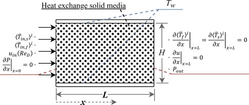
To illustrate the application of the method proposed herein, a case of study is implemented consisting of a 2D conduit, where the temperature of the solid and fluid are fixed at the entrance, as shown in Figure 1. For the entire parametrical analysis described in the following sections, the inlet fluid temperature is fixed at 300 K, and the temperature difference with the solid inlet varies from 0 to 1000 K. The temperatures of the upper and lower walls are set as the average between the solid and fluid inlet temperatures, as follows. (48) $T_w=\frac{T_{f,\text{in}}+T_{s,\text{in}}}{2}$(48)

Figure 1. Case of study diagram.

In addition, Table 3 summarizes the key physical parameters considered for the analysis.

Table 3. Analysis parameters.

	Value
System parameters
Pore diameter $\left(d_p\right)$	0.0015 m
Channel height $\left(H\right)$	0.05 m
Channel length $\left(L\right)$	0.05 m
Type of fluid	Air (Ideal Gas)
Solid medium	Ceramic Foam (Z. Wu et al., 2011)
Thermal conductivity of the solid $\left({\lambda }_s\right)$	80 Wm^−1K^−1
Simulation parameters
Fluid inlet temperature $\left({〈{\overline{T}}_{f,\text{in}}〉}^i\right)$	300 K
Solid inlet temperature $\left({〈{\overline{T}}_{s,\text{in}}〉}^i\right)$	from 301 to 1300 K
Turbulent Prandtl number$\left(\text{P}{\text{r}}_t\right)$	0.9
Outlet pressure $\left(p_{\text{out}}\right)$	101.3 kPa
Reynolds number $\left(\text{R}{\text{e}}_D\right)$	from 1 to 1000

3.2. Simulation

The channel was simulated in OpenFOAM (OpenFOAM v9, 2021) using an in-house developed solver, adapted from the porousSimpleFoam solver. This tool was built from the basic structure of the porousSimpleFoam solver, but including the solid and fluid energy equations for non-thermal equilibrium porous systems (Equation (20)). The PorousSimpleFoam tool solves the pressure and velocity from continuity and momentum equations through the SIMPLE algorithm (Semi-Implicit Method for pressure Linked Equations) of Patankar and Spalding (Patankar, 1980, 1981; Patankar & Spalding, 1972). The hydrodynamic resistance of Darcy–Forchheimer’s terms is included in the momentum equation as a source term. The turbulent effects were determined through the $k-ϵ$ tool of RAS (Reynolds average simulation) of the OpenFOAM turbulence library considering the following constants: $C_{\mu }=0.09$, ${\sigma }_k=1$, ${\sigma }_{ϵ}=1.3$, $C_{1ϵ}=1.44$, and $C_{2ϵ}=1.92$.

The simulation considers steady-state regime. The thermal conductivity and the specific heat of the fluid were determined through the correlations proposed by Z. Wu et al. (2011), and the fluid viscosity through the Sutherland law (Sutherland, 1893). Finally, the solving tolerance for the residuals was fixed to 10⁻⁷, considering a grid resolution of 500 × 1000 elements.

Assumptions for the numerical experiment modeling:

• Isotropic porosity distribution.

• The air is considered as an ideal gas.

• Steady-state regime.

• Constant thermophysical properties for the solid phase.

• The local conduction between the solid and fluid phases is neglected; ergo $\frac{\mathrm{\partial }}{\mathrm{\partial }{x}_j}\left(\frac{1}{\Delta V}{\int }_{A_i}^{}\mathit{n}{\lambda }_f{T}_{f}d{s}_i\right)=0$.

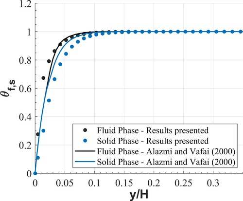
In order to validate the developed solver, a comparison was done adjusting the model parameters to the analysis presented by Alazmi and Vafai in 2000. In their analysis, several transport phenomena models for heat exchange in porous media are studied and compared. Figure 2 shows the axial profile for dimensionless temperature for each phase (fluid and solid), located at X = 0.1, where X = H/L is the dimensionless distance in the direction of flow. The results are in good agreement with those from the work of Alazmi and Vafai (2000).

Figure 2. Axial dimensionless temperature distribution considering NTE heat transfer. $\varphi =0.6$, $\text{Da}={10}^{-4}$, $d_p=0.008$, $k_s/k_f=25$, $\text{R}{\text{e}}_D=1000.$

3.3. Boundary conditions

To solve momentum and continuity equation systems, the inlet velocity and the outlet pressure are considered as fixed values. Likewise, to solve the energy equation system, the inlet and wall temperatures of the solid and fluid phases are fixed values. Finally, on the boundaries of the domain, the gradient is set to zero for the following variables, and as seen in Figure 1. (49) ${\frac{\mathrm{\partial }{u}_1}{\mathrm{\partial }x}|}_{x=L}={\frac{\mathrm{\partial }P}{\mathrm{\partial }x}|}_{x=0}={\frac{\mathrm{\partial }{〈{\overline{T}}_f〉}^i}{\mathrm{\partial }x}|}_{x=L}={\frac{\mathrm{\partial }{〈{\overline{T}}_s〉}^i}{\mathrm{\partial }x}|}_{x=L}=0$(49)

3.4. Dimensionless analysis

As a prelude of the numerical analysis, to have more information about the relevance of each LEG mechanism before the CFD analysis, a dimensionless analysis was developed considering the following dimensionless variables: $\begin{array}{rl}{}^{\ast }{x}_i& =\frac{x_i}{H},{}^{\ast }{\overline{u}}_i=\frac{{\overline{u}}_i}{U_0}\\ {\theta }_f& =\frac{T_f-T_{f,\text{in}}}{T_w-T_{f,\text{in}}},{\gamma }_f=\frac{T_{f,\text{in}}}{T_w-T_{f,\text{in}}}\\ {\theta }_s& =\frac{T_s-T_{s,\text{in}}}{T_w-T_{s,\text{in}}},{\gamma }_s=\frac{T_{s,\text{in}}}{T_w-T_{s,\text{in}}}\end{array}$where ${}^{\ast }{x}_i$ is the dimensionless longitude, ${}^{\ast }{\overline{u}}_i$ is the dimensionless velocity, $\theta$ is the dimensionless temperature difference, and $\gamma$ is the dimensionless inlet temperature. The subscripts f and s denote the fluid and solid phases, respectively. Thus, as was proposed by Betchen and Straatman (2008), the dimensionless LEG term is written as follows: (50) $\begin{array}{rl}{}^{\ast }{〈{\dot{s}}_{\text{gen},f}〉}^v& =\frac{{〈{\dot{s}}_{\text{gen},f}〉}^v{H}^2}{{\lambda }_f}\end{array}$(50) (51) $\begin{array}{rl}{}^{\ast }{〈{\dot{s}}_{\text{gen},f}〉}^v& ={}^{\ast }{〈{\dot{s}}_{\mathrm{\Theta },\overline{C}}〉}^v+{}^{\ast }{〈{\dot{s}}_{\mathrm{\Theta },C^{\mathrm{\prime }}}〉}^v+{}^{\ast }{\dot{s}}_{\mathrm{\Theta },V}\\ & +{}^{\ast }{〈{\dot{s}}_{\mathrm{\Phi },\overline{D}}〉}^v+{}^{\ast }{〈{\dot{s}}_{\mathrm{\Phi },D^{\mathrm{\prime }}}〉}^v+{}^{\ast }{\dot{s}}_{\mathrm{\Phi },DF}\end{array}$(51) where ${}^{\ast }\left(\right)$ refers to a dimensionless expression.

Then, substituting the dimensionless properties on Equation (38). (52) $\begin{array}{rl}& {}^{\ast }{〈{\dot{s}}_{\mathrm{\Theta },\overline{C}}〉}^v+{}^{\ast }{〈{\dot{s}}_{\mathrm{\Theta },C^{\mathrm{\prime }}}〉}^v+{}^{\ast }{\dot{s}}_{\mathrm{\Theta },V}\\ & =\left(\frac{\varphi {\lambda }_f{H}^2}{{\lambda }_f{\left({\theta }_f+{\gamma }_f\right)}^2{H}^2}+\frac{{\rho }_f{c}_{p,f}{\mu }_{t\varphi }{H}^2}{{\lambda }_f{\left({\theta }_f+{\gamma }_f\right)}^2{H}^2}\right)\\ & \times \left[{\left(\frac{\mathrm{\partial }{\theta }_f}{{\mathrm{\partial }}^{\ast }x}\right)}^2+{\left(\frac{\mathrm{\partial }{\theta }_f}{{\mathrm{\partial }}^{\ast }y}\right)}^2+{\left(\frac{\mathrm{\partial }{\theta }_f}{{\mathrm{\partial }}^{\ast }z}\right)}^2\right]\\ & +\frac{h_i{a}_i{H}^2}{{\lambda }_f\left({\theta }_f+{\gamma }_f\right)}\left[\left({\theta }_s+{\gamma }_s\right)-\left({\theta }_f+{\gamma }_f\right)\right]\end{array}$(52)

Regrouping terms, (53) $\begin{array}{rl}& {}^{\ast }{〈{\dot{s}}_{\mathrm{\Theta },\overline{C}}〉}^v+{}^{\ast }{〈{\dot{s}}_{\mathrm{\Theta },C^{\mathrm{\prime }}}〉}^v+{}^{\ast }{\dot{s}}_{\mathrm{\Theta },V}\\ & =\left(\frac{\varphi {\lambda }_f+{\lambda }_{t\varphi ,f}}{{\lambda }_f{\left({\theta }_f+{\gamma }_f\right)}^2}\right){}^{\ast }{〈\mathrm{\Theta }〉}^i\\ & +\frac{\text{N}{\text{u}}_H\left(a_{i}H\right)}{\left({\theta }_f+{\gamma }_f\right)}\left[\left({\theta }_s+{\gamma }_s\right)-\left({\theta }_f+{\gamma }_f\right)\right]\end{array}$(53) where Nu_H is the Nusselt number based on the channel high H and ${\lambda }_{t\varphi ,f}$ is the fluid turbulent thermal conductivity.

Analogously, for the viscous and Darcy–Forchheimer terms in Equation (39): (54) $\begin{array}{rl}& {}^{\ast }{〈{\dot{s}}_{\mathrm{\Phi },\overline{D}}〉}^v+{}^{\ast }{〈{\dot{s}}_{\mathrm{\Phi },D^{\mathrm{\prime }}}〉}^v\\ & =\frac{2\mu \varphi {U_0}^2{H}^2}{{\lambda }_f\left({\theta }_f+{\gamma }_f\right)H^2}[\phantom{{〈\overline{{\left(\frac{\mathrm{\partial }{}^{\ast }{u_{\dot{i}}}^{\mathrm{\prime }}}{\mathrm{\partial }{}^{\ast }{x}_{\dot{j}}}+\frac{\mathrm{\partial }{}^{\ast }{u_j}^{\mathrm{\prime }}}{\mathrm{\partial }{}^{\ast }{x}_{\dot{i}}}\right)}^2}+\overline{{\left(\frac{\mathrm{\partial }{}^{\ast }{u_{\dot{k}}}^{\mathrm{\prime }}}{\mathrm{\partial }{}^{\ast }{x}_k}\right)}^2}〉}^i}{〈{\left(\frac{\mathrm{\partial }{}^{\ast }{\overline{u}}_i}{\mathrm{\partial }{}^{\ast }{x}_j}+\frac{\mathrm{\partial }{}^{\ast }{\overline{u}}_j}{\mathrm{\partial }{}^{\ast }{x}_i}\right)}^2+{\left(\frac{\mathrm{\partial }{}^{\ast }{\overline{u}}_k}{\mathrm{\partial }{}^{\ast }{x}_k}\right)}^2〉}^i\\ & +{〈\overline{{\left(\frac{\mathrm{\partial }{}^{\ast }{u_i}^{\mathrm{\prime }}}{\mathrm{\partial }{}^{\ast }{x}_j}+\frac{\mathrm{\partial }{}^{\ast }{u_j}^{\mathrm{\prime }}}{\mathrm{\partial }{}^{\ast }{x}_i}\right)}^2}+\overline{{\left(\frac{\mathrm{\partial }{}^{\ast }{u_k}^{\mathrm{\prime }}}{\mathrm{\partial }{}^{\ast }{x}_k}\right)}^2}〉}^i]\end{array}$(54) (55) $\begin{array}{rl}& {}^{\ast }{〈{\dot{s}}_{\mathrm{\Phi },\overline{D}}〉}^v+{}^{\ast }{〈{\dot{s}}_{\mathrm{\Phi },D^{\mathrm{\prime }}}〉}^v=\frac{\text{PrEc}}{\left({\theta }_f+{\gamma }_f\right)}{}^{\ast }{〈\mathrm{\Phi }〉}^i\end{array}$(55) (56) $\begin{array}{rl}& {}^{\ast }{\dot{s}}_{\mathrm{\Phi },DF}=\frac{\varphi H^2}{{\lambda }_f\left({\theta }_f+{\gamma }_f\right)}\left(\frac{\mu {U_0}^2}{k_1}+\frac{{\rho }_f{U_0}^3}{k_2}|\overline{{}^{\ast }{u}_D}|\right){\overline{{}^{\ast }{u}_D}}^2\end{array}$(56) (57) $\begin{array}{rl}& {}^{\ast }{\dot{s}}_{\mathrm{\Phi },DF}=\frac{\text{PrEc}}{\left({\theta }_f+{\gamma }_f\right)}\left(\frac{1}{\text{Da}}+\frac{\text{R}{\text{e}}_H}{\sqrt{\text{Da}}}|\overline{{}^{\ast }{u}_D}|\right){\overline{{}^{\ast }{u}_D}}^2\end{array}$(57)

Finally, the following equation shows the complete expression of ${}^{\ast }{〈{\dot{s}}_{\text{gen},f}〉}^v$ considering all the mechanisms of LEG, such as heat conduction, volumetric heat transfer, viscous effects, and hydrodynamic resistance. (58) $\begin{array}{rl}{}^{\ast }{〈{\dot{s}}_{\text{gen},f}〉}^v& =\underset{N_{\text{CHT}}}{\underbrace{\left(\frac{\varphi {\lambda }_f+{\lambda }_{t\varphi ,f}}{{\lambda }_f{\left({\theta }_f+{\gamma }_f\right)}^2}\right)}}{}^{\ast }{〈\mathrm{\Theta }〉}^i\\ & +\underset{N_{\text{VHT}}}{\underbrace{\frac{\text{N}{\text{u}}_H\left(a_{i}H\right)}{\left({\theta }_f+{\gamma }_f\right)}}}\left[\left({\theta }_s+{\gamma }_s\right)-\left({\theta }_f+{\gamma }_f\right)\right]\\ & +(\phantom{\underset{N_{\text{FH}}}{\underbrace{\frac{\text{PrEcR}{\text{e}}_H}{\left({\theta }_f+{\gamma }_f\right)\sqrt{\text{Da}}}}}}\underset{N_V}{\underbrace{\frac{\text{PrEc}}{\left({\theta }_f+{\gamma }_f\right)}}}{}^{\ast }{〈\mathrm{\Phi }〉}^i+\underset{N_D}{\underbrace{\frac{\text{PrEc}}{\left({\theta }_f+{\gamma }_f\right)\text{Da}}}}\\ & +\underset{N_{\text{FH}}}{\underbrace{\frac{\text{PrEcR}{\text{e}}_H}{\left({\theta }_f+{\gamma }_f\right)\sqrt{\text{Da}}}}}|\overline{{}^{\ast }{u}_D}|){\overline{{}^{\ast }{u}_D}}^2\end{array}$(58)

From Equation (58) it is possible to identify the key factors that define the impact of macroscopic conduction heat transfer ($N_{\text{CHT}}$), volumetric heat transfer ($N_{\text{VHT}}$), viscous effects ($N_V$), and Darcy–Forchheimer hydrodynamic resistances ($N_D$ and $N_{\text{FH}}$).

4. Results

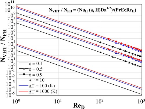
The dimensionless LEG term in Equation (58) shows five key factors which define the magnitude of each entropy generation mechanism. Figure 3 shows the variation of the two most significant parameters, comparing their development under different porosities, temperatures, and ranging the porous Reynolds number from 10 to 1000.

Figure 3. Heat transfer dimensionless factors, from laminar to turbulent porous Reynolds regimes.

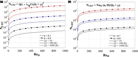
As shown in Figure 3, the heat transfer dimensionless factors were analyzed ranging the inlet temperature difference ΔT from 10 to 1000 K. The heat conduction factor $N_{\text{CHT}}$ and the volumetric heat transfer factor $N_{\text{VHT}}$ reach their highest values about 3 and 6 magnitude orders, respectively, when the Reynolds number is over 200; and reaches its maximum value for $\varphi =0.9$ at ΔT = 1000 K. As expected, the volumetric heat transfer dominates the heat transfer LEG and reaches its maximum value for higher porosities, which it is translated as higher exchange areas. Nevertheless, a CFD analysis is necessary to conclude the influence of each mechanism and to determine its spatial distribution, because the two phenomena obey to different temperature fields. The conduction obeys the fluid field temperature and the volumetric heat transfer to the interaction phenomenon between the two phases.

Analogously, Figure 4 shows the same dimensionless analysis applied to the viscous and hydrodynamic mechanisms of LEG. Due to the low viscosity that the working fluid (air) exhibits in the complete range of analysis, the viscous LEG is negligible for all cases. The same effect occurs for Darcy’s viscous hydrodynamic resistance, which is negligible for the complete domain analyzed. On the other hand, Forchheimer’s hydrodynamic resistance does present a significant impact on the LEG. The value of $N_{\text{FH}}$ reaches 9 magnitude orders for porosity of 0.1. In low porosities configurations, the fluid is constantly impinging on the solid matrix, significantly increasing the amount of useless work done by the flow over the porous media.

Figure 4. Viscous dissipation, Darcy’s, and Forchheimer’s hydrodynamic resistances dimensionless factors, from laminar to turbulent porous Reynolds regimes.

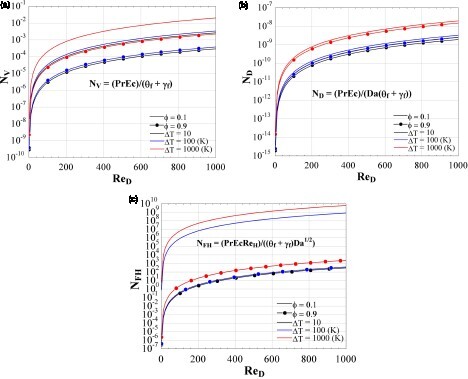
Summarizing the dimensionless analysis of each LEG mechanism in Figures 3 and 4, the maximum values of each magnitude factor are: $N_{\text{CHT}}$ < 2 × 10³, $N_{\text{VHT}}$ < 2 × 10⁶, $N_V$ < 10⁻¹, $N_D$ < 10⁻⁷, $N_{\text{FH}}$ < 10¹⁰.

Usually, the hydrodynamic effects are neglected in entropy generation analyses (Bejan, 1995). Nevertheless, the magnitude of the Forchheimer’s hydrodynamic term expressed through $N_{\text{FH}}$, makes necessary to consider its effect in differential CFD analyses, in either laminar or turbulent regimes. Figure 5 shows the distribution of $N_{\text{VHT}}/N_{\text{FH}}$ to compare the impact of each LEG mechanism on the different ranges of analysis (porosity, temperature difference, and porous Reynolds regime).

Figure 5. Comparison of dimensionless volumetric heat transfer against the Forchheimer’s hydrodynamic resistance effect over the LEG.

From Figure 5 it is possible to recognize the inflection points where the Forchheimer’s hydrodynamic resistance dominates the LEG in comparison to the volumetric heat transfer. For a porosity of 0.1, the magnitude of $N_{\text{FH}}$ dominates from $\text{R}{\text{e}}_D$ of 13.43, 29.92, and 36.62, for ΔT of 10, 100, and 1000 K, respectively. For higher porosities, 0.5 and 0.9, the volumetric heat transfer phenomenon dominates the LEG rate but is necessary a numerical CFD analysis to define with accuracy the regions in the domain where each mechanism dominates the others.

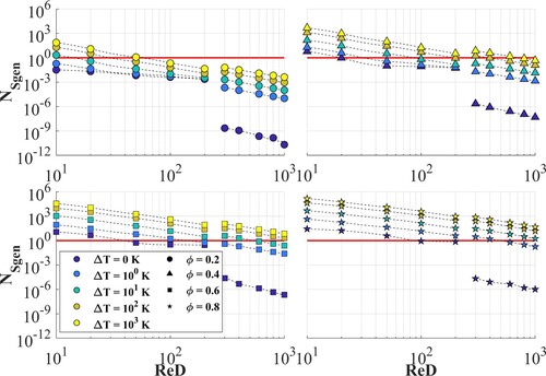
Consequently, a CFD analysis was conducted to adjust the preliminary results in Figure 5. Figure 6 shows the computational results for a parametrical analysis under different boundary conditions and operation configurations, ranging the porosity of the solid matrix from 0.2 to 0.8, and the solid-fluid inlet temperature difference from 0 to 1000 K. These results could be useful for low temperature configurations as sensible thermal energy storages, and for high-temperature differences as VSR. $N_{\text{Sgen}}$ compares the integrated LEG on the entire volume of heat transfer against the viscous and hydrodynamic resistances. As was appreciated in the previous dimensionless analysis, the Forchheimer’s effects are more relevant under higher porous Reynolds regimes, and its influence decreases with porosity. Considering the cases of ΔT below 100 K, the viscous and hydrodynamic resistances are dominant from $\text{R}{\text{e}}_D$ of 20, 100, 600, and 1000 for porosities of 0.2, 0.4, 0.6, and 0.8, respectively. These ranges of ΔT are commonly observed in sensible TES, where the temperature differences between solid and fluid phases are under 100 K, for charge and discharge cycles. Therefore, it is recommended to consider Forchheimer’s effects in LEG analysis. Analogously, ΔT ranges from 100 K show the dominance of the heat transfer LEG mechanisms under laminar and turbulent regimes for porosities higher than 0.6. These configurations are usually observed on VSR systems where the porosities are around 0.8 and the temperature differences on the inlet are close to 1000 K.

Figure 6. Comparison factor for the volumetric heat transfer against the Forchheimer’s hydrodynamic resistance effect over the LEG.

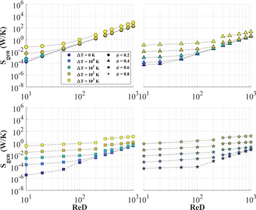
Finally, Figure 7 shows the total entropy generation rate for the aforementioned range of porosity, solid-fluid inlet temperature difference, and the Reynolds flow regime. The entropy rate reaches its maximum value of 825.18 W/K for a porosity of 0.2, regardless of the temperature difference. This is due to the high impact of the hydrodynamic resistance on the LEG rate, presented in Figure 6. On the other hand, for porosities higher than 0.6 the total entropy generation rate does not show significant variation, where the higher influence is assumed by the inlet solid-fluid temperature difference.

Figure 7. Entropy generation rate integrated for the complete volume.

5. Conclusions

A detailed physical and mathematical procedure was proposed to determine the entropy transport equation for fluid flow in a porous medium, from laminar to turbulent regimes. The entropy transport equation was developed using the Reynolds’ time-averaging method and the spatial volume-averaging method. In addition, a methodology to determine the LEG from the formulated thermophysical local entropy transport model (Equation (31)), was developed as a post-process function from the velocity, temperature, k, and ϵ fields, commonly resulting from regular CFD analysis. The proposed methodology allows determining the LEG without solving an additional transport entropy equation. The LEG model allows studying the performance of a porous heat exchange device, distinguishing different LEG mechanisms (or irreversibility sources), such as momentum dissipation phenomena, porous hydraulic resistance and heat transfer effects, in a single figure of merit. Thus, it is possible to measure the disadvantages related to the pressure drop and viscous effects of a porous media (${〈{\dot{s}}_{\mathrm{\Phi }}〉}^v$), and at the same time, determine the benefits related to the large heat exchanging area related to the porous matrix. In addition, through the entropy concept, the most rational way to exchange thermal energy is recognized, distinguishing the level of irreversibility (${〈{\dot{s}}_{\mathrm{\Theta }}〉}^v$) of each design configuration.

A numerical experiment was developed to study and compare the dominance of the different LEG mechanisms, considering different configurations of inlet temperature, porosity, and flow regime. The results are proposed as a starting point for future CFD entropy analysis applied to solar thermal sensible heat storage systems, solar hydrogen generation reactors, and volumetric solar receivers.

From the numerical results, the hydrodynamic resistance predominates on heat transfer effects over the total LEG for porosities under 0.4 at temperature differences below 100 K. Therefore, it is recommended to include hydrodynamic resistance in the LEG analysis of sensible TES. Analogously, the heat transfer LEG could be about 10³ times the magnitude of viscous and hydrodynamic dissipation effects, for porosities larger than 0.6, and at temperature differences from 100 and larger. Thus, high-temperature VSR analyses should include heat transfer effects in LEG analysis to ensure the accuracy of its results.

An analysis based on a LEG model allows to recognize and compare the impact of all the irreversibility mechanisms in a single figure of merit, allowing to define the main focuses in the optimization procedure, during the design of porous media systems. In future research, the proposed LEG expression and the dimensionless parameters could be implemented to study more working fluids and porous media configurations (wire mesh, wool, packed bed, ceramic foam, etc.), allowing to optimize novel applications on storage, exchange and generate energy, and/or energy conversion systems at differential scales.

Nomenclature

Table

$a_i$	solid-fluid surface area per unit of volume
$c_E$	Ergun’s inertia coefficient
$c_p$	specific heat at constant pressure
$\text{Da}$	Darcy number, $\text{Da}={\displaystyle \frac{K}{{d_p}^2}}$
$d_p$	mean pore diameter
e	internal energy per unit of mass
$Ec$	Eckert number, $Ec={\displaystyle \frac{{U_0}^2}{c_{p,f}\left(T_w-T_{f,\text{in}}\right)}}$
$f_j$	mass forces vector
$G_i$	generation rate of ${k_t}^i$
$H$	channel height
$h_i$	interfacial convective heat transfer
$k$	turbulent kinetic energy (TKE)
$K$	permeability of the porous media
$k_{\mathrm{\Theta }}$	variance of the temperature time-fluctuation
$N_{\text{CHT}}$	dimensionless LEG regarded to conductive heat transfer
$N_D$	dimensionless LEG due to Darcy hydrodynamic resistance
$N_{\text{FH}}$	dimensionless LEG due to Forchheimer hydrodynamic resistance
$\text{N}{\text{u}}_H$	Nusselt number, $\text{N}{\text{u}}_H={\displaystyle \frac{h_{i}H}{{\lambda }_f}}$
$N_{\text{Sgen}}$	entropy generation comparison dimensionless factor, $N_{\text{Sgen}}={\displaystyle \frac{{\dot{s}}_{\mathrm{\Phi }}}{{\dot{s}}_{\mathrm{\Theta }}}}$
$N_V$	dimensionless LEG regarded to Forchheimer hydrodynamic resistance
$N_{\text{VHT}}$	dimensionless LEG due to Forchheimer hydrodynamic resistance
$L$	channel length
$P$	pressure
$\text{Pr}$	Prandtl number, $\text{Pr}={\displaystyle \frac{\mu C_{p,f}}{{\lambda }_f}}$
$\text{P}{\text{r}}_t$	turbulent Prandtl number, $\text{P}{\text{r}}_t={\displaystyle \frac{{\mu }_t}{{\alpha }_t}}$
$\text{P}{\text{r}}_{t\varphi }$	turbulent volume-average Prandtl number, $\text{P}{\text{r}}_{t\varphi }={\displaystyle \frac{{\mu }_{t\varphi }}{{\alpha }_{t\varphi }}}$
$P_i$	production rate of ${〈k_t〉}^i$
$P_{k,\mathrm{\Theta }}$	production rate of $k_{\mathrm{\Theta }}$
$q_j$	net the heat flux
$R$	hydrodynamic drag force of the porous media
$\text{R}{\text{e}}_D$	Reynolds number based in $d_p$ and $u_D$, $\text{R}{\text{e}}_D={\displaystyle \frac{\rho u_D{d}_p}{\mu }}$
$\text{R}{\text{e}}_H$	Reynolds number based in $H$ and $u_D$, $\text{R}{\text{e}}_H={\displaystyle \frac{\rho u_{D}H}{\mu }}$
$s$	specific entropy
${〈{\dot{s}}_{\text{gen}}〉}^v$	total entropy generation rate
${〈{\dot{s}}_{\mathrm{\Phi }}〉}^v$	LEG rate due to hydrodynamic and viscous effects
${〈{\dot{s}}_{\mathrm{\Theta }}〉}^v$	LEG rate regarded to heat transfer
${〈{\dot{s}}_{\mathrm{\Theta },\overline{C}}〉}^v$	LEG rate by the conductive heat transfer related to the time-average fluid temperature
${〈{\dot{s}}_{\mathrm{\Theta },C^{\mathrm{\prime }}}〉}^v$	LEG rate due to the conductive heat transfer associated to the fluid temperature time-fluctuations
${〈{\dot{s}}_{\mathrm{\Phi },\overline{D}}〉}^v$	LEG rate due to viscous dissipation related to the time-average velocity
${〈{\dot{s}}_{\mathrm{\Phi },D^{\mathrm{\prime }}}〉}^v$	LEG rate by viscous dissipation regarded to the fluid velocity time-fluctuations
${\dot{s}}_{\mathrm{\Phi },DF}$	LEG rate associated to the Darcy–Forchheimer’s hydrodynamic resistance
${\dot{s}}_{\mathrm{\Theta },V}$	LEG rate regarded to the volumetric heat transfer between the solid and fluid phases
$T$	temperature
$u$	fluid velocity
$u_D$	Darcy’s velocity
$U_0$	fluid velocity at the inlet
$C_{\mu }$, $C_{1ϵ}$, $C_{2ϵ}$, ${\sigma }_k$, ${\sigma }_{ϵ}$	coefficients for $k$−$ϵ$ turbulence model
$k_1,k_2$	Darcy and Forchheimer hydrodynamic resistance parameters
Greek symbols
$\alpha$	thermal diffusivity
${\alpha }_t$	turbulent thermal diffusivity
${\alpha }_{t\varphi }$	macroscopic turbulent thermal diffusivity
$\gamma$	dimensionless inlet temperature, $\gamma ={\displaystyle \frac{T_{\text{in}}}{T_w-T_{\text{in}}}}$
$ϵ$	dissipation rate of TKE
${ϵ}_{\mathrm{\Theta }}$	dissipation rate of $k_{\mathrm{\Theta }}$
$\theta$	dimensionless temperature difference, $\theta ={\displaystyle \frac{T_w-T}{T_w-T_{\text{in}}}}$
$\lambda$	thermal conductivity
${\lambda }_{fs}$	local thermal conductivity tensor
${\lambda }_{t\varphi }$	macroscopic turbulent thermal conductivity
$\mu$	viscosity
${\mu }_t$	turbulent viscosity
${\mu }_{t\varphi }$	macroscopic turbulent viscosity
$\rho$	density
$\sigma$	surface forces tensor
$\varphi$	porosity
$\mathrm{\Phi }$	viscous dissipation rate
Subscripts
f	fluid
in	inlet
out	outlet
s	solid
$w$	wall side
Special symbols
${〈\phi 〉}^v$	volume-average value of $\phi$
${〈\phi 〉}^i$	intrinsic volume-average value of $\phi$
${}^i\phi$	spatial-dispersion of $\phi$
$\overline{\phi }$	time-average value of $\phi$
${\phi }^{\mathrm{\prime }}$	time-fluctuation of $\phi$

Disclosure statement

No potential conflict of interest was reported by the author(s).

Additional information

Funding

The authors wish to express their gratitude for the financial support from the project ANID/FONDAP 15110019 ‘Solar Energy Research Center’ – SERC-Chile and the project Fondecyt N° 11140725 from Chilean ANID. In addition, C. Sarmiento-Laurel would like to acknowledge the PhD scholarship ANID PFCHA/Doctorado Nacional 2018/2018-21181794.

Appendix

Appendix 1

(A1) $\begin{array}{rl}& \frac{D}{Dt}\left({\rho }_{f}e+\frac{1}{2}{\rho }_f{u}_j{u}_j\right)=\frac{\mathrm{\partial }}{\mathrm{\partial }{x}_i}\left(u_j{\sigma }_{ij}\right)+u_j{\rho }_f{f}_i-\frac{\mathrm{\partial }{q}_j}{\mathrm{\partial }{x}_j}\end{array}$(A1) (A2) $\begin{array}{rl}& \frac{\mathrm{\partial }}{\mathrm{\partial }t}\left({\rho }_{f}e+\frac{1}{2}{\rho }_f{u}_j{u}_j\right)+\frac{\mathrm{\partial }}{\mathrm{\partial }{x}_k}\left[\left({\rho }_{f}e+\frac{1}{2}{\rho }_f{u}_j{u}_j\right)u_k\right]\\ & =\frac{\mathrm{\partial }}{\mathrm{\partial }{x}_i}\left(u_j{\sigma }_{ij}\right)+u_j{\rho }_f{f}_j-\frac{\mathrm{\partial }{q}_j}{\mathrm{\partial }{x}_j}\end{array}$(A2) where $e$ is internal energy per unit of mass, ${\sigma }_{ij}$ the surface forces tensor, $f_j$ the mass forces vector and $q_j$ net the heat flux.

Then, expanding and regrouping the left-hand side terms, (A3) $\begin{array}{rl}& \frac{\mathrm{\partial }}{\mathrm{\partial }t}\left({\rho }_{f}e+\frac{1}{2}{\rho }_f{u}_j{u}_j\right)+\frac{\mathrm{\partial }}{\mathrm{\partial }{x}_k}\left[\left({\rho }_{f}e+\frac{1}{2}{\rho }_f{u}_j{u}_j\right)u_k\right]\\ & =\frac{\mathrm{\partial }}{\mathrm{\partial }t}\left({\rho }_f\right)e+{\rho }_f\frac{\mathrm{\partial }}{\mathrm{\partial }t}\left(e\right)+\frac{\mathrm{\partial }}{\mathrm{\partial }t}\left({\rho }_f\right)\frac{1}{2}{u}_j{u}_j\\ & +{\rho }_f\frac{\mathrm{\partial }}{\mathrm{\partial }t}\left(\frac{1}{2}{u}_j{u}_j\right)+\frac{\mathrm{\partial }}{\mathrm{\partial }{x}_k}\left(e\right){\rho }_f{u}_k+e\frac{\mathrm{\partial }}{\mathrm{\partial }{x}_k}\left({\rho }_f{u}_k\right)\\ & +\frac{\mathrm{\partial }}{\mathrm{\partial }{x}_k}\left({\rho }_f{u}_k\right)\frac{1}{2}{u}_j{u}_j+\frac{\mathrm{\partial }}{\mathrm{\partial }{x}_k}\left(\frac{1}{2}{u}_j{u}_j\right){\rho }_f{u}_k\end{array}$(A3) (A4) $\begin{array}{rl}& =e\left(\frac{\mathrm{\partial }}{\mathrm{\partial }t}\left({\rho }_f\right)+\frac{\mathrm{\partial }}{\mathrm{\partial }{x}_k}\left({\rho }_f{u}_k\right)\right)+{\rho }_f\frac{\mathrm{\partial }}{\mathrm{\partial }t}\left(e\right)\\ & +\frac{1}{2}{u}_j{u}_j\left(\frac{\mathrm{\partial }}{\mathrm{\partial }t}\left({\rho }_f\right)+\frac{\mathrm{\partial }}{\mathrm{\partial }{x}_k}\left({\rho }_f{u}_k\right)\right)\\ & +{\rho }_f\frac{\mathrm{\partial }}{\mathrm{\partial }t}\left(\frac{1}{2}{u}_j{u}_j\right)+\frac{\mathrm{\partial }}{\mathrm{\partial }{x}_k}\left(e\right){\rho }_f{u}_k+\frac{\mathrm{\partial }}{\mathrm{\partial }{x}_k}\left(\frac{1}{2}{u}_j{u}_j\right){\rho }_f{u}_k\end{array}$(A4)

Substituting the continuity equation in the first and second parentheses in Equation (A4). (A5) $\begin{array}{rl}& e\left(\frac{\mathrm{\partial }}{\mathrm{\partial }t}\left({\rho }_f\right)+\frac{\mathrm{\partial }}{\mathrm{\partial }{x}_k}\left({\rho }_f{u}_k\right)\right)+{\rho }_f\frac{\mathrm{\partial }}{\mathrm{\partial }t}\left(e\right)\\ & +\frac{1}{2}{u}_j{u}_j\left(\frac{\mathrm{\partial }}{\mathrm{\partial }t}\left({\rho }_f\right)+\frac{\mathrm{\partial }}{\mathrm{\partial }{x}_k}\left({\rho }_f{u}_k\right)\right)\\ & +{\rho }_f\frac{\mathrm{\partial }}{\mathrm{\partial }t}\left(\frac{1}{2}{u}_j{u}_j\right)+\frac{\mathrm{\partial }}{\mathrm{\partial }{x}_k}\left(e\right){\rho }_f{u}_k+\frac{\mathrm{\partial }}{\mathrm{\partial }{x}_k}\left(\frac{1}{2}{u}_j{u}_j\right){\rho }_f{u}_k\\ & ={\rho }_f\frac{\mathrm{\partial }}{\mathrm{\partial }t}\left(e\right)+{\rho }_f\frac{\mathrm{\partial }}{\mathrm{\partial }t}\left(\frac{1}{2}{u}_j{u}_j\right)+\frac{\mathrm{\partial }}{\mathrm{\partial }{x}_k}\left(e\right){\rho }_f{u}_k\\ & +\frac{\mathrm{\partial }}{\mathrm{\partial }{x}_k}\left(\frac{1}{2}{u}_j{u}_j\right){\rho }_f{u}_k\end{array}$(A5) (A6) $\begin{array}{rl}& ={\rho }_f\frac{\mathrm{\partial }}{\mathrm{\partial }t}\left(e\right)+\frac{\mathrm{\partial }}{\mathrm{\partial }{x}_k}\left(e\right){\rho }_f{u}_k+{\rho }_f{u}_j\frac{\mathrm{\partial }}{\mathrm{\partial }t}\left(u_j\right)+\frac{\mathrm{\partial }}{\mathrm{\partial }{x}_k}\left(u_j\right){\rho }_f{u}_j{u}_k\end{array}$(A6)

Thus, including Equation (A6) in Equation (A1), (A7) $\begin{array}{rl}& {\rho }_f\left[\left(\frac{\mathrm{\partial }}{\mathrm{\partial }t}\left(e\right)+\frac{\mathrm{\partial }}{\mathrm{\partial }{x}_k}\left(e\right)u_k\right)+\left(u_j\frac{\mathrm{\partial }}{\mathrm{\partial }t}\left(u_j\right)+\frac{\mathrm{\partial }}{\mathrm{\partial }{x}_k}\left(u_j\right)u_j{u}_k\right)\right]\\ & =u_j\frac{\mathrm{\partial }}{\mathrm{\partial }{x}_i}\left({\sigma }_{ij}\right)+{\sigma }_{ij}\frac{\mathrm{\partial }}{\mathrm{\partial }{x}_i}\left(u_j\right)+u_j{\rho }_f{f}_j-\frac{\mathrm{\partial }{q}_j}{\mathrm{\partial }{x}_j}\end{array}$(A7)

Appendix 2

Volume-averaging method

In a similar form to the time-average proposed by Reynolds in 1895 (Reynolds et al., 1895), the macroscopic analysis considers a REV as the minimum volume of analysis of Slattery (de Lemos, 2012; Slattery, 1967). For a fluid property $\phi$, the volumetric average over a REV is as follows. (A8) ${〈\phi 〉}^V=\frac{1}{\Delta V}{\int }_{\Delta V}\phi dV$(A8) where ${〈\phi 〉}^V$ is the average value of $\phi$ at any point inside of a REV of size $\Delta V$. Then, the value of ${〈\phi 〉}^V$ is related to the intrinsic average for the fluid phase ${〈{\phi }_f〉}^i$ as follows. (A9) ${〈{\phi }_f〉}^V=\varphi {〈{\phi }_f〉}^i$(A9) where $\varphi$ is the porosity.

Then, in the same way of the Reynolds times averaging methodology, the property $\phi$ can be separated in its volume-averaged expression ${〈\phi 〉}^i$ and its spatial deviation ${}^i\phi$, as follows (de Lemos, 2012; Hsu & Cheng, 1990; Quintard & Whitaker, 1994). (A10) $\phi ={〈\phi 〉}^i+{}^i\phi$(A10)

In addition, for deriving operators Slattery (Slattery, 1967) presents the following relationship to consider the flow of a property between phases, as heat or surface forces. (A11) $\begin{array}{rl}{〈\frac{\mathrm{\partial }}{\mathrm{\partial }{x}_i}\left(\phi \right)〉}^V& =\frac{\mathrm{\partial }}{\mathrm{\partial }{x}_i}\left(\varphi {〈\phi 〉}^i\right)+\frac{1}{\Delta V}{\int }_{A_i}\mathit{n}\phi d{s}_i\end{array}$(A11) (A12) $\begin{array}{rl}{〈\frac{\mathrm{\partial }{\phi }_k}{\mathrm{\partial }{x}_k}〉}^V& =\frac{\mathrm{\partial }}{\mathrm{\partial }{x}_k}\left(\varphi {〈{\phi }_k〉}^i\right)+\frac{1}{\Delta V}{\int }_{A_i}\mathit{n}\cdot \phi d{s}_i\end{array}$(A12) where $n$ is the unitary normal vector, and $u_i$ the velocity phase to the interfacial area $A_i$ between the fluid and solid phases.

Time-average and spatial-average

To take into account the turbulent effects in porous media de Lemos proposes a double decomposition in space and time as follows (de Lemos, 2012). (A13) $\phi =〈\overline{\phi }+{\phi }^{\mathrm{\prime }}{〉}^i+{}^i\left(\overline{\phi }+{\phi }^{\mathrm{\prime }}\right)$(A13) then, (A14) $\phi =〈\overline{\phi }{〉}^i+〈{\phi }^{\mathrm{\prime }}{〉}^i+{}^i\overline{\phi }+{}^i{\phi }^{\mathrm{\prime }}$(A14) where $〈\overline{\phi }{〉}^i$ is the time and volume-averaged $\phi$, $〈{\phi }^{\mathrm{\prime }}{〉}^i$ is the volume-average of the time-fluctuation of $\phi$, ${}^i\overline{\phi }$ is the volume deviation of the time-average of $\phi$ and ${}^i{\phi }^{\mathrm{\prime }}$ is the volume-deviation of the time-fluctuation of $\phi$.

Appendix 3

Multiplying for $u_j$ and applying the spatial-averaging method over the momentum transport equation, the relation used in Equation (11) is determined as follows: (A15) $\begin{array}{rl}& {\rho }_f\frac{\mathrm{\partial }}{\mathrm{\partial }t}\left(u_j\right)+{\rho }_f{u}_k\frac{\mathrm{\partial }}{\mathrm{\partial }{x}_k}\left(u_j\right)=\frac{\mathrm{\partial }}{\mathrm{\partial }{x}_i}\left({\sigma }_{ij}\right)+{\rho }_f{f}_i\end{array}$(A15) (A16) $\begin{array}{rl}& \varphi {〈u_j\left[{\rho }_f\frac{\mathrm{\partial }}{\mathrm{\partial }t}\left(u_j\right)+{\rho }_f{u}_k\frac{\mathrm{\partial }}{\mathrm{\partial }{x}_k}\left(u_j\right)\right]〉}^i=\varphi {〈u_j\left[\frac{\mathrm{\partial }}{\mathrm{\partial }{x}_i}\left({\sigma }_{ij}\right)+{\rho }_f{f}_i\right]〉}^i\end{array}$(A16) (A17) $\begin{array}{rl}& \varphi {〈{\rho }_f{u}_j\frac{\mathrm{\partial }}{\mathrm{\partial }t}\left(u_j\right)+{\rho }_f{u}_j{u}_k\frac{\mathrm{\partial }}{\mathrm{\partial }{x}_k}\left(u_j\right)〉}^i=\varphi {〈u_j\frac{\mathrm{\partial }}{\mathrm{\partial }{x}_i}\left({\sigma }_{ij}\right)+{\rho }_f{u}_j{f}_i〉}^i\end{array}$(A17) (A18) $\begin{array}{rl}& {\rho }_f\varphi {〈u_j\frac{\mathrm{\partial }}{\mathrm{\partial }t}\left(u_j\right)〉}^i+{\rho }_f\varphi {〈u_j{u}_k\frac{\mathrm{\partial }}{\mathrm{\partial }{x}_k}\left(u_j\right)〉}^i\\ & =\varphi {〈u_j\frac{\mathrm{\partial }}{\mathrm{\partial }{x}_i}\left({\sigma }_{ij}\right)〉}^i+\varphi ({〈u_j〉}^i{〈\frac{\mathrm{\partial }}{\mathrm{\partial }{x}_i}\left({\sigma }_{ij}\right)〉}^i\\ & +{〈{}^i\left(u_j\right){\$}^i\$\left(\frac{\mathrm{\partial }}{\mathrm{\partial }{x}_i}\left({\sigma }_{ij}\right)\right)〉}^i)+\varphi {〈{\rho }_f{u}_j{f}_i〉}^i\end{array}$(A18)

Appendix 4

From the Gibbs equation (Cantwell, 2018). (A19) $\begin{array}{rl}T\frac{Ds}{Dt}& =\frac{De}{Dt}+P\frac{D\left(1/\rho \right)}{Dt}\end{array}$(A19) (A20) $\begin{array}{rl}T\frac{Ds}{Dt}& =\frac{De}{Dt}-\frac{P}{{\rho }^2}\frac{D\rho }{Dt}\end{array}$(A20) (A21) $\begin{array}{rl}\rho T\frac{Ds}{Dt}& =\rho \frac{De}{Dt}-\frac{P}{\rho }\frac{D\rho }{Dt}\end{array}$(A21)

Appendix 5

Continuity and momentum equations

(A22) $\begin{array}{rl}& \frac{\mathrm{\partial }{\rho }_f}{\mathrm{\partial }t}+{\rho }_f\frac{\mathrm{\partial }}{\mathrm{\partial }{x}_k}\left({\varphi 〈{\overline{u}}_k〉}^i\right)=0\end{array}$(A22) (A23) $\begin{array}{rl}& \frac{\mathrm{\partial }\left({\rho }_f\varphi {〈\overline{u}〉}^i\right)}{\mathrm{\partial }t}+{\rho }_f\frac{\mathrm{\partial }}{\mathrm{\partial }{x}_k}\left(\varphi {〈{\overline{u}}_j{\overline{u}}_k〉}^i\right)\\ & =\frac{\mathrm{\partial }}{\mathrm{\partial }{x}_i}(-\varphi {〈\overline{P}〉}^i{\delta }_{ij}+\varphi \mu \left(\frac{\mathrm{\partial }{〈\overline{u_i}〉}^i}{\mathrm{\partial }{x}_j}+\frac{\mathrm{\partial }{〈\overline{u_j}〉}^i}{\mathrm{\partial }{x}_i}\right)\\ & -\frac{2}{3}\varphi \mu \left({\delta }_{ij}\frac{\mathrm{\partial }{〈\overline{u_k}〉}^i}{\mathrm{\partial }{x}_k}\right)\phantom{\left(\frac{\mathrm{\partial }{〈u_i〉}^i}{\mathrm{\partial }{x}_j}+\frac{\mathrm{\partial }{〈u_j〉}^i}{\mathrm{\partial }{x}_i}\right)})\\ & -{\rho }_f\frac{\mathrm{\partial }}{\mathrm{\partial }{x}_k}\left(\varphi \overline{{〈{u_j}^{\mathrm{\prime }}{u_k}^{\mathrm{\prime }}〉}^i}\right)-\varphi \left(\frac{{\mu }_f}{k_1}\overline{u_D}+\frac{{\rho }_f}{k_2}|\overline{u_D}|\overline{u_D}\right)\end{array}$(A23) where ${\rho }_f$ is the fluid density, $\overline{u}$ the time-averaged velocity, $u^{\mathrm{\prime }}$ the velocity time-fluctuation term, $\varphi$ the porosity, $\overline{P}$ the time-averaged fluid’s pressure and $\mu$ fluid’s viscosity.

The last two terms derive from the expressions (3) and (4) applied to both surface force terms, pressure, and viscous shear stress. They represent the interaction between the fluid with the solid matrix as a drag force. Commonly are defined as Darcy–Forchheimer terms (Pedras & De Lemos, 2001), as follows: (A24) $\overline{R}=\varphi \left(\frac{{\mu }_f}{k_1}\overline{u_D}+\frac{{\rho }_f}{k_2}|\overline{u_D}|\overline{u_D}\right)$(A24)

The last two in (10) are determined experimentally, considering the Darcian velocity $u_D=\varphi {〈\overline{u}〉}^i$, where $k_1$ and $k_2$ are correlation constants.

Energy equation

The energy equation is split into two parts to consider NTE (de Lemos, 2012) between both phases (fluid and solid). (A25) $\begin{array}{rl}& {\rho }_f{c}_{p,f}\left(\frac{\mathrm{\partial }\left(\varphi {〈\overline{T_f}〉}^i\right)}{\mathrm{\partial }t}+\frac{\mathrm{\partial }}{\mathrm{\partial }{x}_k}\left(\varphi {〈\overline{T_f}{\overline{u}}_k〉}^i\right)\right)\\ & =\frac{\mathrm{\partial }}{\mathrm{\partial }{x}_k}\left(\varphi {\lambda }_f\frac{\mathrm{\partial }{〈\overline{T_f}〉}^i}{\mathrm{\partial }{x}_k}\right)-{\rho }_f{c}_{p,f}\frac{\mathrm{\partial }}{\mathrm{\partial }{x}_k}\left(\varphi \overline{{〈{T_f}^{\mathrm{\prime }}{u^{\mathrm{\prime }}}_k〉}^i}\right)\\ & +h_i{a}_i\left({〈\overline{T_s}〉}^i-{〈\overline{T_f}〉}^i\right)\end{array}$(A25) (A26) $\begin{array}{rl}& {\rho }_s{c}_{p,s}\frac{\mathrm{\partial }\left(\left(1-\varphi \right){〈\overline{T_s}〉}^i\right)}{\mathrm{\partial }t}\\ & =\frac{\mathrm{\partial }}{\mathrm{\partial }{x}_k}\left(\left(1-\varphi \right){\lambda }_s\frac{\mathrm{\partial }{〈\overline{T_f}〉}^i}{\mathrm{\partial }{x}_k}\right)-h_i{a}_i\left({〈\overline{T_s}〉}^i-{〈\overline{T_f}〉}^i\right)\ast 6pt\end{array}$(A26) where $c_p$ is the specific heat, $\lambda$ the thermal conductivity, $\overline{T}$ is time-averaged temperature, $T^{\mathrm{\prime }}$ the temperature fluctuation in time term, and the subscripts $f$ and $s$ are related to fluid and solid phases, respectively.

References

- Alazmi, B., & Vafai, K. (2000). Analysis of variants within the porous media transport models. Journal of Heat Transfer, 122(2), 303–326. https://doi.org/10.1115/1.521468
- Avila-Marin, A. L. (2011). Volumetric receivers in solar thermal power plants with central receiver system technology: A review. Solar Energy, 85(5), 891–910. https://doi.org/10.1016/j.solener.2011.02.002
- Avila-marin, A. L., Caliot, C., Alvarez De Lara, M., Fernandez-Reche, J., Montes, M. J., & Martinez-tarifa, A. (2018). Homogeneous equivalent model coupled with P1-approximation for dense wire meshes volumetric air receivers. Renewable Energy, 135(2019), 908–919. https://doi.org/10.1016/j.renene.2018.12.061
- Avila-marin, A. L., Caliot, C., Flamant, G., Alvarez De Lara, M., & Fernandez-Reche, J. (2018). Numerical determination of the heat transfer coefficient for volumetric air receivers with wire meshes. Solar Energy, 162(December 2017), 317–329. https://doi.org/10.1016/j.solener.2018.01.034
- Avila-Marin, A. L., Fernandez-reche, J., & Martinez-tarifa, A. (2019). Modelling strategies for porous structures as solar receivers in central receiver systems: A review. Renewable and Sustainable Energy Reviews, 111(November 2018), 15–33. https://doi.org/10.1016/j.rser.2019.03.059
- Bai, F. (2010). One dimensional thermal analysis of silicon carbide ceramic foam used for solar air receiver. International Journal of Thermal Sciences, 49(12), 2400–2404. https://doi.org/10.1016/j.ijthermalsci.2010.08.010
- Baumann, A., Hoch, D., Behringer, J., & Niessner, J. (2020). Macro-scale modeling and simulation of two-phase flow in fibrous liquid aerosol filters. Engineering Applications of Computational Fluid Mechanics, 14(1), 1325–1336. https://doi.org/10.1080/19942060.2020.1828174
- Bejan, A. (1980). Second law analysis in heat transfer. Energy, 5(8–9), 720–732. https://doi.org/10.1016/0360-5442(80)90091-2
- Bejan, A. (1995). Entropy generation minimization (1st ed.). CRC Press.
- Bejan, A. (2013). Convection heat transfer (4th ed.). Hoboken, NJ: John Wiley & Sons Inc.
- Betchen, L. J., & Straatman, A. G. (2008). The development of a volume-averaged entropy-generation function for nonequilibrium heat transfer in high-conductivity porous foams. Numerical Heat Transfer, Part B: Fundamentals, 53(5), 412–436. https://doi.org/10.1080/10407790801960786
- Betchen, L. J., & Straatman, A. G. (2014). Entropy generation-based computational geometry optimization of the pore structure of high-conductivity graphite foams for use in enhanced heat transfer devices. Computers & Fluids, 103, 49–70. https://doi.org/10.1016/j.compfluid.2014.07.012
- Calderón-Vásquez, I., Cortés, E., García, J., Segovia, V., Caroca, A., Sarmiento, C., Barraza, R., & Cardemil, J. M. (2021). Review on modeling approaches for packed-bed thermal storage systems. Renewable and Sustainable Energy Reviews, 143(July 2021), 22. https://doi.org/10.1016/j.rser.2021.110902
- Cantwell, B. J. (2018). Fundamentals of compressible flow. In International Journal of Heat and Fluid Flow. Department of Aeronautics and Astronautics, Stanford University, California. https://doi.org/10.1016/0142-727x(83)90067-x
- Capuano, R., Fend, T., Schwarzbözl, P., Smirnova, O., Stadler, H., Hoffschmidt, B., & Pitz-Paal, R. (2016). Numerical models of advanced ceramic absorbers for volumetric solar receivers. Renewable and Sustainable Energy Reviews, 58, 656–665. https://doi.org/10.1016/j.rser.2015.12.068
- Currie, I. G. (2012). Fundamental mechanics of fluids (4th ed.). CRC Press.
- de Lemos, M. (2012). Turbulence in porous media modeling and applications (2nd ed.). Elsevier Academic Press.
- de Lemos, M., & Pedras, M. H. J. (2001). Recent mathematical models for turbulent flow in saturated rigid porous media. Journal of Fluids Engineering, 123(4), 935–940. https://doi.org/10.1115/1.1413243
- Ergun, S., & Orning, A. A. (1949). Fluid flow through randomly packed columns and fluidized beds. Industrial & Engineering Chemistry, 41(6), 1179–1184. https://doi.org/10.1021/ie50474a011
- Fend, T., Hoffschmidt, B., Pitz-Paal, R., Reutter, O., & Rietbrock, P. (2004). Porous materials as open volumetric solar receivers: Experimental determination of thermophysical and heat transfer properties. Energy, 29(5–6), 823–833. https://doi.org/10.1016/S0360-5442(03)00188-9
- Feng, Y., & Kleinstreuer, C. (2010). Nanofluid convective heat transfer in a parallel-disk system. International Journal of Heat and Mass Transfer, 53(21–22), 4619–4628. https://doi.org/10.1016/j.ijheatmasstransfer.2010.06.031
- Gersten, K., & Herwig, H. (1992). Strömungsmechanik. Vieweg.
- Ghalandari, M., Mirzadeh Koohshahi, E., Mohamadian, F., Shamshirband, S., & Chau, K. W. (2019). Numerical simulation of nanofluid flow inside a root canal. Engineering Applications of Computational Fluid Mechanics, 13(1), 254–264. https://doi.org/10.1080/19942060.2019.1578696
- Han, L., Lu, C., Yumashev, A., Bahrami, D., Kalbasi, R., Jahangiri, M., Karimipour, A., Band, S. S., Chau, K. W., & Mosavi, A. (2021). Numerical investigation of magnetic field on forced convection heat transfer and entropy generation in a microchannel with trapezoidal ribs. Engineering Applications of Computational Fluid Mechanics, 15(1), 1746–1760. https://doi.org/10.1080/19942060.2021.1984991
- Hischier, I., Leumann, P., & Steinfeld, A. (2012). Experimental and numerical analyses of a pressurized air receiver for solar-driven gas turbines. Journal of Solar Energy Engineering, 134(2), 1–8. https://doi.org/10.1115/1.4005446
- Ho, C. K. (2016). A review of high-temperature particle receivers for concentrating solar power. Applied Thermal Engineering, 109, 958–969. https://doi.org/10.1016/j.applthermaleng.2016.04.103
- Hsu, C. T., & Cheng, P. (1990). Thermal dispersion in a porous medium. International Journal of Heat and Mass Transfer, 33(8), 1587–1597. https://doi.org/10.1016/0017-9310(90)90015-M
- Kalita, J. C., & Dass, A. K. (2011). Higher order compact simulation of double-diffusive natural convection in a vertical porous annulus. Engineering Applications of Computational Fluid Mechanics, 5(3), 357–371. https://doi.org/10.1080/19942060.2011.11015378
- Kaviany, M. (1999). Principles of heat transfer in porous media. Springer. https://doi.org/10.1007/b22134
- Khan, F. A., & Straatman, A. G. (2016). Closure of a macroscopic turbulence and non-equilibrium turbulent heat and mass transfer model for a porous media comprised of randomly packed spheres. International Journal of Heat and Mass Transfer, 101, 1003–1015. https://doi.org/10.1016/j.ijheatmasstransfer.2016.05.106
- Kock, F., & Herwig, H. (2004). Local entropy production in turbulent shear flows: A high-Reynolds number model with wall functions. International Journal of Heat and Mass Transfer, 47(10–11), 2205–2215. https://doi.org/10.1016/j.ijheatmasstransfer.2003.11.025
- Kock, F., & Herwig, H. (2005). Entropy production calculation for turbulent shear flows and their implementation in cfd codes. International Journal of Heat and Fluid Flow, 26(4 SPEC. ISS.), 672–680. https://doi.org/10.1016/j.ijheatfluidflow.2005.03.005
- Kribus, A., Gray, Y., Grijnevich, M., Mittelman, G., Mey-Cloutier, S., & Caliot, C. (2014). The promise and challenge of solar volumetric absorbers. Solar Energy, 110, 463–481. https://doi.org/10.1016/j.solener.2014.09.035
- Kribus, A., Ries, H., & Spirkl, W. (1996). Inherent limitations of volumetric solar receivers. Journal of Solar Energy Engineering, 118(3), 151–155. https://doi.org/10.1115/1.2870891
- Kun-Can, Z., Tong, W., Hai-Cheng, L., Zhi-Jun, G., & Wen-Fei, W. (2017). Fractal analysis of flow resistance in random porous media based on the staggered pore-throat model. International Journal of Heat and Mass Transfer, 115, 225–231. https://doi.org/10.1016/j.ijheatmasstransfer.2017.07.031
- Kuwahara, F., Nakayama, A., & Koyama, H. (1996). A numerical study of thermal dispersion in porous media. Journal of Heat Transfer, 118(3), 756–761. https://doi.org/10.1115/1.2822696
- Lee, K., & Howell, J. R. (1987, March 22–27). Forced convective and radiative transfer within a highly porous layer exposed to a turbulent external flow field. Proceedings of the 1987 ASME-JSME. Thermal engineering joint conference, Honolulu, Vol. 2 (pp. 377–386).
- Liu, G., Gong, W., Wu, H., & Lin, A. (2021). Experimental and CFD analysis on the pressure ratio and entropy increment in a cover-plate pre-swirl system of gas turbine engine. Engineering Applications of Computational Fluid Mechanics, 15(1), 476–489. https://doi.org/10.1080/19942060.2021.1884600
- Mahian, O., Kianifar, A., Kleinstreuer, C., Al-Nimr, M. A., Pop, I., Sahin, A. Z., & Wongwises, S. (2013). A review of entropy generation in nanofluid flow. International Journal of Heat and Mass Transfer, 65, 514–532. https://doi.org/10.1016/j.ijheatmasstransfer.2013.06.010
- Moghaddami, M., Mohammadzade, A., & Esfehani, S. A. V. (2011). Second law analysis of nanofluid flow. Energy Conversion and Management, 52(2), 1397–1405. https://doi.org/10.1016/j.enconman.2010.10.002
- Nagano, Y., & Kim, C. (1988). A two-equation model for heat transport in wall turbulent shear flows. Journal of Heat Transfer, 110(3), 583–589. https://doi.org/10.1115/1.3250532
- Nakayama, A., & Kuwahara, F. (1999). A macroscopic turbulence model for flow in a porous medium. Journal of Fluids Engineering, 121(2), 427–433. https://doi.org/10.1115/1.2822227
- OpenFOAM v9. (2021). The OpenFOAM Foundation Ltd. https://openfoam.org/
- Pabst, C., Feckler, G., Schmitz, S., Smirnova, O., Capuano, R., Hirth, P., & Fend, T. (2017). Experimental performance of an advanced metal volumetric air receiver for solar towers. Renewable Energy, 106, 91–98. https://doi.org/10.1016/j.renene.2017.01.016
- Patankar, S. V. (1980). Numerical Heat Transfer and fluid flow (1st ed.). CRC Press. https://doi.org/10.1201/9781482234213
- Patankar, S. V. (1981). A calculation procedure for two-dimensional elliptic situations. Numerical Heat Transfer, 4(4), 409–425. https://doi.org/10.1080/01495728108961801
- Patankar, S. V., & Spalding, D. B. (1972). A calculation procedure for heat, mass and momentum transfer in three-dimensional parabolic flows. International Journal of Heat and Mass Transfer, 15(10), 1787–1806. https://doi.org/10.1016/0017-9310(72)90054-3
- Pedras, M. H. J., & De Lemos, M. (2001). Macroscopic turbulence modeling for incompressible flow through undeformable porous media. International Journal of Heat and Mass Transfer, 44(6), 1081–1093. https://doi.org/10.1016/S0017-9310(00)00202-7
- Quintard, M., & Whitaker, S. (1994). Transport in ordered and disordered porous media II: Generalized volume averaging. Transport in Porous Media, 14(2), 179–206. https://doi.org/10.1007/BF00615200
- Reynolds, O., M, A., L, D., & F, R. (1895). On the dynamical theory of incompressible viscous Fluids and the determination of the criterion. Philosophical Transactions of the Royal Society of London A, 10(186), 123–164. https://doi.org/10.1098/rsta.1895.0004
- Saito, M. B., & De Lemos, M. (2005). Interfacial heat transfer coefficient for non-equilibrium convective transport in porous media. International Communications in Heat and Mass Transfer, 32(5), 666–676. https://doi.org/10.1016/j.icheatmasstransfer.2004.06.013
- Salih, S. Q., Aldlemy, M. S., Rasani, M. R., Ariffin, A. K., Ya, T. M. Y. S. T., Al-Ansari, N., Yaseen, Z. M., & Chau, K. W. (2019). Thin and sharp edges bodies-fluid interaction simulation using cut-cell immersed boundary method. Engineering Applications of Computational Fluid Mechanics, 13(1), 860–877. https://doi.org/10.1080/19942060.2019.1652209
- Sarmiento, C., Cardemil, J. M., Calderón, W., & Herrmann, B. (2019, November 4–7). Heat transfer framework for selecting the structure of open volumetric air receivers. Proceedings ISES Solar World Congress 2019, Santiago, Chile. https://doi.org/10.18086/swc.2019.18.11
- Sciacovelli, A., Verda, V., & Sciubba, E. (2015). Entropy generation analysis as a design tool—A review. Renewable and Sustainable Energy Reviews, 43, 1167–1181. https://doi.org/10.1016/j.rser.2014.11.104
- Singh, S., Sørensen, K., Condra, T., Batz, S. S., & Kristensen, K. (2019). Investigation on transient performance of a large-scale packed-bed thermal energy storage. Applied Energy, 239(October 2018), 1114–1129. https://doi.org/10.1016/j.apenergy.2019.01.260
- Slattery, J. C. (1967). Flow of viscoelastic Fluids through porous media. AIChE Journal, 13(6), 1066–1071. https://doi.org/10.1002/aic.690130606
- Song, Z., & Liu, B. (2018). Optimization design for tandem cascades of compressors based on adaptive particle swarm optimization. Engineering Applications of Computational Fluid Mechanics, 12(1), 535–552. https://doi.org/10.1080/19942060.2018.1474806
- Spelling, J., Favrat, D., Martin, A., & Augsburger, G. (2012). Thermoeconomic optimization of a combined-cycle solar tower power plant. Energy, 41(1), 113–120. https://doi.org/10.1016/j.energy.2011.03.073
- Sutherland, W. (1893). LII. The viscosity of gases and molecular force. The London, Edinburgh, and Dublin Philosophical Magazine and Journal of Science, 36(223), 507–531. https://doi.org/10.1080/14786449308620508
- Teruel, F. E., & Rizwan-uddin. (2009a). A new turbulence model for porous media flows. Part I: Constitutive equations and model closure. International Journal of Heat and Mass Transfer, 52(19–20), 4264–4272. https://doi.org/10.1016/j.ijheatmasstransfer.2009.04.017
- Teruel, F. E., & Rizwan-uddin. (2009b). A new turbulence model for porous media flows. Part II: Analysis and validation using microscopic simulations. International Journal of Heat and Mass Transfer, 52(21–22), 5193–5203. https://doi.org/10.1016/j.ijheatmasstransfer.2009.04.023
- Ting, T. W., Hung, Y. M., & Guo, N. (2015). Entropy generation of viscous dissipative nanofluid flow in thermal non-equilibrium porous media embedded in microchannels. International Journal of Heat and Mass Transfer, 81, 862–877. https://doi.org/10.1016/j.ijheatmasstransfer.2014.11.006
- Torabi, M., Torabi, M., Eftekhari, M., & Peterson, G. P. (2019). Fluid flow, heat transfer and entropy generation analyses of turbulent forced convection through isotropic porous media using RANS models. International Journal of Heat and Mass Transfer, 132, 443–461. https://doi.org/10.1016/j.ijheatmasstransfer.2018.12.020
- Torabi, M., Torabi, M., & Peterson, G. P. (2017). Heat transfer and entropy generation analyses of forced convection through porous media using pore scale modeling. Journal of Heat Transfer, 139(1), 1–10. https://doi.org/10.1115/1.4034181
- Vafai, K. (2015). Handbook of porous media. In CRC (Ed.), Transport in porous media (Vol. 93, Issue 3). https://doi.org/10.1007/s11242-012-9985-0
- Villafán-Vidales, H. I., Abanades, S., Caliot, C., & Romero-Paredes, H. (2011). Heat transfer simulation in a thermochemical solar reactor based on a volumetric porous receiver. Applied Thermal Engineering, 31(16), 3377–3386. https://doi.org/10.1016/j.applthermaleng.2011.06.022
- Wilcox, D. C. (2006). Turbulence modeling for CFD. DCW Industries.
- Wu, J., & Yu, B. (2007). A fractal resistance model for flow through porous media. International Journal of Heat and Mass Transfer, 50(19–20), 3925–3932. https://doi.org/10.1016/j.ijheatmasstransfer.2007.02.009
- Wu, Z., Caliot, C., Bai, F., Flamant, G., Wang, Z., Zhang, J., & Tian, C. (2010). Experimental and numerical studies of the pressure drop in ceramic foams for volumetric solar receiver applications. Applied Energy, 87(2), 504–513. https://doi.org/10.1016/j.apenergy.2009.08.009
- Wu, Z., Caliot, C., Flamant, G., & Wang, Z. (2011). Coupled radiation and flow modeling in ceramic foam volumetric solar air receivers. Solar Energy, 85(9), 2374–2385. https://doi.org/10.1016/j.solener.2011.06.030
- Xu, C., Song, Z., Chen, L. d., & Zhen, Y. (2011). Numerical investigation on porous media heat transfer in a solar tower receiver. Renewable Energy, 36(3), 1138–1144. https://doi.org/10.1016/j.renene.2010.09.017
- Younis, L. B., & Viskanta, R. (1993). Experimental determination of the volumetric heat transfer coefficient between stream of air and ceramic foam. International Journal of Heat and Mass Transfer, 36(6), 1425–1434. https://doi.org/10.1016/S0017-9310(05)80053-5
Appendix
Appendix 1
(A1)
(A2)
(A2) where
is internal energy per unit of mass,
the surface forces tensor,
the mass forces vector and
net the heat flux.