Aerodynamic noise prediction of a high-speed centrifugal fan considering impeller-eccentric effect

ABSTRACT

In this paper, the aerodynamic noise of a centrifugal fan with an eccentric impeller is investigated and analyzed by adopting a hybrid method combining detached-eddy simulation and the acoustic finite element method (FEM). The impeller-eccentric effect of high-speed centrifugal fans, frequently ignored in theoretical studies, is objective in practical engineering applications owing to machining and installation errors, which have a significant influence on flow characteristics and subsequently noise characteristics. An impeller-whirling model combined with the sliding mesh method is introduced to obtain the actual flow with an eccentric impeller. First, the internal flow field handled with different eccentricities is investigated. The total pressure and internal efficiency decline, and the flow field near the leading edge shows intense unsteadiness, inducing a rise in the pressure fluctuation amplitude at the rotating frequency (RF) in both impeller flow passage and volute domain. Second, the variational formulation of Lighthill’s analogy is implemented by acoustic FEM to better account for the interaction between the solid surface and aerodynamic sound, capturing a contribution by turbulence noise at the second RF. Under eccentric conditions, the sound source intensity shows a circumferential non-uniform distribution in a similar region to the flow field. The calculated sound pressure level captures the variation in the experimental result, which shows an obvious rise at RF induced by the impeller-eccentric effect. The characteristics of the noise spectrum and sound directivity change significantly, and the overall sound pressure level rises with the increase in eccentricity. This study provides an effective simulation strategy for predicting the aerodynamic noise of centrifugal fans under realistic conditions.

KEYWORDS:

• Centrifugal fan
• eccentric impeller
• aerodynamic noise
• acoustic FEM

1. Introduction

High-speed centrifugal fans are widely applied in industry and civil engineering for ventilation (Shen et al., 2019), cooling (Krain, 2005) and numerous other uses (Burgmann et al., 2017) owing to their ability to generate high pressure, usually the core part in a system. However, their noise problems not only increase the environmental pollution, but also lead to awful working conditions for operators. When handling ideal impellers, the noise characteristics have been investigated extensively. Holste and Neise (1993) conducted experimental research on the acoustic characteristics of a centrifugal fan. Their results showed that the blade passing frequency (BPF) governs the frequency spectrum at the design speed, and the flow separation in the impeller domain contributes to the broadband noise. Kameier and Neise (1997) found that rotation instability was a necessary condition for the generation of tip clearance noise in a compressor. In recent years, with the rapid development of computational fluid dynamics (CFD) technology, which has been well applied in real cases (Abadi et al., 2020), the computational aeroacoustic (CAA) method has been widely adopted to study the centrifugal fan noise, especially in cases where experimental research is difficult and expensive to conduct (Kissner & Sébastien, 2019). Ballesteros-Tajadura et al. (2006), Azzam et al. (2017) and Liu et al. (2021) studied fan noise using a hybrid prediction strategy; the basic process is as follows. First, the CFD technology is used to obtain the near-field flow characteristics, especially the pressure fluctuation on sound source surfaces. Then, the sound source information is extracted by adopting acoustic analogy theory and the sound field can be numerically calculated. Considering the accuracy and efficiency, the hybrid CAA method seems to be a suitable strategy for noise prediction of centrifugal fans. Li et al. (2020) investigated the impact of the impeller whirling motion on the flow field in a mixed-flow pump by the dynamic sliding multi-region (DSMR) method, and found an obvious uneven distribution of pressure at the impeller inlet and outlet regions. As an approximate steady-state method, however, DSMR is a less accurate method than dynamic mesh technology for CAA calculation. To satisfy the precision required by the hybrid CAA strategy, the sliding mesh method is more often adopted, combined with unsteady Reynolds-averaged Navier–Stokes (URANS) simulation (Liu et al., 2006; Yan et al., 2020) or a more sophisticated method such as detached eddy simulation (DES) (Sezen et al., 2021) or large eddy simulation (LES) (Marinić-Kragić, 2016; Zhang et al., 2021). Broatch et al. (2015) predicted the aerodynamic noise of a compressor with the hybrid CAA strategy using URANS and DES models. The calculated noise spectrum correlated well with experimental data obtained by both methods, although the DES model proved more effective.

When calculating the sound field of a centrifugal fan, numerical methods, including the boundary element method (BEM) and finite element method (FEM) (Huang et al., 2021), are usually adopted to consider the influence of solid boundaries such as the volute and pipe lines. Chen et al. (2018) calculated the aerodynamic noise of a centrifugal fan using indirect BEM to study the scattering and reflecting effects of the volute. The noise directivity pattern changed from a dipole shape, which was obtained by calculation without the volute, to a quadrupole shape when the volute effect was considered. Zhao (2013) studied the turbulent radiated noise in a volute of a centrifugal pump under different flow conditions by acoustic FEM, taking into consideration the sound source in both the impeller and volute region, and found that the turbulence noise near the impeller outlet was dominant in the low flow rate condition. Compared with the acoustic BEM, which needs only the surface mesh of the solid boundary, the acoustic FEM model needs the three-dimensional (3D) mesh of the calculation field, which means more computational resource consumption. With regard to accuracy, however, the acoustic FEM accounts for the reflecting and scattering effects of solid walls using the acoustic solver. It therefore has the inherent advantage of analyzing the acoustic characteristics of a complicated structure as well as predicting sound transmission at low frequency (Kierkegaard et al., 2016).

Accompanying the higher rotating speed and total pressure of centrifugal fans, the aerodynamic noise becomes the major noise source, which is sensitive to some phenomena seldom considered before. In the actual manufacture of rotating machinery, the quality of asymmetry caused by casting, machining and assembly errors, and other reasons leads to a certain eccentricity (Cao et al., 2017). The Alford force due to the eccentric effect of the rotor was first noticed in a gas turbine, which increased the blade loading and rotor–stator interaction (Alford, 1965). It causes vibration and noise, reduces the stability and reliability, and can even cause catastrophic accidents (Kang & Kang, 2010; Kim et al., 2003). Tao et al. (2018) added a small eccentricity to the impeller in the simulation of a mixed-flow pump, capturing a 50 Hz pressure pulsation in both calculated and experimental results, whereas it was not predicted in a simulation with a normal impeller. Cao et al. (2017) studied the influence of impeller eccentricity on the performance of centrifugal pumps, indicating that the head and efficiency decrease with the increase in eccentricity. By means of laser Doppler velocimetry (LDV) and particle image velocimetry (PIV) aerodynamic measurements, Edward et al. (2018) found that the geometric deformation of the rotor changed the mixing of recirculating flow near the shroud of a low-speed axial fan, leading to the existence of two flow patterns, which correspond to the two kinds of noise spectra. In other words, the influence by rotor eccentricity has been proved to be of great importance in turbomachinery. However, the flow mechanism and sound field characteristics induced by the impeller-eccentric effect are still not clear in the field of centrifugal fans, especially the aerodynamic noise aspect.

In a centrifugal fan, owing to the impeller-eccentric effect, the end shell is more likely to be hit by the impeller rim and to be bruised and restrained, and the distance between the blade’s trailing edge (TE) and volute tongue varies with time. This could have a significant influence on the unsteady flow field and subsequently the sound generation. Thereby, for effective noise control, the internal flow and sound field characteristics of a high-speed centrifugal fan with eccentric impeller make a valuable subject for research. In this paper, we focus on the aerodynamic noise prediction of a high-speed centrifugal fan considering the impeller-eccentric effect. First, the transient flow field of the high-speed centrifugal fan with an eccentric impeller is calculated. The sound source in the whole flow field is then extracted, and the aerodynamic noise under both normal and eccentric impeller circumstances is investigated and compared with the experimental results by adopting an acoustic FEM. Furthermore, the sound contribution of the sound source in different regions is analyzed through the noise spectrum and the intensity of Lighthill’s tensor.

2. Simulation strategies

2.1. Hybrid CAA prediction procedure with eccentric impeller

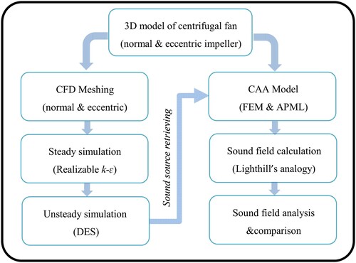
In this study, the noise prediction is based on the transient CFD results. The noise prediction procedure has two branches, as shown in Figure 1. Each branch is divided into two steps; namely, the simulation of the flow field by CFD and the CAA calculation of the sound field. The details of each step will be described in the following paragraphs.

Figure 1. Hybrid noise prediction procedure. 3D = three-dimensional; CFD = computational fluid dynamics; DES = detached eddy simulation; CAA = computational aeroacoustics; FEM = finite element method; APML = adaptive perfectly matched layer.

2.2. Internal flow field simulation model with eccentric impeller

2.2.1. Parameters of high-speed centrifugal fan

Figure 2 shows the structural components of the centrifugal fan. The centrifugal fan has an enclosed impeller with 24 blades, of which 12 are splitter blades. The detailed parameters are shown in Table 1. The rotating frequency (RF) and blade passing frequency (BPF) can be calculated by the following formulae: (1) $\begin{array}{rl}& f_{\text{RF}}={\displaystyle \frac{n}{60}}\end{array}$(1) (2) $\begin{array}{rl}& f_{\text{BPF}}={\displaystyle \frac{nZ}{60}}\end{array}$(2) where f_RF and f_BPF are RF and BPF, and n and Z are the rotating speed and number of main blades, respectively. Considering the rotating speed and blade number and style, the RF is about 113 Hz, with the first BPF at about 1357 Hz and the second BPF at about 2714 Hz.

Figure 2. Overview of the three-dimensional high-speed centrifugal fan model.

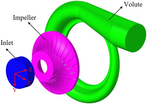
Table 1. Parameters of the centrifugal fan.

Rotating speed	6787 r/min
Rated flow rate	0.2873 kg/s
Inlet pipe length	25 mm
Inlet diameter	135 mm
Impeller diameter	268 mm
Blade number	12 + 12
Blade thickness	2.5 mm
Clearance between shroud and volute	1.5 mm

2.2.2. Governing equations and turbulence model

In current research, both the conventional Reynolds-averaged Navier–Stokes (RANS) equation and sophisticated methods such as DES and LES are usually adopted to calculate the internal flow field of the centrifugal fan (Lu et al., 2012; Maduka & Li, 2021; Meakhail & Park, 2005). Typically, the LES model can obtain a sufficiently accurate result for the noise prediction, although it requires substantially finer mesh than that needed for RANS (Sharma et al., 2020). When considering the whirling motion of the impeller’s inner flow field, however, it may bring some limitations to the use of LES owing to the high-resolution requirements for near-wall grids and the generation of structural hexahedral elements. Combining RANS and LES, the DES model is proposed (Spalart et al., 1997), based on the Spalart–Allmaras (S-A) model, and applied with good results over a range of Mach numbers. Delayed detached eddy simulation (DDES), resolving the gray area problem, is a relatively deep improvement of this initial DES (Spalart et al., 2006). It is likely to become the new standard version of DES (Spalart, 2009) and even the default selection in combination with certain RANS models in FLUENT.

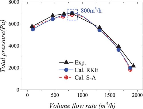
With its rapid development, the DES method has been extended for use in combination with other RANS models (Strelets, 2001), including the realizable k-ε model, which is the most successful modification of the widely used k-ε model (Ghalandari et al., 2019; Shih et al., 1995). The realizable k-ε provides more accurate predictions than the standard k-ε model, especially regarding the characteristics of rotational flows and boundary layers under strong adverse pressure gradients (Gao et al., 2018; Öztürk et al., 2019) . Based on the realizable k-ε model, the DES model has been well applied in many cases (Rajan & Cimbala, 2016; Guo et al., 2020; Zhang et al., 2008) and found to be numerically more stable than the widely applied S-A-based DES model in a simulation of an axial-channel rod (Basu et al., 2008). In this paper, we also compared the total pressure of the normal case obtained by S-A DDES and realizable k-ε DDES, as shown in Figure 3. From the comparison, the results calculated by realizable k-ε DDES shows a good correlation with the experimental results under most working conditions. Therefore, in this paper, the realizable k-ε DDES is expected to dominate the flow around the interacting blades and rotating impeller.

Figure 3. Comparison of the total pressure of the normal case obtained by Spalart–Allmaras (S-A) delayed detached eddy simulation (DDES) and realizable k-ε (RKE) DDES. Cal. = calculated; Exp. = experimental.

The modeled transport equations for k and ε in the realizable k-ε model are: (3) $\begin{array}{rl}\frac{\mathrm{\partial }}{\mathrm{\partial }t}(\rho k)+\frac{\mathrm{\partial }}{\mathrm{\partial }{x}_j}(\rho k{u}_j)& =\frac{\mathrm{\partial }}{\mathrm{\partial }{x}_j}\left[\left(\mu +\frac{{\mu }_t}{{\sigma }_k}\right)\frac{\mathrm{\partial }k}{\mathrm{\partial }{x}_j}\right]+G_k\\ & +G_b-\rho \epsilon -Y_M+S_k\end{array}$(3) and (4) $\begin{array}{rl}\frac{\mathrm{\partial }}{\mathrm{\partial }t}(\rho \epsilon )+\frac{\mathrm{\partial }}{\mathrm{\partial }{x}_j}(\rho \epsilon u_j)& =\frac{\mathrm{\partial }}{\mathrm{\partial }{x}_j}\left[\left(\mu +\frac{{\mu }_t}{{\sigma }_{\epsilon }}\right)\frac{\mathrm{\partial }\epsilon }{\mathrm{\partial }{x}_j}\right]\\ & +\rho C_{1}S\epsilon -\rho C_2\frac{{\epsilon }^2}{k+\sqrt{v\epsilon }}\\ & +C_{1\epsilon }\frac{\epsilon }{k}{C}_{3\epsilon }{G}_b+S_{\epsilon }\end{array}$(4) In the DES model, the realizable k-ε RANS dissipation term is modified such that: (5) $Y_k=\frac{\rho k^{\frac{3}{2}}}{l_{\text{des }}}$(5) where $l_{\text{des }}=min(l_{\text{rke }},l_{\text{les}})$, $l_{\text{rke}}=\frac{k^{\frac{3}{2}}}{\epsilon }$ and $l_{\text{les }}=C_{\text{des }}{\mathrm{\Delta }}_{\text{max }}$, in which ${\mathrm{\Delta }}_{\text{max}}$ is the grid spacing and $C_{\text{des }}$ is a calibration constant. To apply the DDES, the DES length scale $l_{\text{des}}$ is redefined as: (6) $l_{\text{des }}=l_{rke}-f_{d}max(0,l_{rke}-C_{des}{\mathrm{\Delta }}_{max})$(6)

2.2.3. Impeller eccentric motion model

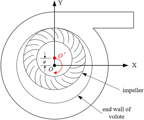
According to the centrifugal fan structure, the CFD calculation field is divided into three parts: the inlet pipe domain, the impeller domain and the volute domain. Interfaces are adopted to connect the rotating domain to the stationary domains. Figure 4 shows the diagram of the impeller motion model with eccentricity, where e is the eccentricity of the centrifugal fan impeller, representing the distance between the impeller’s geometric center O′ and rotating axis O, which maintains the same position relative to the volute. To investigate further how the eccentric effect of the impeller influences the flow pattern quantitatively, the non-dimensional parameter α is proposed, which is defined as follows: (7) $\alpha =\frac{e}{d}$(7) where d is the impeller diameter. In previous research, e is selected based on the actual data and the restriction of the maximum displacement of the rotor. For a centrifugal compressor, Broatch et al. (2015) measured the maximum value of e with about 67% of tip clearance and adopted this value in calculation. The study by Young et al. (2017) indicates that non-contact levels for e with 25–37.5% of tip clearance are common. In this paper, considering the restraint of clearance diameter in the normal case, three eccentric cases, named EC1, EC2 and EC3, have been studied, with α = 0.00062, 0.00125 and 0.00187, corresponding to e = 0.167, 0.33 and 0.5 mm.

Figure 4. Diagram of the impeller motion model considering the eccentric effect.

2.2.4. CFD mesh and boundary conditions

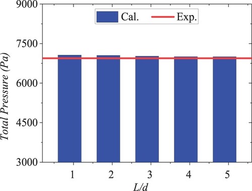
The code used for CFD computation is FLUENT 17.0, which is based on an unstructured grid, and the CFD mesh contains tetrahedral mesh in the core region and prism elements around the wall surface. The inlet and outlet pipes are extended to ensure full development of the flow, and different extension distances have been adopted in previous studies of centrifugal fans and compressors, varying from the pipe diameter to five times the diameter (Broatch et al., 2015; Chen et al., 2007; Liu et al., 2019). In this paper, the extension lengths of the inlet and outlet pipes are more than five times the diameter of pipeline, with the impact on the calculated results verified by a series of calculations (Figure 5). When the ratio of the extended length to the diameter of pipeline exceeds 4, the calculated total pressure tends to be stable, indicating that the previous length of pipe extension guarantees the full development of the flow.

Figure 5. Pressure rises with different extension lengths of the pipes. Cal. = calculated; Exp. = experimental.

The centrifugal fan in this paper has a shrouded impeller, and the shroud eliminates the tip clearance and associated tip leakage necessary with open or semi-open impellers. Thus, the tip clearance noise, which has been shown to have a weak effect on the noise characteristics in a centrifugal compressor (Navarro García, 2018; Zhong et al., 2021), would not exist in this study. Meanwhile, according to the tested noise spectrum described later, in Figures 20(a) and 25(a), there is also no disturbance by the upstream inlet gap, which would induce an additional tonal noise near the difference between the first BPF and the RF (Ottersten et al., 2021). Therefore, focusing on the eccentric effect, the clearance between the shield and impeller would have a weak influence in this paper and can be simplified in the calculations.

Figure 6 shows the CFD mesh for different domains. Based on the whirling model, the impeller is transported by the y-axis to some extent, to simulate the eccentric effect of the impeller and keep the shaft rotating concentrically. For an acceptable prediction of the boundary layer, 14 layers of the prism elements near the wall are generated, ensuring a larger thickness than that of the boundary layer. To ensure the effectiveness of the computation, the mesh independence analysis is carried out under rated working conditions, as shown in Figure 7. The difference between the simulation and test results in the last three cases can be omitted. Therefore, the mesh with 3.6 million elements is used to balance the capture of sound information and the calculation efficiency in the following investigations. Figure 8 shows the y-plus distribution of the whole calculation field with a maximum value of 4.18, which is acceptable.

Figure 6. Computational fluid dynamics (CFD) mesh in different domains: (a) impeller mesh; (b) wall mesh of impeller; (c) boundary layer of impeller; (d) cut plane of volute mesh.

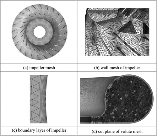
Figure 7. Mesh independence analysis. Exp. = experimental.

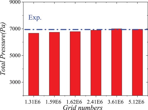
Figure 8. The y-plus distribution.

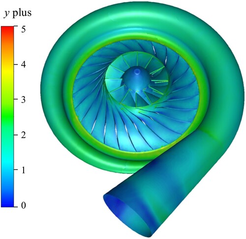
Table 2 summarizes the CFD settings applied in this study. The non-slip condition is applied to all the walls of the model. The rotation model in the steady calculation is a multiple reference frame (MRF). In transient calculations, the sliding mesh rotation model is adopted to keep the impeller domain rotating at a constant speed. The pressure inlet condition is applied at the inlet, with a value of 0 Pa. The outlet mass flow rate is set to 0.2873 kg/s to maintain the stability of the outlet flow. For the simulation of the fan, the characteristic Mach number described by the circumferential velocity of the blade tips is: (8) $Ma=\frac{u_2}{\text{c}}$(8) where u₂ is the circumferential speed of the blade tips and c is the speed of sound. According to the rotating speed and the diameter of the impeller, Ma = 0.548. Therefore, the flow is assumed to be compressible and the energy equation is solved with the continuity equation and the momentum equation. The steady calculation is carried out first to obtain a relatively reasonable flow field for the transient calculation. In unsteady calculation, the iteration in each time step is set to be 20. The definition of the time step and its number determine the resolution and the maximum frequency of the sound field calculation according to the sampling theorem. Considering the convergence of CFD and the noise frequency in which we are interested, the time step is set to 2.456e–5 s, which means that the impeller grid rotates by 1° per time step.

Table 2. Computational fluid dynamics settings.

Condition	Steady	Transient
Turbulence model	Realizable k-ε	Realizable k-ε DDES
Rotation model	MRF	Sliding mesh
Discretization schemes	Second order upwind	Second order upwind
Inlet condition	Pressure-inlet	Pressure-inlet
Outlet condition	Mass flow-outlet	Mass flow-outlet
Wall condition	No slip	No slip

Note: DDES = delayed detached eddy simulation; MRF = multiple reference frame.

2.3. Sound field simulation model

2.3.1. Lighthill’s acoustic analogy in variational formulation

In studies on fan noise prediction, both the BEM and FEM are usually adopted to consider the reflecting and scattering effects due to solid boundaries such as the volute and pipelines. When combining BEM, the sound analogy theory is used in the integral formulation of Lighthill’s analogy, represented by Curle’s analogy and the Ffowcs Williams–Hawkings (FW-H) equation. In this paper, the FEM is adopted and Lighthill’s acoustic analogy theory is used in a variational formulation, which was first derived by Oberai et al. (2000, 2012). Starting from the Lighthill equation, which is given as: (9) $\frac{{\mathrm{\partial }}^2}{\mathrm{\partial }{t}^2}(\rho -{\rho }_0)-a_0^2\frac{{\mathrm{\partial }}^2}{\mathrm{\partial }{x}_i\mathrm{\partial }{x}_i}(\rho -{\rho }_0)=\frac{{\mathrm{\partial }}^2{T}_{ij}}{\mathrm{\partial }{x}_i\mathrm{\partial }{x}_j}$(9) its strong variational statement can be obtained as: (10) $\begin{array}{rl}& {\int }_{\mathrm{\Omega }}\left(\frac{{\mathrm{\partial }}^2}{\mathrm{\partial }{t}^2}(\rho -{\rho }_0)-a_0^2\frac{{\mathrm{\partial }}^2}{\mathrm{\partial }{x}_i\mathrm{\partial }{x}_i}(\rho -{\rho }_0)-\frac{{\mathrm{\partial }}^2{T}_{ij}}{\mathrm{\partial }{x}_i\mathrm{\partial }{x}_j}\right)\delta \rho dx\\ & =0\mathrm{\forall }\delta \rho \end{array}$(10) where $T_{ij}$ is Lighthill’s tensor and $\delta \rho$ is a test function. Then, using integration by parts and substituting the total stress tensor: (11) $\sum {}_{ij}=\rho v_i{v}_j+(p-p_0){\delta }_{ij}-{\tau }_{ij}$(11) the variational formulation of Lighthill’s analogy is obtained: (12) $\begin{array}{rl}& {\int }_{\mathrm{\Omega }}\left(\frac{{\mathrm{\partial }}^2}{\mathrm{\partial }{x}^2}(\rho -{\rho }_0)\delta \rho +c_0^2\frac{\mathrm{\partial }}{\mathrm{\partial }{x}_i}(\rho -{\rho }_0)\frac{\mathrm{\partial }\delta \rho }{\mathrm{\partial }{x}_i}\right)dx\\ & =-{\int }_{\mathrm{\Omega }}\frac{\mathrm{\partial }{T}_{ij}}{\mathrm{\partial }{x}_j}\frac{\mathrm{\partial }\delta \rho }{\mathrm{\partial }{x}_i}dx+{\int }_{\mathrm{\Gamma }}\frac{\mathrm{\partial }{\mathrm{\Sigma }}_{ij}}{\mathrm{\partial }{x}_j}{n}_i\delta \rho dx\end{array}$(12) For the implementation, the unsteady CFD field is used to compute the right-hand side of Equation (12(12) $\begin{array}{rl}& {\int }_{\mathrm{\Omega }}\left(\frac{{\mathrm{\partial }}^2}{\mathrm{\partial }{x}^2}(\rho -{\rho }_0)\delta \rho +c_0^2\frac{\mathrm{\partial }}{\mathrm{\partial }{x}_i}(\rho -{\rho }_0)\frac{\mathrm{\partial }\delta \rho }{\mathrm{\partial }{x}_i}\right)dx\\ & =-{\int }_{\mathrm{\Omega }}\frac{\mathrm{\partial }{T}_{ij}}{\mathrm{\partial }{x}_j}\frac{\mathrm{\partial }\delta \rho }{\mathrm{\partial }{x}_i}dx+{\int }_{\mathrm{\Gamma }}\frac{\mathrm{\partial }{\mathrm{\Sigma }}_{ij}}{\mathrm{\partial }{x}_j}{n}_i\delta \rho dx\end{array}$(12) ), in which the first term represents the volume sound source, comprising convective fluxes, entropy variations and viscous stresses, and the second term represents the contribution of the surface sound source from an integral over the CFD boundaries. In the CAA model, those boundaries could be defined as the solid wall, including the rigid wall and vibrating wall, or the permeable surface which is located against the solid wall. For the centrifugal fan, the permeable face corresponds to the interface of the rotating and stationary domains, which is also defined as the control surface in the study by Caro et al. (2005). Thus, the surface source contribution needs to be evaluated only on the permeable surface to consider the sound source in the impeller, since it is equal to zero on all the other rigid boundaries (Caro et al., 2005). The CAA code used in this paper is ACTRAN 17.0.

Both the BEM and FEM methods are exact and contain no approximations. A significant difference between the two methods exists in their treatment of solid surfaces. As a purely explicit algorithm combining the free-field Green’s function, the BEM based on integral formulation uses the surface sound source to account for the effect of sound reflection by solid boundaries. Compared with the integral formulation, the variational formulation of Lighthill’s analogy is implicit and the effect of reflection by solid boundaries is accounted for by the acoustic solver. This has an inherent advantage in analyzing the acoustic characteristics of complicated structures as well as predicting sound transmission at low frequency. This simulation strategy was assessed in the study by Kierkegaard et al. (2016), in which the calculated results for a heating, ventilation and air-conditioning (HVAC) duct by this hybrid strategy were compared with the direct noise calculation results; the two strategies showed good correlation with the experimental result in both characteristic frequencies and broad band levels. Therefore, the variational formulation of Lighthill’s analogy would be very suitable for interior/ducted aeroacoustic problems, such as the centrifugal fan noise with an eccentric impeller studied in this paper.

2.3.2. Acoustic FEM model for centrifugal aerodynamic noise

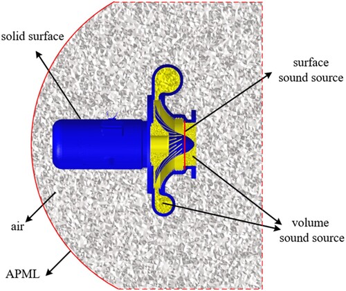
The acoustic FEM model for the centrifugal fan is shown in Figure 9. The sound source in the impeller is defined on the interface which connects the inlet region and the impeller. The other sound sources generated by flow in the inlet pipe and volute are defined in the volume sound source. The solid surface of the shell is set to be a reflecting surface. The adaptive perfectly matched layer (APML) is adopted to simulate the non-reflecting boundary, which avoids the interpolation order problem encountered in the infinite element method and the frequency range limitation by the element size in the use of perfectly matched layers. The analytical points of the sound spectrum are set up as several circular groups of field points with a distance of 1 m to the inlet.

Figure 9. Computational aeroacoustic (CAA) model for a high-speed centrifugal fan. APML = adaptive perfectly matched layer.

The sound information obtained by unsteady CFD results in the time domain can be transformed into the frequency domain using the convolution and fast Fourier transform (FFT). Then, the sound sources are interpolated into the acoustic mesh. The integrated interpolation method for sound source information mapping is utilized in the CAA model, which has a better accuracy than the traditional linear interpolation, especially when using the sparse CAA grid. The maximum frequency is about 2714 Hz, which is the BPF for 24 blades. The maximum calculation frequency is set to 3000 Hz, accompanied by the smallest wavelength of 0.113 m. In general, the CAA mesh should satisfy that there are six grids for each of the smallest wavelengths. The biggest grid for CAA is 0.015 m, which means that there are more than seven grids within the smallest wave. Thus, the fineness of the CAA mesh is acceptable.

3. Results and discussion

In this section, the validation of the performance is demonstrated by comparing the measured and simulated performance curves, including total pressure and efficiency. Then, the general distribution of the flow field and its frequency characteristics influenced by the eccentric impeller are analyzed. Following this, the measured and predicted sound field results are compared. Finally, the impact of the eccentric impeller on the acoustic characteristics of the fan will be discussed.

3.1. Validation of the CFD model

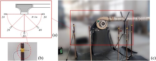
A test bench is set up to perform the experimental tests (Figure 10). The inlet is directly open to the atmosphere, and the outlet is connected to the outside with an outlet pipe. A flow adjustment unit is set at the end of the outlet to modify the flow rate of the fan. A pitot tube is installed on the outlet pipe to measure the static pressure and total pressure, and then the velocity of outlet flow can be calculated.

Figure 10. Test bench settings: (a) distribution of acoustic transducers; (b) B&K 4957 microphone; (c) experimental layout.

To consider the shaft whirling motion due to the eccentric effect, the experiment is conducted with and without dynamic balancing for the fan rotor. The coaxial degree of the bearings is checked by a 3D coordinate measuring machine to ensure a high axiality; thus, a perfect alignment can be ensured for the shaft. Running with an unbalanced impeller at high speed, the motion of the shaft is seen to contain the whirling motion. Therefore, the eccentric effect of the impeller can be realized to some extent.

The B&K test system is applied to measure the fan noise. Signals from noise transducers are transmitted to the data acquisition system B&K PULSE 13.6 and converted into digital signals. Finally, the data are analyzed in the PULSE front end on a laptop computer. The acoustic transducers used are B&K 4957 microphones, and the sound pressure measuring points are set at 1 m to the inlet of fan in a vertical plane, with a 45° interval between each transducer (Figure 10a and b). To fulfill the requirement of noise measurement, the centrifugal fan is set up on a steel bench at 1.3 m. The test environment contains no sound reflection except for the ground, which is covered by sound-absorbing material near the inlet. To prevent the acoustic characteristics of fan being contaminated by other sound sources, such as noise generated by the motor and pipe, the motor and the outlet pipe are isolated with acoustic cladding, which is composed of sound-absorbing material and stainless-steel casing (Figure 10c).

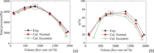
The key parameters of centrifugal fan performance are the total pressure (P_t) and internal efficiency (η) (Chen et al., 1996; Qi et al., 2009): (13) $\eta =\frac{Q{P}_t}{2\pi nT}$(13) where n, T, Q and P_t are the rotating speed, torque, volumetric flow rate and total pressure, respectively. In this paper, the performance curves of total pressure and efficiency are also compared with the experimental results for the validation of the CFD model, as shown in Figure 11. The calculated result of the normal impeller case correlates well with the experimental results, especially at the rated condition (marked by a dashed box), indicating that the CFD result is reliable. For the eccentric case, which is EC3, both the calculated total pressure and efficiency decrease in the whole range of the calculated flow rate, and the performance becomes worse with the increase in the deviation from the rated condition. Based on these comparisons, the normal-impeller centrifugal fan has a better performance than the eccentric one, which is in line with the existing research on centrifugal compressors.

Figure 11. Comparison of calculated (Cal.) and experimental (Exp.) performance curves: (a) total pressure; (b) internal efficiency.

3.2. Flow field analysis

The calculated results of both normal and eccentric impeller cases are analyzed in this section, including steady analysis and unsteady analysis. The velocity, pressure and turbulence kinetic energy (TKE) distribution are compared for different cases. The key positions of turbulent fluctuation in the flow field are located, thus enabling the sound source type and its intensity to be estimated.

3.2.1. Steady analysis

For more accurate analysis of the flow pattern and the field distribution, the transient calculation result at the last time step (i.e. the 0 T time step), rather than the steady calculation result, is adopted for the qualitative analysis. The calculated result of EC3 is used for the comparison with the normal case, aiming to clearly reflect the impeller-eccentric effect. Defining the blade height direction as from hub to shroud, the vortices at the span plane of 50% blade height under different condition are compared (Figure 12). Owing to the whirling motion of the eccentric impeller, the direction of the impeller outflow changes with the rotation, leading to a varying angle between the outflow direction and the volute tongue. As a result, distinct low-speed areas occur at the left side of the volute and near the volute tongue, as shown in regions a and b in Figure 12.

Figure 12. Velocity vector comparison.

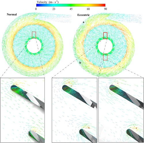
The near-shroud partial field of the velocity vector at the leading edge (LE) of the blades is shown to reflect the eccentric effect. According to the calculation time step, the upper region has the smallest gap between the impeller and the volute tongue. Compared to the same position in the normal impeller, the attack angle of incoming flow is changed, resulting in a stronger flow separation on the suction surface (SS). The velocity near the shroud on the LE in EC3 is larger, while the mean velocity of the incoming flow for the splitter blades is smaller. In the lower region, the flow separation on the SS is alleviated but the low-speed region still exists. In other words, the eccentric effect induces a variation in the attack angle and therefore a change in the flow separation position, increasing the uneven distribution of velocity in both the impeller and the volute.

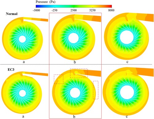
The pressure contours of the whole region at 10%, 50% and 90% blade height are shown in Figure 13, labeled a, b and c. In each case, the pressure contours with different blade heights have a similar distribution law. Comparing the 50% blade height result, the pressure with an eccentric impeller shows a relatively non-uniform distribution, especially a large pressure gradient near the volute tongue as well as a high-pressure region at the right side of the volute (marked by dashed lines). In addition, the non-uniformity of the pressure distribution in the volute is similar to the distribution of the low-speed area in Figure 12.

Figure 13. Pressure contour on the span plane at (a) 10%, (b) 50%, and (c) 90% blade height.

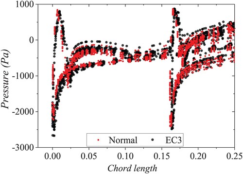
In the impeller, the eccentric effect also influences the blade loading distribution. Figure 14 shows the blade loading at the span plane of 50% blade height. The blade loading along the 0–0.2 chord length, which is from LE to TE, reflects the pressure distribution of the LE region of both the main blades and the splitter blades. Compared with that of the normal impeller, the blade loading in the eccentric impeller has a larger range, which could be induced by a stronger flow instability near the LE area.

Figure 14. Blade loading comparison for 0–0.2 chord length (50% blade height).

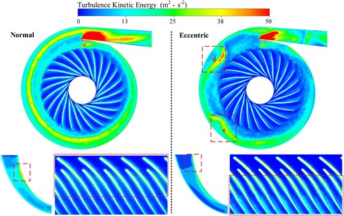
As a significant parameter related to both dipole and quadrupole noise, the TKE can reflect the influence of the eccentric impeller on the noise generation. Figure 15 shows the comparison of TKE in both the volute and impeller domains at the span plane of 50% blade height. In the volute domain, the TKE becomes non-uniformly distributed in the eccentric case and shows new concentrations in areas a and b. In the impeller domain, the TKE mainly distributes near the SS of the blades within 0–0.6 chord length in the normal case. In the eccentric impeller, this changes to the 0.4–1 chord length and extends from the SS to the pressure surface (PS) in some regions. This is reasonable when considering the low-speed incoming flow for the splitter blades shown in Figure 12. Moreover, from the meridional view, the high TKE region on the shroud line changes from the LE of the splitter blade to the LE of the main blade, which is also coincident with the varying attack angle for the main blades shown in the near-shroud partial field in Figure 12. In other words, the trend in the variation of the TKE distribution reflects the unsteadiness of the velocity influenced by the impeller eccentricity; thus, it may lead to a rise in turbulence noise in both the impeller domain and the volute domain.

Figure 15. Turbulence kinetic energy distribution comparison (50% blade height span plane).

3.2.2. Unsteady analysis

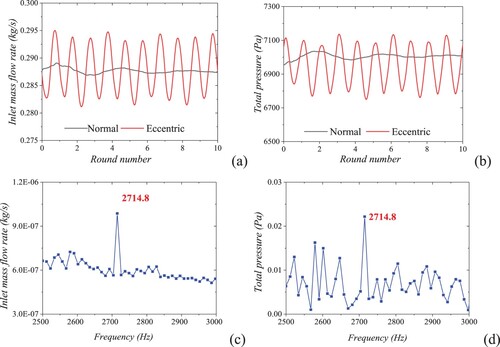
The unsteady analysis focuses on the pressure fluctuation and sound source generation at different locations induced by the impeller-eccentric effect. The calculated result of EC3 is used to represent the eccentric case. First, the inlet mass flow rate and outlet total pressure with normal and eccentric impellers at rated conditions are analyzed. Considering the eccentric effect, the whirling motion of the impeller will lead to regular changes in the distance between the impeller center and the volute tongue, from low to high and to low. Therefore, the inlet mass and outlet pressure fluctuate at the RF (Figure 16a and b). Owing to the effect of the volute, which influences the velocity field of the impeller outlet, as well as the prolonged pipeline to ensure the full development of flow, the high frequency fluctuations of both the inlet mass flow rate and outlet pressure fluctuation are decreased dramatically, such as in the result of the normal case at the second BPF (Figure 16c and d).

Figure 16. Inlet mass and outlet pressure in 10 rounds: (a) inlet mass comparison; (b) outlet total pressure; (c) inlet mass fluctuation at the second blade passing frequency (BPF) in the normal case; (d) outlet pressure fluctuation at the second BPF in the normal case.

To investigate the pressure fluctuation, which indicates the sound source to a certain extent, monitoring points are set in the impeller and volute domains to obtain the pressure information at crucial positions. Monitoring points B1–B8 are located around the outlet of the impeller with a 45° interval of angle, and points R1, R2 and R3 are at different heights in one channel and rotate with the impeller, as shown in Figure 17. By FFT, the monitoring results are transformed into the frequency domain. The comparison of pressure fluctuations in both the normal and eccentric cases is given in Figure 18. In the impeller, as shown in Figure 18(a), the pressure fluctuation only contains the RF and its harmonics, with the largest pressure amplitude occurring at the RF in each spectrum. Comparing each point, the eccentric impeller induced a stronger pressure fluctuation than the normal impeller, which may lead to increased sound source generation at the RF.

Figure 17. Setting of monitoring points.

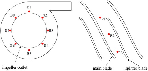
Figure 18. Pressure fluctuation at measuring points (MPs) in the frequency domain: (a) impeller passage; (b) normal impeller outlet; (c) eccentric impeller outlet; (d) impeller outlet with different eccentricities.

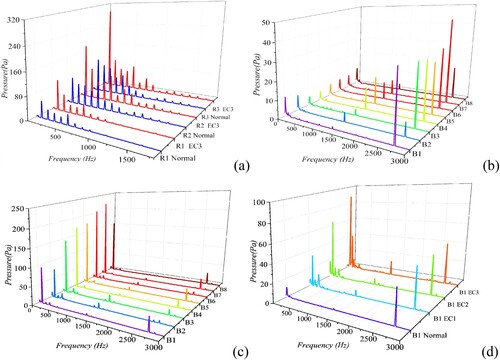
Meanwhile, in the volute domain, the pressure fluctuation shows enormous differences between the normal and eccentric cases, as shown in Figure 18(b). In the eccentric case, the amplitude at the RF becomes to dominant frequency and rises to at least 10 times larger than in the normal condition, while the amplitude at the first BPF and second BPF maintains the same order of magnitude. Taking B1 as an example, the pressure fluctuation at RF rises with the increase in eccentricity (Figure 18c), while the amplitudes at the first BPF and second BPF show only a little change. This is reasonable when considering the stronger rotor–stator interaction at the TE of the whirling impeller and the stronger pressure fluctuation transmitted from the impeller passage, which would increase logically with the increase in eccentricity.

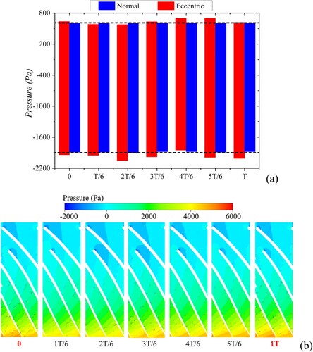
To investigate further the impeller-eccentric effect on the rotor–stator interaction, Figure 19(a) shows the blade loading in the 0–0.2 chord length, representing the region near the LE which makes a large contribution to the noise spectrum. Comparing the results at different times in the last round, the pressure range of the normal case, marked with a dotted line, is smaller than that of the eccentric case at each time point, and its fluctuation can also be ignored. Figure 19(b) shows the variation trend with the eccentric impeller in the last round. The negative pressure region around the LE first increases and then reduces with the increase in time. And the pressure contour at 1 T has almost the same distribution as that at 0 T, showing an obvious periodic variation trend.

Figure 19. Variation of blade loading in one spin of the impeller (0–0.2 chord length): (a) blade loading range comparison for 0–0.2 chord length; (b) pressure contour at the leading edge of the eccentric impeller in one spin.

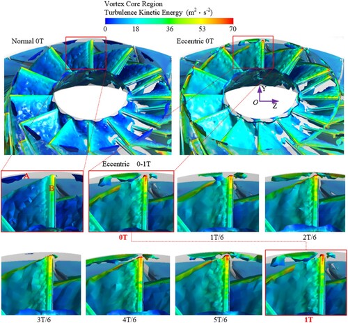
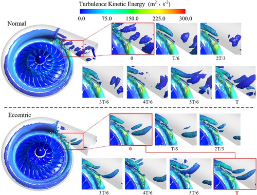
Meanwhile, the vortex structure in the impeller is shown in Figure 20, including the normal case at 0 T and the eccentric case with different instants in the last round. The Q criterion is adopted, with Q_Crit= 0.01, and the figure is colored with TKE. The partial field at the LE, which has the smallest gap to the volute tongue, is enlarged in both conditions. In the normal condition, the vortex distribution near the shroud is labeled ‘A’ in the enlarged partial field. In the eccentric impeller at 0 T, the vortex generation in area A tends to be unevenly distributed along the circumferential direction compared to the normal condition. Another significant difference is that the TKE on the LE near the shroud in the eccentric impeller has a higher value than in the normal impeller, which is labeled ‘B’ in the enlarged field. Moreover, aiming at the partial field, the vortex distribution in area A and TKE in area B vary with the change in time, i.e. the change in angle. Both of them first decrease and then increase, and the distribution at 1 T shows little difference from 0 T. In other words, the eccentricity of the impeller increases the unsteadiness of the turbulence near the LE and results in an obvious periodicity in the variation of TKE and the vortex structure, which leads to a stronger rotor–stator interaction and increased sound source generation at the LE.

Figure 20. Vortex generation in the impeller with different instants.

The turbulence and vortex generation in the volute are shown in Figure 21. The Q criterion is also adopted, with Q_Crit= 0.01, and the figure is colored with TKE. In the volute domain, the high TKE region appears near the volute tongue, and the partial field at the key position is enlarged at different times in the last round. From 0 T to 1 T, the vortex structures detach from the volute tongue in both cases. However, in the case of the eccentric impeller, the vortex structure near the volute tongue at 0 T and 1 T shows the same distribution law, indicating a much more remarkable periodicity at the RF than that in the normal condition. Thus, the eccentric impeller induces a regular vortex shedding near the volute tongue at the RF, which generates more turbulent noise at the RF and its harmonics.

Figure 21. Vortex structure comparison in one round.

3.3. Sound field analysis

3.3.1. Sound field analysis with normal impeller

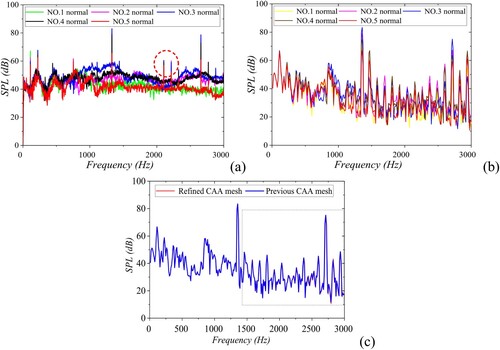
In the case of the normal impeller, the numerical and experimental results of the sound pressure level (SPL) at measuring points (MPs) 1–5 are given in Figure 22. Basically, the noise spectrum of the centrifugal fan includes a group of the discrete noise and certain broadband noise (Holste & Neise, 1993; Mao et al., 2021). Figure 22(a) and (b) shows, respectively, the experimental and calculated results of the noise spectrum. The frequency spectrum consists of peaks at the RF, second RF, BPF, which is 12 times RF, and second BPF. The SPL reaches the highest level at the BPF, which becomes the dominant peak. The peaks at certain frequencies, marked in Figure 22(a), are generated by motor electromagnetic excitation, which could not be fully eliminated in the measurement. Based on the hybrid CAA method, the prediction accuracy is ensured by the CAA model and the sound source accuracy. A calculation with a finer CAA mesh, which has twice the number of the previous grids, is conducted (Figure 22c), indicating few improvements in accuracy when using the finer mesh. Thus, the previous CAA mesh can guarantee the demand for accuracy.

Figure 22. Frequency domain results at computational fluid dynamics (CFD) monitoring points: (a) experimental result at measuring points (MPs) 1–5; (b) calculated result at MPs 1–5; (c) noise spectrum comparison with finer computational aeroacoustic (CAA) mesh at monitoring point NO.3. SPL = sound pressure level.

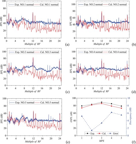
To validate the accuracy of the whole simulation strategy, the experimental and numerical results of the normal case at each measuring point are compared in Figure 23(a)–(e). For the convenience of identifying the characteristic frequency, the horizontal axis is labeled in multiples of the RF. The frequency resolutions of the experimental and calculated results are 1 and 11.3 Hz, respectively. From the comparison, the calculated spectrum shows a relatively good correlation with the measured noise spectrum at some crucial characteristic frequencies as well as the broadband noise in the low-frequency range. The comparison of the overall sound pressure level (OSPL) at MPs 1–5 is shown in Figure 23(f), with the discrepancy among MPs 1–5 being no larger than 6.1 dB and a minimum value of 1.4 dB. Considering the dominant effect by characteristic frequencies in the noise spectrum, the comparison of calculated and experimental results at each measuring point further validates both the CFD and CAA simulation models in this study.

Figure 23. Comparison between calculated (Cal.) and experimental (Exp.) results of a normal impeller at measuring points (MPs) 1–5: (a) NO.1; (b) NO.2; (c) NO.3; (d) NO.4; (e) NO.5; (f) overall sound pressure level (OSPL) comparison at MPs 1–5. RF = rotating frequency; SPL = sound pressure level.

However, the discrepancy of broadband noise implies that the capability of obtaining a sufficiently accurate solution of aerodynamic noise for the present simulation strategy is still limited, especially in the high-frequency range. The possible reasons for the discrepancy are as follows. First, the length scale of the mesh for DES to discretize the flow field is still coarser than that required in more sophisticated methods, such as LES and direct numerical simulation (DNS). It does not have the ability to accurately simulate the high-frequency pressure fluctuation induced by the eddy with small length scales. Second, in this manuscript, the model neglects the noise generated by the vibration noise source. This simplification is reasonable in the low-frequency range. However, the acoustic energy generated and scattered by structural vibration may make an important contribution at high frequencies and could not be fully eliminated in the measurement. Third, the propagating noise is affected by the synergy of flow and sound fields. In the present investigation, the hybrid CAA strategy does not take this coupling effect into consideration and is also likely to increase the discrepancy between the calculated and measured noise spectra.

It is still a challenge to accurately resolve the aerodynamic sound source, especially of eddies with small size and high frequency. The analytical model for the generation, distribution and propagation of aerodynamic noise should be advanced in future research.

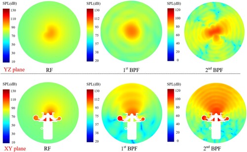
By attracting the cut plane of the sound pressure distribution, the sound radiation directivity is analyzed at crucial frequencies, as shown in Figure 24. The sound field distribution on the vertical plane of the inlet varies with the increase in frequency, with a similar phenomenon also existing in the study by Liu et al. (2019). At low frequencies, the sound wavelength is larger than the length of the inlet diameter (135 mm), and the transmitting form of sound waves at the RF would be spherical waves. With the rise in frequency, the sound wave diffraction effect weakens with the decrease in sound wavelength, and the sound field direction will gradually concentrate towards a range of angles. Therefore, significant reflecting and scattering effects by the volute structure appear at 2715 Hz, which is clearer than that at the RF and first BPF.

Figure 24. Sound directivity in the normal case. RF = rotating frequency; BPF = blade passing frequency; SPL = sound pressure level.

3.3.2. Sound field analysis with eccentric impeller

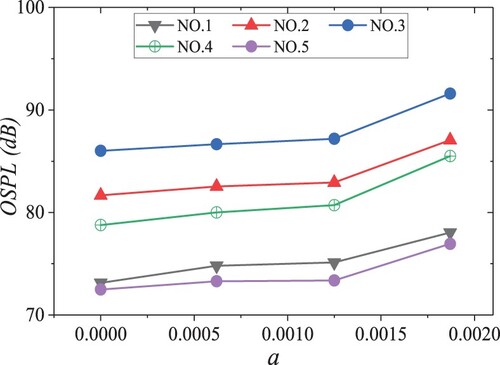
The sound field results with the eccentric impeller are calculated based on the transient CFD results of each eccentric condition. Figure 25 shows the influence of the non-dimensional parameter α on the OSPL results, including the normal case, EC1, EC2 and EC3. With the increase in α, the OSPL at each measuring point rises, with a similar trend between them, keeping the order as NO.3, NO.2, NO.4, NO.1 and NO.5. The variation trend fits well with the more drastic changes in vortex structure and TKE distribution shown in the unsteady analysis of the eccentric case in Figures 20 and 21, which indicate increased sound source generation. Meanwhile, the rising trend of OSPL is also similar to that of the pressure fluctuation amplitude in both the impeller and volute shown in Figure 18, which is reasonable since the pressure fluctuation also corresponds to the noise generation, to some extent.

Figure 25. Overall sound pressure level (OSPL) results at measuring points (MPs) 1–5 under different impeller eccentricities.

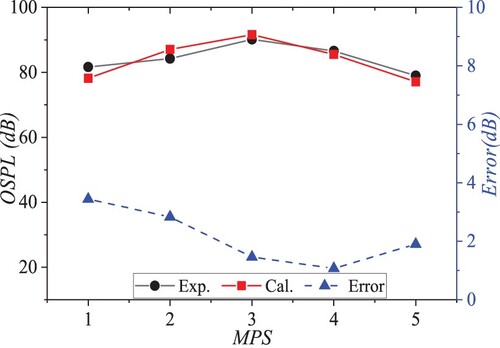
To maintain consistency with the unsteady flow field analysis, the CAA result of EC3 is used for analysis. Figure 26 shows the experimental and numerical results at MPs 1–5 with the eccentric impeller. Similarly to the normal case, both experimental and simulated noise spectra of the eccentric case consist of the dominant peaks at the RF, BPF and second BPF. However, the SPL at the RF shows significant changes. In the experiment of the eccentric case (Figure 26a), the maximum, magnitude at the RF is 73.9 dB, which is 6.8 dB larger than the maximum value of 67.1 dB in the normal case (Figure 22a). For the calculated result (Figure 26b), the maximum magnitude at the RF also shows a 4.2 dB rise from the normal case, which has a maximum value of 66.8 dB (Figure 22b). Thus, the significant increase in the SPL at the RF in both the calculated and experimental results is consistent with the periodic change in flow field at the RF analyzed in Section 3.2.2. Meanwhile, according to the previous investigation and the sound directivity analyzed in Figure 24, the sound wave reflecting and scattering effect would strengthen along with the increase in frequency, resulting in a different sound field distribution. Therefore, in Figure 26(a), the experimental results at each monitoring point show some discrepancy with regard to both the amplitude and the trend, which is also reflected in the calculated result in Figure 26(b). The overall SPL with the eccentric impeller at MPs 1–5 obtained by experiment and calculation is shown in Figure 27. The largest error of total SPL among MPs 1–5 is 3.6 dB, while the minimum error is 1.1 dB, indicating a good accuracy of the simulation strategy in general.

Figure 26. Frequency spectrum with an eccentric impeller at measuring points (MPs) 1–5: (a) experimental results; (b) calculated results. SPL = sound pressure level.

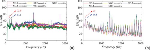
Figure 27. Total overall sound pressure level (OSPL) with an eccentric impeller at measuring points (MPs) 1–5.

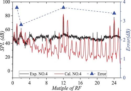
The impeller-eccentric effect on the noise spectrum is analyzed by an elaboration of the result at measuring point NO.4, which can reflect the scattering effect at high frequency more accurately than NO.1 and NO.5. It is also less influenced by the reflecting effect of the outlet pipeline, which cannot be fully simulated in the calculations. In the experimental result, the spectrum of the eccentric case shows similar characteristics to the normal case, whereas the SPL at the crucial peaks rises obviously, especially at the RF, second BPF and frequencies lower than the RF, which are marked with blue rectangles in Figure 28(a). Figure 28(b) shows the calculated result comparing the normal and eccentric cases. As shown in the blue rectangles, the calculated result shows a similar variation trend to the change in experimental results, successfully capturing the impact of the eccentric impeller on the increase in SPL at crucial frequencies. the increase in magnitude at the first BPF is acceptable compared with the experimental result, as shown in Figure 29. The maximum error at crucial frequencies is no larger than 3.7 dB, which further illustrates the high accuracy of the numerical simulation in the whole frequency range.

Figure 28. Eccentric effect on NO.4 noise spectrum: (a) experimental (Exp.) results; (b) calculated (Cal.) results. RF = rotating frequency; SPL = sound pressure level.

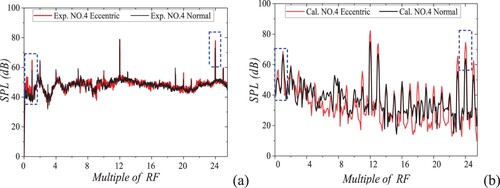
Figure 29. Experimental (Exp.) and calculated (Cal.) results at NO.4 (eccentric impeller). RF = rotating frequency; SPL = sound pressure level.

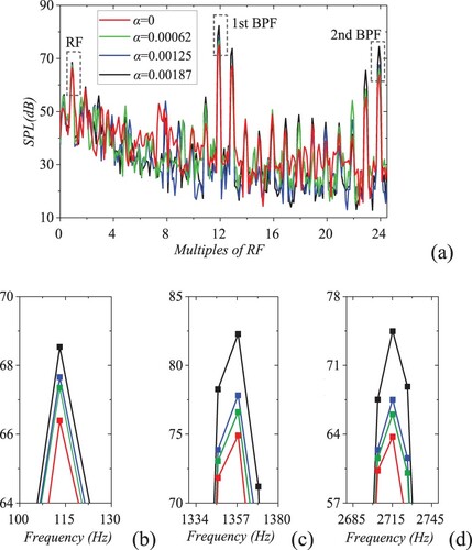
To study further the impeller-eccentric effect on the noise spectrum, the varying trend in the noise spectrum at measuring point NO.4 under different values of α is analyzed in Figure 30. In general, the calculated noise spectrum increases with the increase in eccentricity, and the most significant change is the magnitude at characteristic frequencies, including the RF, first BPF and second BPF. The change at characteristic frequencies correlates well with the trend in OSPL in Figure 25.

Figure 30. Noise spectrum at NO.4 measuring point with different impeller eccentricities: (a) noise spectrum at the whole frequency range; (b) partial result at rotating frequency (RF); (c) partial result at first blade passing frequency (BPF); (d) partial result at second BPF. SPL = sound pressure level.

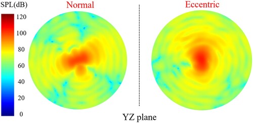
The impeller-eccentric effect on sound directivity is also analyzed, with the most significant change appearing at the sound field at the second BPF (Figure 31). On the YZ cut plane, the eccentric effect changed the sound radiation directivity into roughly three directions, which would usually be four directions in the normal case. Thus, the impeller-eccentric effect can influence the uniform distribution of the sound field, which may lead to more irregular changes for the noise spectrum at different measuring points.

Figure 31. Eccentric effect on sound directivity at the second blade passing frequency (BPF). SPL = sound pressure level.

3.3.3. Sound source characteristics and contribution

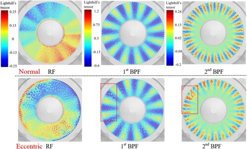
Representing the acoustic intensity, the magnitude of the divergence of Lighthill’s tensor at crucial frequencies is given in Figure 32. Indicated by the red dashed line, the magnitude of Lighthill’s tensor in the eccentric case (EC3) shows a circumferential non-uniform distribution compared with the normal case. From the transient computation results analysis, the whirling motion of the impeller results in the unsteadiness of the cut of turbulence by the LE, which leads to stronger flow separation and increased generation of the vortex structure in the impeller flow path and volute (Figures 20 and 21). Meanwhile, a stronger rotor–stator interaction is accompanied by the whirling motion of the impeller, which induces a stronger flow of unsteadiness in the volute region. Thus, the varying trend of sound source intensity and the stronger unsteadiness flow validate each other. The introduction of the impeller’s whirling motion is the predominant source mechanism for the increase in SPL in the noise spectrum.

Figure 32. Lighthill’s surface contribution with an eccentric impeller. RF = rotating frequency; BPF = blade passing frequency.

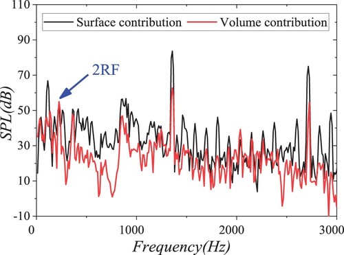
The sound spectrum of the centrifugal fan obtained by simulation consists of the contribution by Lighthill’s surface and volume, i.e. the noise contributed by the impeller and other parts. Figure 33 shows the contributions to the noise spectrum by different parts. The contribution of the surface sound source is much more than that of the volume sound source at almost all frequencies, whereas the second RF is mainly contributed to by the volume source. Moreover, the volume and surface contributions are almost the same at frequencies lower than the RF. This illustrates that the use of a volume source can help to refine the prediction of the noise spectrum of the centrifugal fan.

Figure 33. Sound source contribution with a normal impeller at NO.3 measuring point. RF = rotating frequency; SPL = sound pressure level.

4. Conclusion

A hybrid strategy combining DES and Lighthill’s analogy implemented by the acoustic FEM is presented to investigate the flow field characteristics and aerodynamic noise of centrifugal fans focusing on the impeller-eccentric effect, which has rarely been explored numerically before. The key sound source region sensitive to the impeller-eccentric effect is located, and the sound source, except for the impeller, is found to make a significant contribution at the second RF and frequencies lower than the RF. This study provides a foundation for identifying changes in the noise spectrum induced by impeller-eccentric effects resulting from installation and machining errors. The main conclusions are as follows:

1. When considering the eccentric effect of the impeller, the aerodynamic noise spectrum shows an obvious increase at the RF as well as its lower frequencies and at the second BPF, which can be observed in both calculations and experiments.

2. The impeller-eccentric effect changes the attack angle of incoming flow periodically, which leads to a stronger flow separation at the LE of the main blades and a lower mean velocity of incoming flow for the splitter blades. Accordingly, the pressure, TKE and vortex generation in both the impeller and the volute show an uneven distribution and periodic changes in the RF, and the performance of the centrifugal fan declines.

3. The magnitude of Lighthill’s tensor in an eccentric impeller has a circumferential non-uniform distribution in a similar position to the high TKE region in the flow field. The changes of the sound source intensity and flow field characteristics can validate each other.

4. The OSPL rises gradually with the increase in eccentricity. It also results in significant changes in sound directivity at characteristic frequencies, which vary from four directions to three at the second BPF.

5. Improvements and future direction

However, there are still limitations in this paper. For many practical restrictions, it would be more convincing if the sound field could be measured in an anechoic chamber. If possible, visualization measurement of the flow field inside the fan under laboratory conditions will be important in the next phase of work.

Disclosure statement

No potential conflict of interest was reported by the authors.

Additional information

Funding

This work was supported by the National Natural Science Foundation of China [grant number 51806042].

References

- Abadi, A. M. E., Sadi, M., Farzaneh-Gord, M., Ahmadi, M. H., & Chau, K. W. (2020). A numerical and experimental study on the energy efficiency of a regenerative heat and mass exchanger utilizing the counter-flow Maisotsenko cycle. Engineering Applications of Computational Fluid Mechanics, 14(1), 1–12. https://doi.org/10.1080/19942060.2019.1617193
- Alford, J. S. (1965). Protecting turbomachinery from self-excited rotor whirl. Journal of Engineering for Power, 87(10), 333–343. https://doi.org/10.1115/1.3678270
- Azzam, T., Paridaens, R., Ravelet, F., Khelladi, S., Oualli, H., & Bakir, F. (2017). Experimental investigation of an actively controlled automotive cooling fan using steady air injection in the leakage gap. Proceedings of the Institution of Mechanical Engineers, Part A: Journal of Power and Energy, 231(1), 59–67. https://doi.org/10.1177/0957650916688120
- Ballesteros-Tajadura, R., Hurtado-Cruz, J. P., & Santolaria-Morros, C. (2006). Numerical calculation of pressure fluctuations in the volute of a centrifugal fan. Journal of Fluids Engineering, 128(2), 359–369. https://doi.org/10.1115/1.2170121
- Basu, D., Das, K., Painter, S. L., Howard, L. D., & Green, S. T. (2008). Assessment of DES multiscale turbulence models for prediction of flow and heat transfer in an axial-channel rod configuration. International conference on nuclear engineering, Orlando, FL, USA, May 11–15, 2008.
- Broatch, A., Galindo, J., Navarro, R., García-Tíscar, J., Daglish, A., & Sharma, R. K. (2015). Simulations and measurements of automotive turbocharger compressor whoosh noise. Engineering Applications of Computational Fluid Mechanics, 9(1), 12–20. https://doi.org/10.1080/19942060.2015.1004788
- Burgmann, S., Fischer, T., Rudersdorf, M., Roos, A., Heinzel, A., & Seume, J. (2017). Development of a centrifugal fan with increased part-load efficiency for fuel cell applications. Renewable Energy, 116, 815–826. https://doi.org/10.1016/j.renene.2017.09.075
- Cao, W. D., Yao, L. J., Liu, B., & Zhang, Y. N. (2017). The influence of impeller eccentricity on centrifugal pump. Advances in Mechanical Engineering, 9(9), 1–17. https://doi.org/10.1177/1687814017722496
- Caro, S., Ploumhans, P., Gallez, X., Sandboge, R., & Matthes, M. (2005). A new CAA formulation based on Lighthill’s analogy applied to an idealized automotive HVAC blower using AcuSolve and ACTRAN/LA.
- Chen, J., He, Y., Gui, L., Wang, C., Chen, L., & Li, Y. (2018). Aerodynamic noise prediction of a centrifugal fan considering the volute effect using IBEM. Applied Acoustics, 132(March), 182–190. https://doi.org/10.1016/j.apacoust.2017.10.015
- Chen, P., Nayagam, M. S., & Bolton, A. N. (1996). Unstable flow in centrifugal fans. Journal of Fluids Engineering, 118(1), 128–133. https://doi.org/10.1115/1.2817490
- Chen, S. Y., Xi, S., & Wang, C. X. (2007). Three-dimensional numerical simulation of the internal flow in the centrifugal fan. Fluid Machinery, 9(9), 22–25. https://doi.org/10.3969/j.issn.1005-0329.2007.09.006
- Edward, C., Andrea, C., Francesco, J., Fabio, M. Z., & avide, P. D. (2018). Effect of rotor deformation and blade loading on the leakage noise in low-speed axial fans. Journal of Sound and Vibration, 433, 99–123. https://doi.org/10.1016/j.jsv.2018.07.005
- Gao, X. P., Zhang, H., Liu, J. J., Sun, B. W., & Tian, Y. (2018). Numerical investigation of flow in a vertical pipe inlet/outlet with a horizontal anti-vortex plate: Effect of diversion orifices height and divergence angle. Engineering Applications of Computational Fluid Mechanics, 12(1), 182–194. https://doi.org/10.1080/19942060.2017.1387608
- Ghalandari, M., Ziamolki, A., Mosavi, A., Shamshirband, S., Chau, K. W., & Bornassi, S. (2019). Aeromechanical optimization of first row compressor test stand blades using a hybrid machine learning model of genetic algorithm, artificial neural networks and design of experiments. Engineering Applications of Computational Fluid Mechanics, 13(1), 892–904. https://doi.org/10.1080/19942060.2019.1649196
- Guo, Z. J., Liu, T. H., Hemida, H., Chen, Z. W., & Liu, H. K. (2020). Numerical simulation of the aerodynamic characteristics of double unit train. Engineering Applications of Computational Fluid Mechanics, 14(1), 910–922. https://doi.org/10.1080/19942060.2020.1784798
- Holste, F., & Neise, W. (1993). Spring Workshop Center of Acoustics and Vibration. Pennsylvania State University, Pennsylvania, PA, USA, 22–23 April, DLR.
- Huang, J. Y., Zhang, K., Li, H. Y., Wang, A. R., & Yang, M. Y. (2021). Numerical simulation of aerodynamic noise and noise reduction of range hood. Applied Acoustics, 175(3), 107806. https://doi.org/10.1016/j.apacoust.2020.107806
- Kameier, F., & Neise, W. (1997). Rotating blade flow instability as a source of noise in axial turbomachines. Journal of Sound and Vibration, 203(5), 833–853. https://doi.org/10.1006/jsvi.1997.0902
- Kang, Y. S., & Kang, S. H. (2010). Prediction of the nonuniform tip clearance effect on the axial compressor flow field. Journal of Fluids Engineering, 132(5), 9. https://doi.org/10.1115/1.4001553
- Kierkegaard, A., West, A., & Caro, S. (2016, 30 May–1 June). HVAC noise simulations using direct and hybrid methods. 22nd AIAA/CEAS Aeroacoustics conference, Lyon, France.
- Kim, H. S., Cho, M. H., & Song, S. J. (2003). Stability analysis of a turbine rotor system with Alford forces. Journal of Sound and Vibration, 260(4), 167–182. https://doi.org/10.1016/S0022-460X(02)00926-4
- Kissner, C. A., & Guérin, S. (2019). Influence of wake and background turbulence on predicted fan broadband noise. AIAA Journal, 58(8), 1–14. https://doi.org/10.2514/1.J058148
- Krain, H. (2005). Review of centrifugal compressor’s application and development. Journal of Turbomachinery, 127(1), 25–34. https://doi.org/10.1115/1.1791280
- Li, W., Ji, L., Shi, W., Zhou, L., Agarwal, R., & Mahmouda, E. (2020). Numerical investigation of internal flow characteristics in a mixed-flow pump with eccentric impeller. Journal of the Brazilian Society of Mechanical Sciences and Engineering, 42(9), 1–19. https://doi.org/10.1007/s40430-020-02536-7
- Liu, C., Cao, Y., Zhang, W., Ming, P., & Liu, Y. (2019). Numerical and experimental investigations of centrifugal compressor BPF noise. Applied Acoustics, 150(July), 290–301. https://doi.org/10.1016/j.apacoust.2019.02.017
- Liu, H., Jiang, B. Y., Wang, J., Yang, X. P., & Xiao, Q. H. (2021). Numerical and experimental investigations on non-axisymmetric D-type inlet nozzle for a squirrel-cage fan. Engineering Applications of Computational Fluid Mechanics, 15(1), 363–376. https://doi.org/10.1080/19942060.2021.1883115
- Liu, Q. H., Qi, D., & Mao, Y. J. (2006). Numerical calculation of centrifugal fan noise. Proceedings of the Institution of Mechanical Engineers, Part C: Journal of Mechanical Engineering Science, 220(8), 1167–1177. https://doi.org/10.1243/09544062JMES211
- Lu, F. A., Qi, D. T., Wang, X. J., Zhou, Z., & Zhou, H. H. (2012). A numerical optimization on the vibroacoustics of a centrifugal fan volute. Journal of Sound and Vibration, 331(10), 2365–2385. https://doi.org/10.1016/j.jsv.2011.12.035
- Maduka, M., & Li, C. W. (2021). Numerical study of ducted turbines in bi-directional tidal flows. Engineering Applications of Computational Fluid Mechanics, 15(1), 194–209. https://doi.org/10.1080/19942060.2021.1872706
- Mao, Y., Fan, C., Zhang, Z., Song, S., & Xu, C. (2021). Control of noise generated from centrifugal refrigeration compressor. Mechanical Systems and Signal Processing, 152, 107466. https://doi.org/10.1016/j.ymssp.2020.107466
- Marinić-Kragić, I., Vučina, D., & Milas, Z. (2016). 3D shape optimization of fan vanes for multiple operating regimes subject to efficiency and noise-related excellence criteria and constraints. Engineering Applications of Computational Fluid Mechanics, 10(1), 209–227. https://doi.org/10.1080/19942060.2016.1149101
- Meakhail, T., & Park, S. O. (2005). A study of impeller-diffuser-volute interaction in a centrifugal fan. Journal of Turbomachinery, 127(1), 84–90. https://doi.org/10.1115/1.1812318
- Navarro García, R. (2018). Influence of tip clearance on flow behavior and noise generation. Predicting Flow-Induced Acoustics at Near-Stall Conditions in an Automotive Turbocharger Compressor, 41–58. https://doi.org/10.1007/978-3-319-72248-1_3
- Oberai, A. A., Roknaldin, F., & Hughes, T. (2000). Computational procedures for determining structural-acoustic response due to hydrodynamic sources. Computer Methods in Applied Mechanics & Engineering, 190(3/4), 345–361. https://doi.org/10.1016/S0045-7825(00)00206-1
- Oberai, A. A., Roknaldin, F., & Hughes, T. (2012). Computation of trailing-edge noise due to turbulent flow over an airfoil. AIAA Journal, 40(11), 2206–2216. https://doi.org/10.2514/2.1582
- Ottersten, M., Yao, H. D., & Davidson, L. (2021). Tonal noise of voluteless centrifugal fan generated by turbulence stemming from upstream inlet gap. Physics of Fluids, 33(7), 075110. https://doi.org/10.1063/5.0055242
- Öztürk, İ, Çetin, C., & Yavuz, M. M. (2019). Effect of fan and shroud configurations on underhood flow characteristics of an agricultural tractor. Engineering Applications of Computational Fluid Mechanics, 13(1), 506–518. https://doi.org/10.1080/19942060.2019.1617192
- Qi, D. T., Mao, Y. J., Liu, X. L., & Yuan, M. J. (2009). Experimental study on the noise reduction of an industrial forward-curved blades centrifugal fan. Applied Acoustics, 70(8), 1041–1050. https://doi.org/10.1016/j.apacoust.2009.03.002
- Rajan, G. K., & Cimbala, J. M. (2016). Computational and theoretical analyses of the precessing vortex rope in a simplified draft tube of a scaled model of a Francis turbine. Journal of Fluids Engineering, 139(2), 1–12. https://doi.org/10.1115/1.4034693.
- Sezen, S., Atlar, M., & Fitzsimmons, P. (2021). Prediction of cavitating propeller underwater radiated noise using RANS & DES-based hybrid method. Ships and Offshore Structures, (3), 1–8. https://doi.org/10.1080/17445302.2021.1954326
- Sharma, S., García-Tíscar, J., Allport, J. M., Barrans, S., & Nickson, A. K. (2020). Evaluation of modelling parameters for computing flow-induced noise in a small high-speed centrifugal compressor. Aerospace Science and Technology, 98, 105697. https://doi.org/10.1016/j.ast.2020.105697
- Shen, Y., Li, Y., Wang, H., Shen, W., Chen, Y., & Si, H. (2019). Numerical simulation and performance optimization of the centrifugal fan in a vacuum cleaner. Modern Physics Letters B, 33(35), 1950440. https://doi.org/10.1142/S0217984919504402
- Shih, T. H., Liou, W. W., Shabbir, A., Yang, Z., & Jiang, Z. (1995). A new k-ε eddy viscosity model for high Reynolds number turbulent flows. Computers & Fluids, 24(3), 227–238. https://doi.org/10.1016/0045-7930(94)00032-T
- Spalart, P. R. (2009). Detached-eddy simulation. Annual Review of Fluid Mechanics, 41(1), 181–202. https://doi.org/10.1146/annurev.fluid.010908.165130
- Spalart, P. R., Deck, S., Shur, M. L., Squires, K. D., Strelets, M. K., & Travin, A. (2006). A new version of detached-eddy simulation, resistant to ambiguous grid densities. Theoretical & Computational Fluid Dynamics, 20(3), 181–195. https://doi.org/10.1007/s00162-006-0015-0
- Spalart, P. R., Jou, W. H., Strelets, M., & Allmaras, S. R. (1997, August 4–8). Comments on the feasibility of LES for winds, and on a hybrid RANS/LES approach. Advances in DNS/LES, Louisiana Tech University, Ruston, Louisiana, USA.
- Strelets, M. (2001, January 8–11). Detached eddy simulation of massively separated flows. 39th Aerospace Sciences Meeting and Exhibit, Reno, NV, USA.
- Tao, R., Xiao, R. F., & Liu, W. C. (2018). Investigation of the flow characteristics in a main nuclear power plant pump with eccentric impeller. Nuclear Engineering and Design, 327(February), 70–81. https://doi.org/10.1016/j.nucengdes.2017.11.040
- Yan, T., Qu, J. Y., Sun, X. F., Chen, Y., Hu, Q. B., & Li, W. (2020). Numerical evaluation on the decaying swirling flow in a multi-lobed swirl generator. Engineering Applications of Computational Fluid Mechanics, 14(1), 1198–1214. https://doi.org/10.1080/19942060.2020.1816494
- Young, A. M., Cao, T., Day, I. J., & Longley, J. P. (2017). Accounting for eccentricity in compressor performance predictions. Journal of Turbomachinery, 139(9), 091008. https://doi.org/10.1115/1.4036201
- Zhang, W., Chen, C., Wang, Z., Li, Y., & Guo, C. (2021). Numerical simulation of structural response during propeller-rudder interaction. Engineering Applications of Computational Fluid Mechanics, 15(1), 584–612. https://doi.org/10.1080/19942060.2021.1899989
- Zhang, C. X., Kim, S. I., & Hassan, I. G. (2008). Unsteady simulations for an advanced-louver cooling scheme. Proceedings of the ASME Turbo Expo 2008: Power for Land, Sea, and Air (Vol. 6). Turbomachinery, Parts A, B, and C (pp. 2057–2066). ASME. https://doi.org/10.1115/GT2008-51477
- Zhao, W. (2013). The numerical simulation of the flow noise in the centrifugal pump and noise optimization (Master dissertation). Huazhong University of Science and Technology. http://doi.org/10.7666/d.D410801
- Zhong, C., Hu, L., Gong, J., Wu, C., & Zhu, X. (2021). Effects analysis on aerodynamic noise reduction of centrifugal compressor used for gasoline engine. Applied Acoustics, 180(2), 108104. https://doi.org/10.1016/j.apacoust.2021.108104