Effect of model scale and airflow velocity on aerodynamic noise prediction for high-speed train leading car and bogie

Abstract

Predicting noise from the actual train model by numerical simulation and wind tunnel testing requires appropriate corrections based on reduced model scale and airflow velocity. This paper utilises the Improved Delayed Detached Eddy Simulation method (IDDES) in conjunction with the Ffowcs Williams-Hawkings equation (FW-H) for simulating flow fields and predicting noise. The subdomain models of high-speed train head and leading bogie were used to investigate the effects of the model scale ratio (λ) and the airflow velocity ratio (γ) on the aerodynamic noise. The results show that compared with the baseline condition (case0), only reducing the model scale (case1) will lead to an increase in local viscous flow, thereby weakening the flow velocity and surface pressure fluctuation intensity in the bogie region, and the overall noise level is slightly reduced, with a difference of less than 1 dB. However, as expected, there is a significant frequency shift in the noise spectra. For case2, the model scale and the airflow velocity are reduced simultaneously to ensure the same Strouhal number, and the vortex structure and sound source distribution characteristics are closer to case0. The noise spectra have no frequency shift, but the noise level is reduced by 60 log₁₀(γ).

KEYWORDS:

• High-speed train
• bogie
• model scale
• airflow velocity
• numerical simulation

1. Introduction

Continuously improving the running speed of high-speed trains is to achieve more efficient, more convenient and more environmentally friendly modes of transportation to promote economic development and improve the quality of life. However, aerodynamic problems associated with train operation have followed one after another, among which reducing aerodynamic drag and noise has become the primary problem (Thompson et al., 2015; Tian, 2019). The speed power-law exponents of aerodynamic drag and noise generated by high-speed trains are about 2 and 6, respectively (Liu et al., 2021; Qin et al., 2023). Compared with aerodynamic drag, the increase of aerodynamic noise is more difficult to accept, because excessive noise will limit the operation of the train. Many researchers are committed to reducing the aerodynamic radiation noise of high-speed trains, mainly to reduce or eliminate noise sources. Among the many noise source components of high-speed trains, pantograph, windshield, leading car, tail car and bogie are the key areas of research (Li et al., 2022b; Shi et al., 2022; Liu et al., 2023; Qin et al., 2024). Up to now, streamlined head and tail cars and fully enclosed windshields have significantly reduced noise in these areas. Due to the unique position of the pantograph, which is mounted on the roof of the train, high-frequency noise is generated as the train passes. Therefore, various noise reduction measures have been taken for the pantograph, such as bar section optimisation, bionic surface structure, jet drag reduction, fairing and so on. However, the 8-marshalling high-speed train has 16 bogies, which contribute far more to the total resistance and noise than one or two pantographs (Nagakura, 2006; Talotte et al., 2003). It is evident that reducing the aerodynamic noise of the entire train requires an inevitable investigation into the noise generation mechanism and radiation characteristics of bogies.

Research on bogie noise can be categorised into three methods: field test, wind tunnel experiment, and numerical simulation. The first two test methods require huge financial and human resources. With the development of numerical simulation techniques, numerical methods based on computational fluid dynamics have become the mainstream approach, which is more conducive to a thorough analysis of the mechanisms underlying bogie noise generation and provides feasible noise reduction measures. Currently, the most widely adopted and suitable method for simulating aerodynamic noise in high-speed trains is a hybrid approach. This method calculates the aerodynamic sound source and sound propagation separately. Initially, computational fluid dynamics (CFD) is employed to calculate the sound sources, providing detailed information for subsequent noise propagation prediction. Noise prediction then applies the Ffowcs Williams-Hawkings (FW-H) acoustic analogy method (Ffowcs-Williams & Hawkings, 1969; Lighthill, 1952).

Zhu et al. (2016) selected a 1/10 scale simplified bogie model (without the bogie cavity and the nose of the train) for numerical simulation, and only investigated the aerodynamic radiation noise characteristics of the bogie. It is found that the aerodynamic noise of the bogie structure is mainly caused by the coherent alternating vortex shedding between the axles and the impact of the airflow on the surface of the downstream area of the cavity, and the acoustic directivity is a typical dipole noise. This conclusion is not general for the noise from the train bogie cavity. In addition, Zhu et al. (2018) further used the model to study the noise reduction effect of the fairing on the bogie area, pointing out that the fairing can slow down the fluid entrainment and vortex development inside the cavity. However, in order to simulate the noise of the leading bogie of the train more realistically, the head of the train should be considered. Minelli et al. (2020) conducted a numerical study on the 1/25 scale ICE3 high-speed train, focusing on the leading car part of the train and the bogie cavity (without bogie). It is pointed out that the jet under the cowcatcher interacts with the ground and the bogie components, while the shear layer on both sides of the train mainly interacts with the frame inside the cavity. Guo et al. (2022) investigated the impact of different heights of the cowcatcher above the ground on the aerodynamic performance of trains, indicating that the turbulent inflow velocity upstream of the train will significantly affect the surface fluctuating pressure of the leading bogie. Shi and Zhang (2024) established a 1/8 simplified bogie cavity model to study the influence of the front and rear end walls of the cavity on the noise. It is pointed out that the tilt of the rear end wall of the cavity can reduce the noise of the bogie, and finally achieve noise reduction on the three-group high-speed train. He et al. (2024) only considered a 1/12 scale model of the high-speed train head and leading bogie for numerical simulation to investigate the aerodynamic noise characteristics in the bogie region. Additionally, in order to reduce the number of grids and computational cost, the inflow velocity was reduced (equivalent to 1/11 of the actual inflow velocity). The simultaneous reduction of model scale and inflow velocity aims to ensure equivalence in Strouhal number between the scaled-down model and the full-scale model. However, this study has not yet been compared with results from full-scale models. Table 1 shows the comparison of the model scale and inflow velocity used in the noise simulation of the high-speed train bogie area in some existing literatures.

Table 1. Comparison of model scale and inflow velocity used for noise simulation in the literature.

	Scale	Velocity
Study	Ratio	(m/s)	Model
Zhu et al. (2016)	1:10	30	Isolated bogie
Zhu et al. (2018)	1:10	30	Cavity + bogie
Minelli et al. (2020)	1:25	20	Leading car + cavity
Guo et al. (2022)	1:20	60	3 car model
Shi and Zhang (2024)	1:8	97.22	Cavity + bogie
He et al. (2024)	1:12	10	Leading car + cavity + bogie

Moreover, investigating the aerodynamics and acoustic similarity of high-speed trains remains a crucial topic for further study. Numerous scholars have explored the effects of Mach number and Reynolds number on high-speed train models to some extent. Niu et al. (2016) examined the influence of Reynolds number on the unsteady aerodynamic forces of high-speed trains using numerical simulations under different model scales and inflow velocities. They highlighted that Reynolds number considerably impacts the aerodynamic coefficients on the train surface, with the power spectral density of aerodynamic forces decreasing as Reynolds number increases. Han and Yao (2017) conducted numerical simulations to investigate the model scale effects of high-speed trains in various operational scenarios, such as train crossings and tunnel passages. Chang et al. (2022) analyzed wind tunnel test models for high-speed trains, noting that alterations in Reynolds number significantly affect aerodynamic drag. Baker and Brockie (1991) indicated that Reynolds number influences both aerodynamic force and pressure. There is a self-similarity zone within Reynolds numbers that can render the effects of Reynolds number negligible, but the extent of this impact has not been quantitatively evaluated. Research on the aerodynamic noise similarity of high-speed trains is comparatively sparse. Lauterbach et al. (2012) performed wind tunnel tests on a 1/25 scale model of the ICE3 high-speed train. They investigated the Reynolds number effect on the aerodynamic noise sources of the bogie through experiments in conventional aeroacoustics and cryogenic wind tunnels, conducted at Reynolds numbers of 0.46 × 10⁶ and 3.7 × 10⁶, respectively. Their results indicated that the aerodynamic noise from the first bogie exhibited a weak dependence on Reynolds number. Li et al. (2022a) compared the aerodynamic noise of high-speed train bodies and pantographs across four different model scales, concluding that the size effect is significant for the train body, whereas the pantograph's influence is minor.

Throughout the simulation process, providing sound source information is particularly crucial for near-field unsteady flow field calculations. A longstanding challenge is how to generate a grid with sufficient quality at a lower cost based on existing computational conditions. However, this would necessitate corresponding compromises in model scale and incoming flow velocity conditions. For entire train simulations (Dong et al., 2019; Lan & Han, 2017; Liang et al., 2020; Sima et al., 2008; Zhu et al., 2017), they are mainly utilised for analysing general complex flow fields and evaluating aerodynamic drag reduction methods. However, for the complex bogie structure under the leading car, it is also difficult to generate grids suitable for aerodynamic noise simulation. The above numerical simulation research is basically aimed at the simplified bogie structure or the boundary layer region grid is not fine enough. To accurately simulate the flow near the wall of the bogie and the near-field sound source region, high-resolution grids will become necessary. Many researchers choose to reduce the scale of the model or reduce the upstream turbulent inflow velocity. Although these two methods can be used to predict and evaluate the aerodynamic noise performance of bogies, they are often difficult to support as full-scale high-speed train aerodynamic noise data. Furthermore, there is limited research on the effects of reducing model scale or decreasing the upstream turbulent inflow velocity on the aerodynamic noise of bogie, with few researchers exploring this area. Therefore, exploring appropriate methods for correcting noise prediction results using different model scales and inflow conditions is necessary.

This paper first proposes the use of subdomain methods to significantly reduce the issue of excessive grid size caused by aerodynamic noise simulation of the entire train model when calculating near-field sound sources for high-speed trains. Then, it investigates the effects of reducing model scale and decreasing turbulent inflow velocity on the aerodynamic noise of bogie. This study aims to address the challenges of grid generation and noise prediction under the constraints of actual computing resources. By considering the influence of different model scales and inflow conditions on noise prediction results, the study seeks to improve the accuracy of aerodynamic noise simulations for complex structures such as bogies. This research provides a reference for correcting noise prediction results under different model scales and inflow conditions in aerodynamic noise simulations of high-speed trains, thereby providing more reliable data for the design and optimisation of low-noise high-speed trains.

2. Numerical methods

2.1. Turbulence modelling

To obtain accurate acoustic source results, it is necessary to simulate the flow field around the train with precision. Currently, there are various turbulence models for turbulence modelling. However, there are significant differences between different models, especially regarding the wall flow around the train. Obviously, for the complex turbulent flow conditions such as separated flow and strong swirl in the bogie area of high-speed trains, not only fine boundary layer grids but also high-precision turbulence models are needed. Traditional Reynolds-averaged Navier-Stokes (RANS) models, while having lower computational costs and being able to approximately solve boundary layer flow through wall functions, struggle to obtain accurate wall flow results. Large eddy simulation (LES) models directly simulate and resolve large-scale turbulent structures, treating small-scale turbulent structures as sub-grid models, making them suitable for applications requiring detailed capture of turbulence structures and turbulence scales. However, the computational cost of LES is typically enormous. Detached Eddy Simulation (DES), also known as the RANS/LES hybrid method (Menter et al., 2003), employs RANS models and LES models to predict turbulent structures near and away from the wall, respectively. This method combines the advantages of lower computational costs and computational accuracy, making it suitable for simulating complex flow fields such as those found in high-speed trains. The DES model has two variants: delayed DES (DDES) and improved DDES (IDDES) (Shur et al., 2008; Spalart et al., 2006). DDES improves the accuracy of turbulence simulation by delaying switching in the turbulent boundary layer state. IDDES is an improvement of DDES, which improves the prediction accuracy in the turbulent transition region by increasing the simulation of small-scale turbulent structures. The shear stress transport k-omega model (SST k-ω) is more accurate in complex cases such as boundary layer transition and flow separation. In the current study, the IDDES model is selected to model the turbulence, and the RANS model for simulating the near-wall turbulence is the SST k-ω model.

2.2. Aeroacoustic model

Based on linear fluid mechanics and acoustic equations, Lighthill (1952) proposed the Lighthill equation using the theoretical framework of Green's functions, describing the mechanism by which sound waves are generated by moving fluids. This equation is a significant achievement in the integration of fluid mechanics and acoustics, laying the foundation for modern acoustic theory. From the perspective of fluid, Curle (1955) combines the incompressibility of the flow field with the acoustic properties of the sound field, describes the generation mechanism of the sound field near the fluid boundary, and proposes the Curle equation as a supplementary theoretical description of the acoustic wave generation mechanism. The introduction of this equation further advanced the understanding of sound generated by fluid flow and promoted interdisciplinary research between acoustics and fluid mechanics.

Ffowcs-Williams and Hawkings (1969) combined the ideas of the Curle equation with the principles of acoustic analogy, transforming turbulent structures in the flow field into acoustic fields. By solving the wave equation, they predicted far-field noise and proposed the FW-H equation. As a theoretical model describing the noise generated by fluid motion, this equation provides an important theoretical basis for the research and application in the field of acoustics. Based on the flow field results, the acoustic analogy principle is used to convert the turbulent structure into an equivalent sound source, and then the FW-H equation is solved to predict the distribution of the sound field.

3. Numerical cases and information

3.1. Full model and sub-model

The ICE2 train is selected as the research object, with its geometric model shown in Figure 1(a), consisting of a complete leading car and a partial tail car. The integrity of the flow field around the leading car can be guaranteed to a certain extent by the existence of the tail car. The three-dimensional size of the full-scale train is L_full-model  = 35.52 m, W = 3.02 m, H = 3.58 m, and the nose length of the train is L_nose= 3.89 m. The simplified bogie consists of front and rear wheelsets, frame, and bolster, as shown in Figure 1(c). This model has been used in wind tunnel tests and numerical studies (Li et al., 2019; Orellano & Schober, 2006). Due to the much larger grid requirement for acoustic calculations compared to aerodynamic calculations, conducting noise calculations for the whole train will significantly increase computational costs. Therefore, it is necessary to establish a method to reduce the amount of grid. In many cases, to ensure the similarity between numerical simulations and real conditions, research on high-speed trains has typically established a large numerical computation domain, resulting in a sharp increase in the number of grids. However, when we only focus on a certain component of a high-speed train, such as a bogie or a pantograph, the computational cost can be reduced by reducing the computational domain (subdomain). The boundary conditions of the subdomain, as part of the computational domain of the full model, should be set based on data obtained from calculations of the full-scale domain.

Figure 1. Full model and sub-model of high-speed train: (a) full model, (b) sub-model and (c) bogie model.

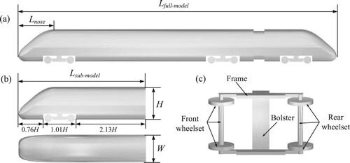
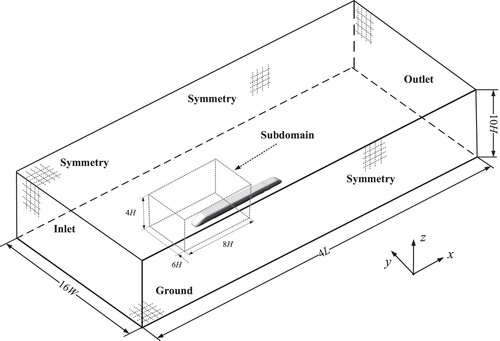
Since the research focuses on the aerodynamic noise of the leading car and the leading bogie, the middle of the leading car is truncated to create a sub-model, as shown in Figure 1(b). The length of the sub-model train is L_sub-model  = 14 m. The computational domains of the full model and the sub-model are shown in Figure 2. The computational domain size of the full model is 4L × 16W × 10H, which is larger than the minimum value of the train aerodynamic numerical simulation computational domain, and larger than the size selected by Li et al. (2019) in the study. Therefore, the computational domain size is sufficient to capture the details of the flow field around the train. In the current study, the computational domain size of the sub-model is 8H × 6H × 4H, which is relatively larger than the subdomain size used by Zhao et al. (2020) in their investigation of pantograph aerodynamic noise. Zhao et al. (2020) pointed out that the region of interest around the sub-model requires a highly refined mesh to achieve high-resolution simulation of the flow field and sound field. The sub-domain model exists inside the full model, and all input data come from the aerodynamic calculation of the full model. Therefore, depending on the accuracy of the full model flow field simulation, the influence of the boundary of the sub-model calculation domain on the simulation results will be controllable. For the full model, the front and rear surfaces of the computational domain are set as the velocity inlet and pressure outlet boundaries, respectively. The two sides and the top are set as symmetrical boundaries. The ground is a slip surface with the same velocity as the incoming flow. For the sub-model, the data of all boundaries of the computational domain are interpolated by the results obtained by the full model domain calculation. These data include velocity, turbulent kinetic energy and turbulent dissipation rate.

Figure 2. Computational domain of the full model and sub-model.

All subsequent computational cases are divided into two steps. First, perform aerodynamic calculations for the full model to obtain data information on the boundaries of the sub-model computation region. Then, based on the initial field boundary data, perform aerodynamic and acoustic calculations for the sub-model. Both the full model calculations and the preliminary steady calculations in this study were performed using the RANS turbulence model.

3.2. Case descriptions

Due to constraints imposed by wind tunnel construction and operating costs, it is still difficult to conduct full-scale model experiments of trains, thus only reduced-scale model experiments can be conducted. Meanwhile, although numerical simulations of aerodynamic noise for full-scale model trains are feasible, they still require significant computational resources and costs. Reducing the scale of the model and decreasing the inflow velocity of upstream turbulence can significantly reduce the grid requirements for acoustic calculations. Therefore, three different cases are simulated to investigate the effects of model scale (λ) and airflow velocity ratio (γ) on the aerodynamic noise of the high-speed train leading car and leading bogie.

The case descriptions are given in Table 2. Case0 is used as the baseline condition with a model scale of 1/1 and an actual inflow velocity of 400 km/h. For Case1, the inflow velocity remains unchanged but the model scale is reduced to 1/10. For Case2, both the model scale and the inflow velocity are simultaneously reduced to 1/10 of the baseline condition. It is worth noting that both case1 and case2 will lead to a decrease in Reynolds number, which will introduce a certain degree of error to the high-frequency noise information, while the bogie noise is mainly low-frequency, and its absolute noise level will not be significantly affected. Case1 ensures that the incoming flow velocity is constant, and the influence of the decrease of Reynolds number on the absolute noise level is within a certain range. The model scale and incoming flow velocity of case2 are both proportionally reduced to minimise the impact on the Strouhal number and achieve a flow field more similar to that of the full-scale model (He et al., 2024). The definitions of Mach number (Ma), Strouhal number (St), Reynolds number (Re) and dimensionless wall distance y+ are as follows: (1) $\begin{array}{rl}\mathrm{Ma}& =\frac{U_{\mathrm{\infty }}}{c}\end{array}$(1) (2) $\begin{array}{rl}\mathrm{St}& =\frac{\mathrm{fH}}{U_{\mathrm{\infty }}}\end{array}$(2) (3) $\begin{array}{rl}\text{Re}& =\frac{U_{\mathrm{\infty }}H}{\nu }\end{array}$(3) (4) $\begin{array}{rl}{\text{y}}^{+}& =\frac{y{u}_{\tau }}{\nu }\end{array}$(4)

Table 2. Case descriptions.

Case	λ	U∞ (km/h)	Ma	St	Re
Case0	1/1	400	0.326	0.032f	2.7 × 10^7
Case1	1/10	400	0.326	0.0032f	2.7 × 10^6
Case2	1/10	40	0.0326	0.032f	2.7 × 10^5

Where U_∞ is the airflow velocity, H is the train height as the model characteristic scale, c represents the speed of sound with a value of 340 m/s, f represents the fluid oscillation frequency, v is the kinematic viscosity, y is the distance from the wall to the first cell centre, u_τ is the friction velocity.

3.3. Grid strategy

For acoustic simulation, the quality of the grid will directly affect the accuracy of the simulation results. The grid should have sufficient resolution to capture the detailed structure of the flow field, especially the turbulence results generated in high-speed flow. In the aerodynamic calculation of the full model, relatively large-scale train surface and boundary layer grids can be set up to obtain the boundary data of the sub-model calculation domain. In contrast, very fine meshes are required for aerodynamic and noise calculations of sub-models.

To eliminate the influence of grid uncertainty on the results, three sets of grids were selected to test the simulation accuracy for case0 conditions. The same grid scale was used for calculations of the full model to obtain consistent data at the boundaries of the subdomains. However, the discretization grid scale gradually decreased within the subdomains. Additionally, to simulate wall flows, all three grid sets created boundary layer grids with a total of 25 layers and a grid growth ratio of 1.1. These grids ensured that the wall non-dimensional distance y+ was less than 1, and the distribution of y+ values on the medium grids is shown in Figure 3. To evaluate the prediction accuracy of the three grid sets for far-field noise, 15 microphones were placed at a distance of 25 m from the high-speed train and 3.5 m above the ground to obtain sound pressure data. The spacing between the microphones was 3 m, as shown in Figure 4. For reduced scale cases, the receiver distance is scaled proportionally to the model scale to maintain geometric similarity. This ensures that the aerodynamic noise similarity is preserved, with minimal impact on the far-field sound pressure level (SPL) due to the consistent scaling of both the model and the receiver distance (Li et al., 2022a). Using the entire sub-model as the noise source, the maximum sound pressure level (max SPL, reference sound pressure P_ref= 2 × 10⁻⁵Pa) and the average sound pressure level (avg SPL) of all 15 receivers were compared, and the results are listed in Table 3. Compared to the fine grid, the difference of the medium grid is less than 0.5 dB, while the difference of the coarse grid is close to 1 dB. The velocity and pressure distributions are obtained by solving the flow field based on the RANS model. The broadband noise source model is then used to estimate the noise source strength from the flow field data and subsequently calculate the surface sound power (P_W). P_W represents the sound power per unit area caused by turbulence, reflecting the noise intensity at various points on the surface. The surface sound power level (L_W) is the logarithmic representation of surface sound power, indicating the aerodynamic noise power per unit area on the train surface, measured in decibels (dB). Similar to the definition of sound pressure level, $L_W=10{\log }_{10}(P_W/P_0)$, P₀ is the reference sound power, valued at 1 × 10⁻¹² W. Figure 5 shows the prediction results of L_W on the train surface at three grid densities. The prediction results of the three sets of grids in the upper surface area of the high-speed train are basically consistent, while the prediction results on the surface of the bogie cavity are different to some extent. The difference between medium and fine grids is smaller. Therefore, overall evaluation suggests that the medium grid is more suitable for subsequent numerical simulation studies. Figure 6 shows the final grid results of the sub-model. The total grid count is approximately 37.14 million, with a grid size of 0.24 m. Three refinement zones were created around the sub-model train for grid transition, and the minimum grid size on the train surface ranges from 15 to 30 mm.

Figure 3. Distribution of surface y+ values based on the full model of case0.

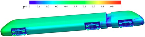
Figure 4. Position diagram of acoustic receivers (case0).

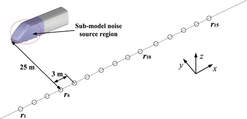
Figure 5. Comparison of acoustic results of train surface under different mesh densities.

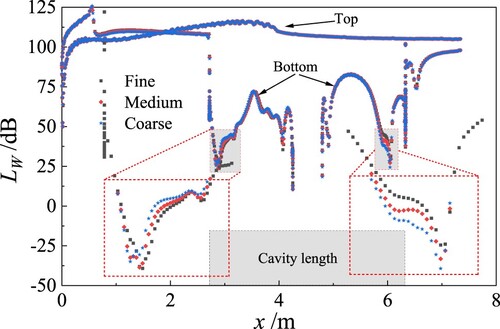
Figure 6. Distribution of grids on and around the train surface.

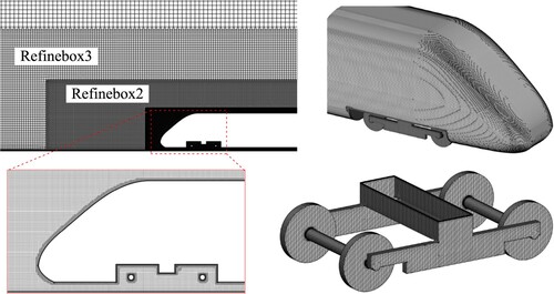
Table 3. Comparison of far-field noise results under different grid densities.

	Base		Grid
	size/m		number/million
	Full	Sub-	Full	Sub-	Max	Avg
Mesh	model	model	model	model	SPL/dB	SPL/dB
Fine	0.96	0.16	47.65	46.52	97.7	96.4
Medium		0.24		37.14	98.0	96.8
Coarse		0.32		29.47	98.5	97.3

Case1 and case2 both involve scaling down the model based on case0. Therefore, the grids for both the full model and the sub-model in case1 and case2 are directly scaled from case0, which also meets the requirement that the wall non-dimensional distance y+ value of the wall is less than 1. However, this grid strategy inevitably causes differences in grid resolution and y+ values. Considering that it is challenging to ensure the same y+ values across three sets of grids even if the boundary layer grid dimensions are defined individually for each case, it is crucial to ensure that the dimensionless y+ value is less than 1 in all cases to achieve sufficient resolution of the boundary layer. Li et al. (2022a) used a similar grid division strategy in their study, and the numerical results were validated by wind tunnel experiments, indirectly demonstrating the feasibility of this method.

3.4. Numerical settings

The same solution strategy is adopted for the current three simulation cases. Firstly, aerodynamic calculations are performed for the full model train, with the turbulent model selected as the SST k-ω model to ensure the flow field is fully developed. Subsequently, the flow field physical quantities on the boundaries of the subdomain are extracted as input data. Secondly, steady calculations are conducted for the flow field around the sub-model train. Then, based on the IDDES turbulence model, the unsteady flow field of the sub-model train is calculated, and the sound source data is extracted after the flow field stabilises. Finally, far-field radiated noise is calculated using the sound source data as the input for the sound source term of the FW-H equation.

During the simulation process, steady calculations serve as the initial values for the subsequent calculation steps. The time step for unsteady calculations is set to 5 × 10⁻⁵s, ensuring that the acoustic Courant–Friedrichs-Lewy number ($\mathrm{CFL}=c\mathrm{\Delta t}/\mathrm{\Delta x}$, $\mathrm{\Delta }t$ is the time step, $\mathrm{\Delta }x$ is the spatial step) is less than 1 for all cases. The total simulation time of unsteady calculation is 0.4 s, and the time of collecting the fluctuating pressure on the surface of the train as the sound source term of the FW-H equation is 0.2 s. The turbulence models, turbulence quantities and spatial discretization schemes used in the numerical simulation of the whole process are listed in Table 4.

Table 4. Solver settings for numerical simulation.

	Full-model	Sub-model
Simulation process	Steady simulation	Steady simulation	Unsteady simulation
Turbulent model	SST k-ω	SST k-ω	IDDES
Solver Type	Pressure-Based	Pressure-Based	Pressure-Based
Solution Methods	SIMPLE	SIMPLE	SIMPLE
Gradient	Least Squares Cell Based	Least Squares Cell Based	Least Squares Cell Based
Spatial Discretization	Second Order Upwind	Second Order Upwind	Bounded Central Differencing
Turbulent quantities	Second Order Upwind	Second Order Upwind	Second Order Upwind
Time Formulation	/	/	Second Order Implicit
Time step	/	/	CFL < 1

4. Validation

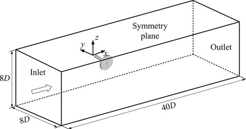
To validate whether the mesh scale and turbulence model used in the current study can accurately capture flow features related to aerodynamic noise, it is necessary to compare simulation results with experimental data from actual cases. However, due to the lack of wind tunnel experiments for complex bogies, we chose to evaluate our methods using experimental data of aerodynamic noise from simple bogies available in the literature. Given the similarity in noise generation mechanisms between simple wheelsets and complex bogies, these results can be used to assess the effectiveness of the numerical methods employed in the current study. In this paper, a case model identical to that of Zhu et al. (2014) was established. This model is half of a 1/10 scale isolated wheelset with a wheel diameter of D = 92 mm and an axle diameter of d = 17.5 mm. The computational domain is shown in Figure 7, with the coordinate origin located at the centre of the axle end face. The velocity and pressure outlet boundary conditions are applied to the upstream inlet surface and the downstream outlet surface, respectively. The inlet velocity is 30 m/s and the outlet pressure is 0 Pa. The wheel surface is set as a non-slip wall. All other surfaces are set as symmetric boundary conditions.

Figure 7. Isolated wheelset model for numerical validation.

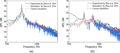
The details of the aerodynamic noise experiment related to this model can be found in Zhu et al. (2014). To evaluate the aerodynamic noise characteristics of the wheelset, two microphones were placed on the top and side of the wheelset. The coordinates are (−18, 1375, 31.3) mm and (0, 185, 2211.3) mm, respectively. The current simulation results are compared with the wind tunnel test and numerical simulation results of Zhu et al. (2014), as shown in Figure 8. Both the experimental measurements and the numerical simulation results are processed by the Welch method with the same frequency bandwidth (Δf = 6 Hz). This ensures consistency and prevents sound pressure level differences due to different frequency resolutions. The numerical simulation and experiment show a high degree of consistency in the noise spectrum of the acoustic receiver, although there are many differences in the sound pressure level. The current simulation, similar to that by Zhu et al. (2014), treats the truncation surface of the wheel axle end face as a symmetric plane. However, in wind tunnel experiments, this surface is a solid wall that reflects sound and increases the sound pressure level. Overall, the numerical simulations can accurately predict the frequency peaks of the tonal noise observed in the experimental measurements. This indicates that the grids and numerical simulation methods used in the current study are effective in predicting the noise characteristics of the wheelset.

Figure 8. Comparison of noise spectra for far-field acoustic receivers: (a) top receiver and (b) side receiver.

5. Results and discussions

5.1. Flow field

Figure 9 shows the distribution of the time-averaged pressure coefficient (c_p) in the longitudinal centre section of the train (y = 0) and in the flow field space beneath the train. The c_p is defined as follows: (5) $c_p=\overline{P}/\left(\frac{1}{2}\rho U_{\mathrm{\infty }}^2\right)$(5) Where $U_{\mathrm{\infty }}$ is the inflow velocity, $\overline{P}$ is the time-averaged pressure, and ρ is the density.

Figure 9. Time-averaged pressure distribution on the: (a) train surface and (b) train bottom.

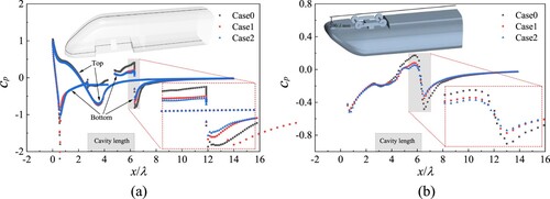
From Figure 9, all cases exhibit a consistent trend in pressure distribution. Lauterbach et al. (2012) investigated the aerodynamic noise of the ICE3 high-speed train bogie at Reynolds numbers of 4.6 × 10⁵ and 3.7 × 10⁶. The results of the two wind tunnel experiments showed a strong similarity. The Reynolds numbers in the current study are all above 10⁵, suggesting that the Reynolds numbers may be within the self-similarity zone, leading to similar dynamic behaviour and flow structures in the flow field. However, there are also differences in local regions. As depicted in Figure 9(a), the pressure distribution on the upper surface of the train is basically consistent, whereas significant variations are observed on the surface of the bogie cavity. Both case1 and case2 display lower pressure amplitudes compared to case0, which can be attributed to the reduction in model scale. Reducing the scale of the bogie model increases the local viscous flow, resulting in a decrease in the regional flow velocity, which weakens the absolute pressure level in the flow field to a certain extent. In addition, it can also be seen from Figure 9(b) that the flow field pressure amplitude of case0 in the bogie area is larger, indicating that case0 will generate a higher level of aerodynamic noise in this region.

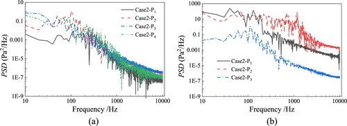
As shown in Figure 10, in order to further compare the differences in surface pressure fluctuations among different cases, four pressure monitoring points were arranged on the surface of the train bottom and the bogie surface. Figure 11(a) shows the power spectral density (PSD) of the four pressure monitoring points in case2. The pressure fluctuations on the upstream surface of the bogie cavity are lower than those on the surface of the bogie. The energy of fluctuating pressure is mainly concentrated in the frequency region below 400 Hz. In addition, the pressure fluctuation intensity on the front wheelset axle surface is higher, while the pressure fluctuation intensity on the bolster and rear wheelset axle surfaces is relatively similar. Figure 11(b) shows the comparison of PSD at the P₂ pressure monitoring point for different cases. It can be seen that the energy level of case0 is the highest, while case1 and case2 reduce the turbulent energy due to the decrease of model scale or incoming flow velocity. Compared to case0, case1 exhibits a different pattern primarily due to the frequency shift caused by the model scale, whereas case2 maintains the same Strouhal number and has a more similar energy distribution trend to case0.

Figure 10. Train surface monitoring point location diagram.

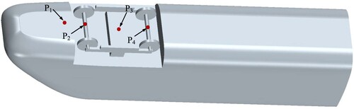
Figure 11. Spectrum characteristics of train surface pressure monitoring points: (a) Measurement points P₁–P₄ for case2, and (b) Measurement point P₂ for different cases.

In the flow field of the leading bogie under the train head, the noise source comes from the vortex motion of the fluid or the pressure fluctuation caused by the interaction between the fluid and the structural surface. By analysing the pressure and velocity distributions in the flow field and combining the acoustic theory, the positions and mechanisms of noise sources can be identified. The method based on the Q criterion is a visualisation method commonly used in the vortex structure of the train flow field, which identifies the vortex structure based on the velocity gradient of the flow field. The vortex region is usually accompanied by the interlacing of pressure gradient and velocity gradient. This interlacing reflects that the fluid rotates in these regions, thus forming a vortex. The Q criterion is defined as follows: (6) $\begin{array}{rl}Q& =1/2({\mathrm{\Omega }}_{{}_{\mathrm{ij}}}^2-S_{{}_{\mathrm{ij}}}^2)\end{array}$(6) (7) $\begin{array}{rl}{\mathrm{\Omega }}_{\mathrm{ij}}& =1/2(\mathrm{\partial }{u}_i/\mathrm{\partial }{x}_j-\mathrm{\partial }{u}_j/\mathrm{\partial }{x}_i)\end{array}$(7) (8) $\begin{array}{rl}{S}_{\mathrm{ij}}& =1/2(\mathrm{\partial }{u}_i/\mathrm{\partial }{x}_j+\mathrm{\partial }{u}_j/\mathrm{\partial }{x}_i)\end{array}$(8) (9) $\begin{array}{rl}\tilde{Q}& =Q{H}^2/U_{\mathrm{\infty }}^2\end{array}$(9)

Where ${\mathrm{\Omega }}_{\mathrm{ij}}$ and $S_{\mathrm{ij}}$ are vorticity tensor and strain rate tensor, respectively. $\tilde{Q}$ is normalised Q criterion.

Figure 12 shows the vortex structures inside the bogie cavity with different $\tilde{Q}$ values, coloured by velocity. As the airflow in front of the bogie reaches the leading edge of the cavity, it immediately separates and forms a highly complex turbulent wake inside the cavity. Bogie components located behind the separated shear layer jet hinder the further development of the wake. Meanwhile, airflow impinging on the surfaces of the bogie components regenerates vortex structures with high vorticity. The separated shear layer generates vortices due to Kelvin-Helmholtz instability. These vortex structures dissipate behind the bogie components, forming vortices of various scales, which exacerbates the complexity of the flow field. For all three cases, the topological structures of the vortex structures formed within the bogie region under different model scales and inflow velocities are similar, but significant differences exist in local regions. The generation and development of vortex structures are influenced by various factors, including fluid dynamics, structural geometric shapes, and airflow conditions. Compared to case0, reducing the model scale in case1 limits the development space of the flow field, resulting in a decrease in the number and scale of vortex structures. However, case2 exhibits vortex structures more similar to case0, possibly due to their similar vortex shedding frequencies. Overall, similar vortex structures are observed for all cases. Although both case1 and case2 significantly reduce the Reynolds number, this does not fundamentally change the turbulent nature of the shear layer jet itself, thereby maintaining the similarity in the formation of vortices within the airflow through rotation and mixing.

Figure 12. The instantaneous distribution of vortex structure in bogie region with different $\tilde{Q}$ values, coloured by velocity: (a) case0,(b) case1 and (c) case2.

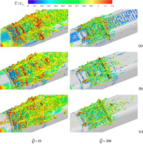
Figure 13 presents the instantaneous spanwise (ω_y) and vertical vorticity (ω_z) fields on the longitudinal central section (y = 0) and the vertical section (z = 0.18H). It can be seen that the vorticity field distribution of all cases is similar in the whole and different in the local. For case1 and case2, reducing the model scale localises the flow field around the bogie components, resulting in a more concentrated distribution of vorticity in the local area. At the same time, the decrease of model scale also leads to the increase of shear layer thickness, which in turn affects the formation and distribution of vorticity field. In addition, for case2, the decrease of the flow velocity will lead to the weakening of the power required for the generation and maintenance of the vortex in the flow field.

Figure 13. The instantaneous vorticity field distribution on the longitudinal central section (y = 0) and the vertical section (z = 0.18H): (a) case0, (b) case1 and (c) case2.

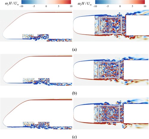
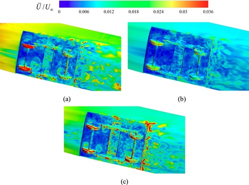
Figure 14 further shows the comparison of dimensionless time-averaged velocity ($c_u=\overline{U}/U_{\mathrm{\infty }}$, $\overline{U}$ is the time-averaged velocity) and time-averaged vorticity magnitude ($\mathrm{\varpi H}/U_{\mathrm{\infty }}$) in the flow field space at the bottom of the train. The airflow velocity and vorticity distribution at the bottom of the train are basically similar in the three cases, and the main differences are reflected in the bogie area and downstream of the cavity. Figure 14(a) shows that due to the reduction in model scale, the flow velocity beneath the bogie area increases in both case1 and case2, while the relative flow velocity at the rear edge of the cavity is greater in case0. From Figure 14(b), it can be seen that in case1, the reduction in model scale results in a decrease in the time-averaged vorticity magnitude in both the bogie cavity region and the downstream region. A similar result can be observed in case2, but the reduction is less pronounced. Overall, the flow field distribution beneath the train in case2 is closer to that in case0.

Figure 14. Comparison of flow field at the bottom of train: (a) dimensionless time-averaged velocity and (b) time-averaged vorticity magnitude.

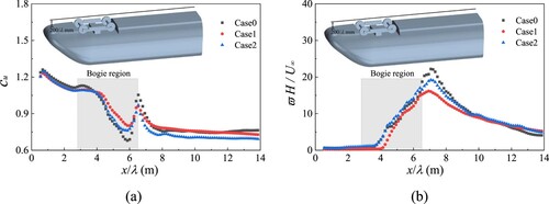
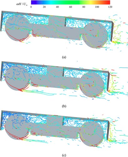
Figure 15 shows the vortex core distribution in the bogie region. There are numerous vortex structures within the bogie cavity. The weak vorticity and small-scale vortex are mainly distributed in the space between the cavity and the bogie components, while the strong vorticity and large-scale vortex are mainly distributed around the front wheelset, rear wheelset, and the rear edge of the cavity. It is worth noting that the vortex shedding from the bottom of the front wheelset has the longest drag distance and higher vorticity. For case1 and case2, the vortex drag distance at the bottom of the front wheelset is longer. The decrease in model scale results in the airflow development distance being relatively farther. However, reducing the model scale leads to smaller vortex core scales and weaker intensity of the vortex cores, especially in the region between the cavity and the bogie.

Figure 15. The instantaneous vortex core distribution in the bogie region: (a) case0, (b) case1 and (c) case2.

5.2. Aerodynamic noise source

The dipole noise in the bogie region mainly comes from the turbulent pressure fluctuation caused by the irregular movement of the fluid near the wall. The Curle equation can be used to analyse the aerodynamic noise caused by the solid surface (Curle, 1955). The total sound power level of the solid surface radiation can be approximately expressed as: (10) $W={\int }_{S}I(\mathbf{\text{y}})\mathrm{dS}(\mathbf{\text{y}})={\int }_S\frac{A_c(\mathbf{\text{y}})}{12{\rho }_0\pi c_0^3}\overline{{\left[\frac{\mathrm{\partial }p}{\mathrm{\partial }t}\right]}^2}\mathrm{dS}(\mathbf{\text{y}})$(10) Where $I(\mathbf{\text{y}})$ is the noise contribution per unit area to the total sound power, that is, the sound intensity, and S is the surface area of the solid sound source. y denotes the point on the surface of the sound source. $A_c(\mathbf{\text{y}})$ is the correlation area of point y, and the surface pressure fluctuation of any point in this area is related to point y. In general, the turbulent pressure fluctuation propagates with the local convective velocity of the fluid. Therefore, the correlation region, the characteristic length scale $l_c(\mathbf{\text{y}})$ and the local mean convection velocity ${\overline{U}}_c(\mathbf{\text{y}})$ at the y-point sound source have the following relationship (Phan et al., 2017): (11) $A_c(\mathbf{\text{y}})\propto l_c^2(\mathbf{\text{y}})\propto {\overline{U}}_c^2(\mathbf{\text{y}})$(11) It can be seen from Equation (11) that the external noise power of the solid surface is related to the time derivative $\mathrm{\partial }p/\mathrm{\partial t}$ of the surface pressure fluctuation and the local mean convection velocity ${\overline{U}}_c(\mathbf{\text{y}})$. In addition, it is generally assumed that the ratio of the local convection velocity to the airflow velocity is constant. Therefore, the time-averaged velocity of the near-wall surface airflow can be used to approximate the correlation region on the sound source surface.

To compare the effects of different model scales and turbulent inflow conditions on the sound source distribution. The root mean square value ($c_{p,\mathrm{rms}}^{\mathrm{\prime }}$) of the time derivative of the pressure coefficient is defined to evaluate the sound source intensity characteristics of the three cases. $c_{p,\mathrm{rms}}^{\mathrm{\prime }}$ is defined as follows: (12) $c_{p,\mathrm{rms}}^{\mathrm{\prime }}=\sqrt{\frac{{\int }_{t_1}^{t_2}({c^{\mathrm{\prime }}}_p{)}^2\mathrm{dt}}{T}}$(12) Where $c_p^{\mathrm{\prime }}=d{c}_p/d{t}^{\ast }$ is the time derivative of the pressure coefficient, $t^{\ast }=\mathrm{tU}/H$ is the dimensionless time, and T is the extraction time of the source data.

Figures 16 and 17 show the surface pressure fluctuation and the average velocity distribution of the near-wall surface in the bogie area, respectively. In Figure 16, for all cases, high surface pressure fluctuation regions can be found on the frame, rear wheelset, rear end face of the cavity and downstream surface of the cavity. However, in Figure 17, the high average speed region appears in the front wheelset, the rear wheelset and the rear edge of the cavity. According to Equation (10), when the high surface pressure fluctuation region and the high average velocity region overlap, a large noise power will be generated. Therefore, the rear wheelset, the rear edge of the cavity and the downstream surface will be the most important sound source components in the bogie region.

Figure 16. Surface pressure fluctuation distribution in the bogie region: (a) case0, (b) case1 and (c) case2.

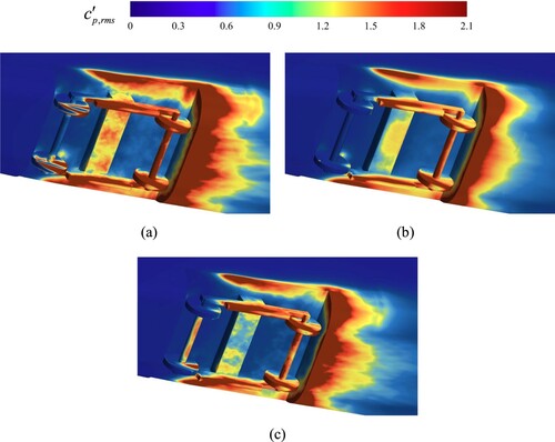
Figure 17. Mean velocity distribution near the wall of the bogie region: (a) case0, (b) case1 and (c) case2.

From Figure 16, it can be seen that the surface pressure fluctuation distribution in the three cases is similar overall. Compared to case0, case1 exhibits a reduction in the intensity of pressure fluctuations on the bolster, the upper surface of the cavity, the trailing edge of the cavity, and the downstream surface. At the same inflow velocity, a decrease in model scale leads to a reduction in Reynolds number and changes in local vortex structures. The decrease in vortex energy will reduce turbulent excitation on the solid surface, resulting in a decrease in the magnitude of surface fluctuating pressure. The consistency of case2 and case0 in Strouhal numbers may indicate similarities in the distribution of turbulent energy and the scales of turbulence relative to the fundamental flow characteristics in both cases. Therefore, the distribution of surface pressure fluctuations induced by flow in the two case models is more similar.

From Figure 17, it can be seen that the near-wall time-averaged velocity distribution of case2 and case0 is similar, and case1 shows a lower near-wall velocity level as a whole. Chang et al. (2022) investigated the scale effect of the high-speed train model, and pointed out that as the model scale decreases, the relative boundary layer thickness on the train surface increases, which indicates that the near-wall velocity gradient decreases. Therefore, the significant differences observed in case1 are mainly attributed to the reduction of the model scale, which largely limits the airflow under the train, resulting in different flow patterns and velocity distributions compared with other cases. However, case2 and case1 have different conditions. The decrease of the inflow velocity makes the Strouhal number maintain a similar state in case0, and the flow distribution near the wall is more similar. It is expected that the airflow at the bottom of the train should show more similarity with case0. In case2, it can be observed that the relative velocity near the wall at the rear edge of the cavity is larger. Even if the Strouhal number is similar, the decrease of the model scale leads to the change of the physical scale of the space at the bottom of the train, which will also lead to some differences in the flow separation position and velocity gradient distribution in the key area of the bogie cavity.

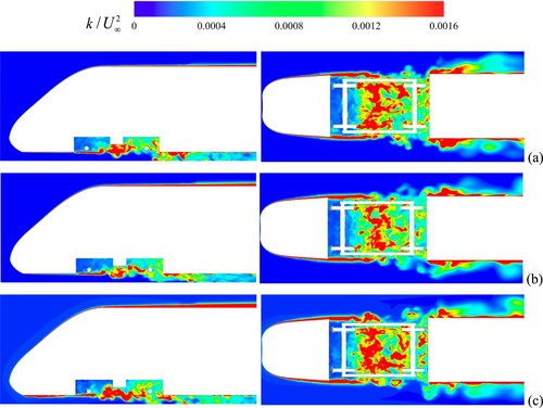
Vortices in turbulent flow can generate large velocity and pressure fluctuations and become aerodynamic sound sources. By analyzing the spatial distribution of turbulent kinetic energy ($k=0.5(u^{\mathrm{\prime }2}+v^{\mathrm{\prime }2}+w^{\mathrm{\prime }2})$, where $u^{\mathrm{\prime }}$, $v^{\mathrm{\prime }}$ and $w^{\mathrm{\prime }}$ are the components of velocity fluctuation in x, y and z directions), the position and intensity of the vortex structure can be inferred to locate the aerodynamic sound source. Figure 18 shows the instantaneous turbulent kinetic energy distribution on the longitudinal central section (y = 0) and the vertical section (z = 0.18H). It can be seen that a jet shear layer is formed at the front and two sides of the bogie cavity, and the airflow continuously falls off during the downstream movement to form a vortex acting on the bogie structure. The high turbulent kinetic energy region is concentrated in the centre of the bogie structure and downstream of the cavity. It can be seen that there is a strong vortex interaction in these regions. The separated shear layer airflow generates a large unsteady flow on the bolster, rear wheelset and rear end surface of the cavity, indicating that the surface of these components may generate large pressure fluctuations. Comparing the three different cases, case0 and case2 show more similar turbulent kinetic energy distribution, especially in the middle and rear areas of the bogie, because the vortex shedding frequency is closer. However, the relative turbulent kinetic energy levels near the bottom of the cowcatcher upstream of the bogie are higher. The reason may be that the reduction in model scale changes the boundary layer structure and decreases the gap height, leading to enhanced interaction between the train wake and the ground. Additionally, relative turbulent kinetic energy levels correlate with inflow velocity, and the lower inflow velocity may result in higher turbulent kinetic energy levels in the cowcatcher region.

Figure 18. The instantaneous turbulent kinetic energy distribution around the train: (a) case0, (b) case1 and (c) case2.

5.3. Far-field noise

Figure 4 shows the locations of the full-scale train far-field acoustic receivers used to quantify the magnitude of the far-field noise. To investigate the radiated noise from each component of the noise source, the train is divided into several independent noise sources. As shown in Figure 19, the noise sources of a high-speed train are divided into car body, cavity, and bogie, with the bogie further divided into front wheelset, rear wheelset, frame, and bolster.

Figure 19. Division of sound source components.

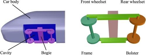
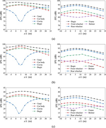
Figure 20 shows the overall sound pressure level (OASPL) of different independent sound source components at the receivers. It can be seen that for the leading car of the high-speed train, the streamlined car body and the bogie are the most significant sound source components. The overall noise level of the bogie cavity is relatively low, but its impact on the downstream area is more significant. In addition, for bogie noise, the rear wheelset is the primary noise source. In terms of relative contribution, the three different cases show similar results. However, some differences can also be observed. For case0, the noise level of the bogie is higher than that of the car body, while the opposite result is obtained in case1 and case2. This difference is mainly attributed to changes in local viscous flow in the bogie region due to the decrease in model scale and airflow velocity. In case1 and case2, another difference is also reflected in the contribution level of each component of the bogie, such as the ranking of noise contributions from the front wheelset, frame, and bolster. Overall, the reduction in Reynolds number does not significantly affect the main noise source components such as the car body, bogie, or rear wheelset.

Figure 20. OASPL comparison of different components as noise sources: (a) case0, (b) case1 and (c) case2.

It can be seen from Figure 20 that in case2, the absolute noise level is significantly lower than the other two cases. For Equation (10), the order of magnitude of the surface pressure fluctuating is converted to the average velocity: (13) $\overline{{\left[\frac{\mathrm{\partial }p}{\mathrm{\partial }t}\right]}^2}\propto {\overline{U}}_c^4(\mathbf{\text{y}})$(13) Furthermore, the relationship between the sound intensity generated by solid surface motion and velocity is sixth power, as follows: (14) $I\propto {\overline{U}}_c^6(\mathbf{\text{y}})$(14) In summary, the relationship between the sound intensity and the characteristic length (l), airflow velocity (U_∞), and distance (r) from the sound receiver is as follows (Curle, 1955): (15) $I\propto \frac{U_{\mathrm{\infty }}^6{l}^2}{r^2}$(15) For simulation cases with different model scales and airflow velocities, the conversion relationship between sound pressure levels is as follows: (16) $\begin{array}{rl}\mathrm{\Delta }\mathrm{SPL}& =10{\log }_{10}\left[{\left(\frac{U_{\mathrm{\infty },1}}{U_{\mathrm{\infty },2}}\right)}^6{\left(\frac{l_1}{l_2}\right)}^2{\left(\frac{r_2}{r_1}\right)}^2\right]\\ & =10{\log }_{10}({\gamma }^6{\lambda }^2{R}^{-2})\end{array}$(16) Where $\mathrm{\Delta }\mathrm{SPL}$ represents the difference in sound pressure levels between two different simulation cases. γ = U_∞,1/U_∞,2 is the ratio of airflow velocities, λ = D₁/D₂ is the ratio of model scales, and R = r₁/r₂ is the ratio of distances from the sound source to the sound receiver. Because the arrangement position of the acoustic receiver is equally scaled according to the model scale. Therefore, case0 and case1 should have comparable noise levels. This can be verified from Figure 20(a and b). However, for case2, due to the decrease of the incoming flow velocity, the sound pressure level will decrease by $60{\log }_{10}(\gamma )$, that is, 60 dB, as shown in Figure 20(c).

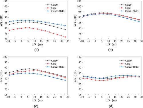
Figure 21 shows a comparison of the far-field noise results for the three cases. For case2, 60 dB is added to the sound pressure level at all receivers to obtain the corresponding sound pressure level at full speed. It can be seen that the sound pressure levels of the three simulation cases are comparable for the cavity and bogie components. However, for the car body, case1 and case2 show different degrees of difference, indicating that the similarity of the car body is weaker than that of the bogie region. Li et al. (2022a) also pointed out in their study that the differences in the noise levels generated by the car body of high-speed trains with different model scales are relatively large. In terms of the trend of far-field noise variation, case2 is closer to case0.

Figure 21. Comparison of OASPL results in different cases: (a) total, (b) car body, (c) cavity and (d) bogie.

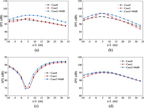
Figure 22 further illustrates the sound pressure levels generated by each component of the bogie. It can be seen that, for different cases, the largest differences in noise levels occur in the front wheelset, followed by the frame. The differences in noise levels for the bolster and the rear wheelset are relatively small. The jet shear layers generated at the bottom and both sides of the front edge of the cavity directly affect the front wheelset and frame. The reduction in model scale and inflow velocity will affect the jet shear layers to some extent, resulting in differences in noise levels for the front wheelset and frame. However, since the bogie noise comes mainly from the rear wheelset, the bogie noise levels are comparable in the three cases.

Figure 22. OASPL comparison for each component of the bogie: (a) front wheelset, (b) rear wheelset, (c) frame and (d) bolster.

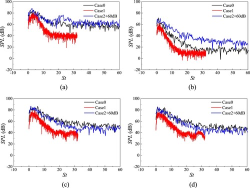
The model scale and inflow velocity directly affect the shedding frequency of vortices. The frequency scaling for the three cases satisfies the following equation: (17) $\frac{f_1}{f_2}=\left(\frac{U_{\mathrm{\infty },1}}{U_{\mathrm{\infty },2}}\right)\times \left(\frac{D_1}{D_2}\right)$(17) From Figure 20, it can be seen that the maximum sound pressure level is at receiver r₅ or r₆. Receiver r₆ is chosen for comparing the noise spectra. The Welch method is employed to determine the spectrum of the sound pressure signal, using a Hanning window as the window function with a 50% overlap factor, and each signal segment lasts approximately 0.1s. According to the Strouhal number, the frequency domain of all three cases is adjusted to the full-scale train model with a speed of 400 km/h. Figure 23 shows the noise spectra of receiver r₆. Case0 and case2 exhibit more similar frequency domain distributions, with only a 60 dB difference in absolute sound pressure level. This is because these two cases ensure approximately equal Strouhal numbers. In case1, the decrease of model scale leads to frequency shift. However, the overall trend remains consistent. For all three cases, the similarity of the noise spectra in the frequency domain gradually decreases for the rear wheelset, bogie, car body, and cavity.

Figure 23. Comparison of noise spectra at receiver r₆, with a frequency resolution of 10 Hz: (a) car body, (b) cavity, (c) bogie and (d) rear wheelset.

6. Conclusions

This paper simulates the aerodynamic noise generated by the leading car and front leading bogie of a high-speed train under different model scales and turbulent inflow velocities using the IDDES method and FW-H equation. The method has been validated with experimental data. The main conclusions are as follows:

1. For all cases, the flow field is likely in the self-similarity zone, with similar flow characteristics in the bogie area, though local differences exist. Reducing the model scale affects flow separation and surface velocity gradient distribution in the bogie area. In case1, reducing the model scale alone decreases flow velocity and pressure gradient due to increased local viscous flow. Although the vortex topology is similar, the intensity and scale of local vortices differ. In case2, maintaining a similar Strouhal number to case0 results in a more similar flow field distribution.

2. The rear wheelset, rear edge of the cavity, and downstream surface are the main noise sources. The jet shear layer and unsteady flow in the bogie areas induce aerodynamic noise. The distribution of pressure fluctuations on the bogie surface is generally similar across cases. In case1, reducing the model scale decreases surface pressure fluctuations. Case2, with an equal Strouhal number to case0, achieves a closer distribution of surface pressure fluctuations.

3. Far-field noise distribution patterns are similar for all cases. Case1 shows a noise level reduction after scale reduction. In case2, reducing both the model scale and inflow velocity results in an absolute noise level reduction of approximately 60 dB. The main sound source components remain unchanged, but there are frequency shifts in case1 and absolute sound pressure level corrections needed for case2.

In summary, reducing only the model scale can achieve approximately equivalent noise levels but with frequency domain differences. Reducing both the model scale and inflow velocity ensures similar frequency distributions but may result in absolute sound pressure level errors. Corrections based on model scale and inflow velocity are necessary for accurate acoustic performance reflections in numerical simulations or wind tunnel tests. These results provide a reference for scaled-down model tests or simulations to evaluate the aerodynamic performance of actual high-speed trains.

Data availability

The data that support the findings of this study are available from the corresponding author upon reasonable request.

Disclosure statement

No potential conflict of interest was reported by the author(s).

Additional information

Funding

This work was supported by National Natural Science Foundation of China (12372049, 52072319), Fundamental Research Funds for the Central Universities (2682023ZTPY036) and Independent Project of State Key Laboratory of Rail Transit Vehicle System (2023TPL-T06).

References

- Baker, C. J., & Brockie, N. J. (1991). Wind tunnel tests to obtain train aerodynamic drag coefficients: Reynolds number and ground simulation effects. Journal of Wind Engineering and Industrial Aerodynamics, 38(1), 23–28. https://doi.org/10.1016/0167-6105(91)90024-Q
- Chang, C., Li, T., Qin, D., & Zhang, J. Y. (2022). On the Scale size of the aerodynamic characteristics of a high-speed train. Journal of Applied Fluid Mechanics, 15(1), 209–220.
- Curle, N. (1955). The influence of solid boundaries upon aerodynamic sound. Proceedings of the Royal Society of London. Series A, Mathematical and Physical Sciences, 231(1187), 505–514.
- Dong, T. Y., Liang, X. F., Krajnovic, S., Xiong, X. H., & Zhou, W. (2019). Effects of simplifying train bogies on surrounding flow and aerodynamic forces. Journal of Wind Engineering and Industrial Aerodynamics: The Journal of the International Association for Wind Engineering, 191, 170–182. https://doi.org/10.1016/j.jweia.2019.06.006
- Ffowcs-Williams, J. E., & Hawkings, D. L. (1969). Sound generation by turbulence and surfaces in arbitrary motion. Philosophical Transactions for the Royal Society of London. Series A, Mathematical and Physical Sciences, 264(1151), 321–342.
- Guo, Z., Liu, T., Xia, Y., & Liu, Z. (2022). Aerodynamic influence of the clearance under the cowcatcher of a high-speed train. Journal of Wind Engineering and Industrial Aerodynamics, 220, 104844. https://doi.org/10.1016/j.jweia.2021.104844
- Han, Y. D., & Yao, S. (2017). Scale effect analysis in aerodynamic performance of high-speed train. Journal of Zhejiang University (Engineering Science), 51(12), 2383–2391.
- He, Y., Thompson, D., & Hu, Z. W. (2024). Aerodynamic noise from a high-speed train bogie with complex geometry under a leading car. Journal of Wind Engineering and Industrial Aerodynamics, 244, 105617. https://doi.org/10.1016/j.jweia.2023.105617
- Lan, J., & Han, J. (2017). Research on the radiation characteristics of aerodynamic noises of a simplified bogie of the high-speed train. Journal of Vibroengineering, 19(3), 2280–2293. https://doi.org/10.21595/jve.2017.18229
- Lauterbach, A., Ehrenfried, K., Loose, S., & Wagner, C. (2012). Microphone array wind tunnel measurements of Reynolds number effects in high-speed train aeroacoustics. International Journal of Aeroacoustics, 11(3–4), 411–446. https://doi.org/10.1260/1475-472X.11.3-4.411
- Li, Z. M., Li, Q. L., & Yang, Z. G. (2022b). Flow structure and far-field noise of high-speed train under ballast track. Journal of Wind Engineering and Industrial Aerodynamics, 220, 104858. https://doi.org/10.1016/j.jweia.2021.104858
- Li, T., Qin, D., & Zhang, J. Y. (2019). Effect of RANS turbulence model on aerodynamic behavior of trains in crosswind. Chinese Journal of Mechanical Engineering, 32(1), 85. https://doi.org/10.1186/s10033-019-0402-2
- Li, T., Qin, D., Zhou, N., Zhang, J. Y., & Zhang, W. H. (2022a). Numerical study on the aerodynamic and acoustic scale effects for high-speed train body and pantograph. Applied Acoustics, 196, 108886. https://doi.org/10.1016/j.apacoust.2022.108886
- Liang, X. F., Liu, H. F., Dong, T. Y., Yang, Z. G., & Tan, X. M. (2020). Aerodynamic noise characteristics of high-speed train foremost bogie section. Journal of Central South University, 27(6), 1802–1813. https://doi.org/10.1007/s11771-020-4409-8
- Lighthill, M. J. (1952). On sound generated aerodynamically. I. General theory. Proceedings of the Royal Society of London. Series A, Mathematical and Physical Sciences, 211(1107), 564–587.
- Liu, H. K., Chen, R. R., Zhou, S. Q., Gao, Y. P, Zou, Y., Liu, T. H., & Zhao, Y. T. (2023). Numerical study on the effect of pantograph fairing on aerodynamic performance at various train heights. Engineering Applications of Computational Fluid Mechanics, 17(1), 2261521. https://doi.org/10.1080/19942060.2023.2261521
- Liu, X. W., Zhang, J., Thompson, D., Iglesias, E. L., Squicciarini, G., Hu, Z. W., Toward, M., & Lurcock, D. (2021). Aerodynamic noise of high-speed train pantographs: Comparisons between field measurements and an updated component-based prediction model. Applied Acoustics, 175, 107791. https://doi.org/10.1016/j.apacoust.2020.107791
- Menter, F. R., Kuntz, M., & Langtry, R. (2003). Ten years of industrial experience with the SST turbulence model. Turbulence, Heat and Mass Transfer, 4(1), 625–632.
- Minelli, G., Yao, H. D., Andersson, N., Höstmad, P., Forssén, J., & Krajnovic, S. (2020). An aeroacoustic study of the flow surrounding the front of a simplified ICE3 high-speed train model. Applied Acoustics, 160, 107125. https://doi.org/10.1016/j.apacoust.2019.107125
- Nagakura, K. (2006). Localization of aerodynamic noise sources of Shinkansen trains. Journal of Sound and Vibration, 293(3), 547–556. https://doi.org/10.1016/j.jsv.2005.08.043
- Niu, J. Q., Liang, X. F., Zhou, D., & Liu, F. (2016). Reynolds number effect of unsteady aerodynamic force and spectrum characteristics of high-speed train. Journal of South China University of Technollogy (Natural Science Edition), 44(8), 82–90.
- Orellano, A., & Schober, M. (2006). Aerodynamic performance of a typical highspeed train. In Proceedings of the 4th WSEAS International Conference on Fluid Mechanics and Aerodynamics (pp. 18–25). Elounda, Greece.
- Phan, V. L., Tanaka, H., Nagatani, T., Wakamatsu, M., & Yasuki, T. (2017). A CFD analysis method for prediction of vehicle exterior wind noise. SAE International Journal of Passenger Cars-Mechanical Systems, 10(1), 286–299. https://doi.org/10.4271/2017-01-1539
- Qin, D., Li, T., Zhang, J. Y., & Zhou, N. (2023). Numerical study on aerodynamic drag and noise of high-speed pantograph by introducing spanwise waviness. Engineering Applications of Computational Fluid Mechanics, 17(1), 2260463. https://doi.org/10.1080/19942060.2023.2260463
- Qin, D., Li, T., Zhou, N., & Zhang, J. Y. (2024). Aerodynamic drag and noise reduction of a pantograph of high-speed trains with a novel cavity structure. Physics of Fluids, 36(2), 027108. https://doi.org/10.1063/5.0188831
- Shi, F. C., Shi, F. S., Tian, X. D., & Wang, T. T. (2022). Numerical Study on Aerodynamic Noise Reduction of Pantograph. Applied Sciences, 12(21), 10720. https://doi.org/10.3390/app122110720
- Shi, J. W., & Zhang, J. Y. (2024). Effect of bogie cavity endwall inclination on flow field and aerodynamic noise in the bogie region of high-speed trains. Computer Modeling in Engineering & Sciences, 139(2), 2175–2195. https://doi.org/10.32604/cmes.2023.043539
- Shur, M. L., Spalart, P. R., Strelets, M. K., & Travin, A. (2008). A hybrid RANS-LES approach with delayed-DES and wall-modelled LES capabilities. International Journal of Heat and Fluid Flow, 29(6), 1638–1649. https://doi.org/10.1016/j.ijheatfluidflow.2008.07.001
- Sima, M., Gurr, A. A., Orellano, A., & Mainline, B. (2008). Validation of CFD for the flow under a train with 1:7 scale wind tunnel measurements. In Proceedings of the BBAA VI International Colloquium on Bluff Bodies Aerodynamics and Applications.
- Spalart, P. R., Deck, S., Shur, M. L., Squires, K. D., Strelets, M. k., & Travin, A. (2006). A new version of detached eddy simulation, resistant to ambiguous grid densities. Theoretical and Computational Fluid Dynamics, 20(3), 181–195. https://doi.org/10.1007/s00162-006-0015-0
- Talotte, C., Gautier, P. E., Thompson, D. J., & Hanson, C. (2003). Identification, modelling and reduction potential of railway noise sources: A critical survey. Journal of Sound and Vibration, 267(3), 447–468. https://doi.org/10.1016/S0022-460X(03)00707-7
- Thompson, D. J., Iglesias, E. L., Liu, X. W., Zhu, J. Y., & Hu, Z. W. (2015). Recent developments in the prediction and control of aerodynamic noise from high-speed trains. International Journal of Rail Transportation, 3(3), 119–150. https://doi.org/10.1080/23248378.2015.1052996
- Tian, H. Q. (2019). Review of research on high-speed railway aerodynamics in China. Transportation Safety and Environment, 1(1), 1–21. https://doi.org/10.1093/tse/tdz014
- Zhao, Y. Y., Yang, Z. G., Li, Q. L., & Xia, C. (2020). Analysis of the near-field and far-field sound pressure generated by high-speed trains pantograph system. Applied Acoustics, 169, 107506. https://doi.org/10.1016/j.apacoust.2020.107506
- Zhu, C., Hemida, H., Flynn, D., Baker, C., Liang, X., & Zhou, D. (2017). Numerical simulation of the slipstream and aeroacoustic field around a high-speed train. Proceedings of the Institution of Mechanical Engineers Part F Journal of Rail and Rapid Transit, 231(6), 740–756. https://doi.org/10.1177/0954409716641150
- Zhu, J. Y., Hu, Z. W., & Thompson, D. J. (2014). Flow simulation and aerodynamic noise prediction for a high-speed train wheelset. Aeroacoustics, 13(7-8), 533–552. https://doi.org/10.1260/1475-472X.13.7-8.533
- Zhu, J. Y., Hu, Z. W., & Thompson, D. J. (2016). Flow behaviour and aeroacoustic characteristics of a simplified high-speed train bogie. Proceedings of the Institution of Mechanical Engineers Part F Journal of Rail and Rapid Transit, 230(7), 1642–1658. https://doi.org/10.1177/0954409715605129
- Zhu, J. Y., Hu, Z. W., & Thompson, D. J. (2018). The flow and flow-induced noise behaviour of a simplified high-speed train bogie in the cavity with and without a fairing. Proceedings of the Institution of Mechanical Engineers Part F Journal of Rail and Rapid Transit, 232(3), 759–773. https://doi.org/10.1177/0954409717691619