Efficient aerodynamic shape optimization by using unsupervised manifold learning to filter geometric features

Abstract

Many aerodynamic shape optimization methods often focus on utilizing the end-to-end relationship between design variables and aerodynamic performance to find the optimal design, while overlooking the exploration of geometric knowledge of the shape itself. To fully use geometric knowledge to improve optimization efficiency, this paper proposes an efficient method by exploring the potential correlation between geometric features and aerodynamic performance at a low cost. We use unsupervised isometric feature mapping in manifold learning to capture geometric features that can distinguish the aerodynamic performance of different airfoils without embedding any tags. Then a filter criterion is establish based on the geometric features. During the optimization process, airfoils that deliver poor aerodynamic performance can be filtered out with a high probability before being precisely evaluated through computational fluid dynamics simulations. This helps improve samples quality to enhance the optimization efficiency. We applied the proposed method to the unconstrained and constrained optimizations of the Royal Aircraft Establishment (RAE) 2822 airfoil to validate its performance. The results demonstrate that the proposed method can improve the efficiency of optimization by over 50% compared with the original evolutionary optimization algorithm. It performs well across various optimization problems, demonstrating high engineering practical value.

KEYWORDS:

• Aerodynamic shape optimization
• manifold learning
• isometric feature mapping
• geometric features
• correlation

1. Introduction

The technology for optimization that combines computational fluid dynamics (CFD) simulations with algorithms of numerical optimization is a crucial approach for improving the aerodynamic performance of aircraft (Martins, 2022). After several decades of advances in the area, researchers have developed many methods for aerodynamic shape optimization (ASO) that can be primarily divided into two categories: gradient-based optimization and gradient-free optimization.

Gradient-based optimization (Mohebbi et al., 2021; Wu et al., 2022) uses gradient-related information to guide the direction of optimization such that the algorithm rapidly converges to the optimal solution. The adjoint method (Bletsos et al., 2021; Kaya & Tuncer, 2021) can effectively and accurately compute gradient-related information, and has led to the widespread applicatione of gradient-basd optimization to ASO. Gradient-free optimization exhibits impressive capabilities of global search, and uses evolutionary algorithms (Jiang et al., 2022; Oliveira et al., 2024) to search for global optimal solutions. However, the need for multiple costly calls to CFD simulations remains a limitation hindering the application of gradient-free optimization. Therefore, it is often combined with surrogate models, also known as surrogate-based optimization, to reduce the computational cost (Li et al., 2019a). The surrogate-based optimization (Esfahanian et al., 2024; Wang et al., 2023b) has emerged as an effective approach to enhance the efficiency. It involves constructing approximate surrogate models that are used in place of CFD simulations. The development of various surrogate models (Wu et al., 2023; Yang et al., 2023) and infilling strategies (Dai et al., 2023; Raul & Leifsson, 2021; Qian et al., 2021) for updating the models has further enhanced the effectiveness of surrogate-based optimization. All these methods have enhanced the level of automation of ASO, and have been successfully applied to aerospace and aviation.

With the development of increasingly powerful machine learning technologies in recent years, methods of ASO boast enhanced capabilities of optimization. One the one hand, it is primarily reflected in improving the accuracy of end-to-end aerodynamic modeling, which helps to achieve rapid prediction of the objective function. Zhang et al. (2021) employed a multi-fidelity neural network to improve the modeling accuracy by fusing CFD data computed on fine and coarse grids. Adjei and Fan (2024) and Yang et al. (2024) extracted low-dimensional features as inputs for the models to reduce the modeling complexity. One the other hand, the efficiency of optimization algorithms can be improved through distributed force knowledge embedding, transfer learning, reinforcement learning and so on. For example, Li et al. (2018) improved the efficiency of optimization by utilizing pressure information of airfoils to assist evolutionary algorithms. Dai et al. (2022) accelerated the optimization process by transferring the experience gained from two-dimensional (2D) optimization to 3D devices. Bhola et al. (2023) applied reinforcement learning integrated with multi-fidelity transfer learning for airfoil optimization, reducing the computational cost by over 30%.

However, almost all the methods have a common characteristic: The new shapes generated during optimization must be subjected to CFD simulations to evaluate their aerodynamic performance. The randomness of the search inevitably leads to the generation of shapes that deliver poor aerodynamic performance. Expensive simulations to assess these inferior aerodynamic shapes can impede the overall efficiency of optimization. The problem with these methods is their insufficient utilization of prior knowledge regarding the correlation between geometric features and aerodynamic performance for assessing and filtering shapes. Experienced engineers can assess the aerodynamic performance of airfoils in engineering design based on geometric features, including the radius of the leading edge and the location of the maximum thickness.

Therefore, a crucial direction of research involves improving optimization efficiency by capturing and utilizing the correlation between geometric features and aerodynamic performance through machine learning techniques (Li et al. 2019b; Chen et al., 2019; Achour et al., 2020; Shirvani et al., 2023). The correlation is used to ensure that newly generated shapes have a high probability of possessing good aerodynamic performance. Currently, three categories of machine learning techniques are available for extracting geometric features related to aerodynamic performance in ASO. The first category involves linear techniques of feature extraction. Li et al. (2019b) analyzed the correlation between thickness and camber modes of airfoils obtained through singular value decomposition (SVD) and practical shapes. Then shape constraints were established based on this correlation to efficiently generate shapes that meet design requirements. The second category uses unsupervised deep learning to filter out unrealistic shapes with poor aerodynamic performance. Chen et al. (2019) proposed the Bézier-generative adversarial network (Bézier-GAN) to learn the geometric features of airfoils to ensure the smoothness of the generated airfoils. Du et al. (2021) filtered out airfoils with unrealistic shapes by training a B-spline-based generative adversarial network (BSplineGAN) model. The third category consists of supervised generative models that can directly generate airfoil shapes that satisfy the given requirements. Achour et al. (2020) applied a conditional generative adversarial network (CGAN) model to learn the geometric features of airfoils by incorporating the labels of area and the lift-to-drag ratio. The model could then directly generate airfoil shapes that satisfied the specified labels. Yonekura and Suzuki (2021) used a conditional variational autoencoder (CVAE) to learn the relationship between the geometric features and the labels of the lift coefficient, where this enabled the model to generate new shapes that satisfied the lift-related requirements. However, linear methods face challenges in extracting non-linear features that influence aerodynamic performance. Unsupervised deep learning that can filter out unrealistic shapes do not filter out normal shapes that have poor aerodynamic performance. The modeling of supervised generative models requires a large amount of aerodynamic information as labels to ensure accuracy, but this often results in unbearable computational costs.

Unsupervised non-linear manifold learning (Izenman, 2012; Fukami & Taira, 2023) is a novel approach for capturing geometric features. It treats the data as distributions on low-dimensional manifolds, and uses the non-Euclidean distance to capture the intrinsic attributes of features. Many recent studies in the field of aerodynamic have used manifold learning. Kou et al. (2023) and Wang et al. (2023a) used autoencoders from the perspective of manifold learning to reduce the design dimensions of blades and nacelles, respectively. Chen et al. (2017) applied the kernel-based PCA to visually capture the non-linear geometric features of airfoils in manifold space, including prominent structures on the upper and lower surfaces as well as along the trailing edge. Decker et al. (2020) used isometric feature mapping (ISOMAP) to capture the features of the shockwave in the flow field. The results showed that ISOMAP has a sound ability to capture non-linear features. Manifold learning has the advantage of being able to identify non-linear structural features, and the distribution of features in low-dimensional space can still maintain the topological relationships of the original space to realistically reflect the intrinsic geometric features. However, most studies have applied manifold learning only to reduce the dimensionality of the data or for visualization-based analysis, and have omitted an analysis of the correlation between the captured geometric features and aerodynamic performance.

In this study, we investigate how to use manifold learning to identify suitable geometric features that are correlated with aerodynamic performance in an unsupervised manner, and to then filter out shapes that deliver poor aerodynamic performance based on this prior knowledge. ISOMAP (Decker et al., 2020; Tenenbaum et al., 2000) is used to capture the geometric features of interest. The results of visual analysis showed that the captured geometric features can be used to determine aerodynamic performance. Furthermore, we develop an efficient method of ASO based on geometric feature filtering by using evolutionary optimization as an example. Historical aerodynamic data generated by the optimization process are used to identify the geometric features of shapes with good aerodynamic performance. Following this, we formulate a criterion to probabilistically filter out poor shapes generated during the optimization process before conducting CFD simulations, where this improves the efficiency of evolutionary optimization. We use the unconstrained and constrained ASO of the Royal Aircraft Establishment (RAE) 2822 airfoil to verify the performance of the proposed method.

The remainder of this paper is organized as follows: In section 2, the parameterization method and flow simulation method are introduced in detail. Section 3 introduces the principles and advantages of ISOMAP. We use ISOMAP to extract the geometric features of airfoils, and visually verify the correlation between the extracted geometric features and aerodynamic performance. Section 4 describes the proposed method of ASO based on geometric feature filtering. Section 5 details the assessment of the proposed method's performance in optimizing the shape of the airfoil, and section 6 summarizes the conclusions.

2. Parametrization and flow simulation

2.1. Class-Shape Function Transformation parameterization method

A good parametrization method is crucial for capturing geometric features and facilitating aerodynamic optimization. Various parametrization methods have been developed, such as Bézier method (Prautzsch et al., 2002), Free-Form Deformation method (Samareh, 2004) and Class-Shape Function Transformation (CST) method (Kulfan, 2007).

The CST method is chosen in this paper due to its strong capability to accurately describe shapes with fewer parameters. It represents the geometric shape through a class function $C\left(\psi \right)$ and a shape function $S\left(\psi \right)$. The mathematical formula for representing an airfoil is as follows: (2) $\xi =C\left(\psi \right)S\left(\psi \right)+\psi \frac{\mathrm{\Delta }{Z}_{\mathrm{te}}}{c},$(2) where ξ is non-dimensional surface coordinates, ψ is the non-dimensional coordinates along the chord direction ($0\le \psi \le 1$), and $\frac{\mathrm{\Delta }{Z}_{\mathrm{te}}}{c}$ is the non-dimensional trailing-edge thickness. The class function is expressed as (3) $C\left(\psi \right)={\left(\psi \right)}^{N_1}{\left(1-\psi \right)}^{N_2}0\le \psi \le 1,$(3) where $N_1$ and $N_2$ define different geometry. As shown in Figure 1(a), different values of $N_1$ and $N_2$ are different types of geometric shape. In this paper, $N_1=0.5,N_2=1.$

Figure 1. Geometric shapes of class and shape transformation (CST) method. (a) Class function; (b) Shape function

The nth-order shape function is defined as (4) $S\left(\psi \right)=\sum _{i=0}^n\left[b_i\cdot \frac{n!}{i!\left(n-i\right)!}\cdot {\left(\psi \right)}^i{\left(1-\psi \right)}^{n-i}\right],$(4) where $b_i\left(i=0,1,\dots ,n\right)$ are the Bernstein polynomial control coefficients, and the geometries of the fifth-order shape function are shown in Figure 1(b).

2.2 CFD flow solver

The steady-state solutions of flow around airfoils were obtained by using an in-house CFD solver that was combined with the S – A turbulence model to solve the Reynolds – averaged Navier – Stokes (RANS) equations. The cell-centered finite volume method was used for spatial discretization, and the AUSM + -up scheme was used to evaluate the numerical flux. The symmetric Gauss – Seidel iterative time-marching scheme was applied in the pseudo-time step, and a second-order accurate fully implicit scheme was used to solve the equations in the physical time step. The accuracy and applicability of the flow solver has been verified in past work (Wu et al., 2019; Zhang et al., 2015).

In this paper, the RAE2822 airfoil was used for geometric feature learning and ASO. The aerodynamic analysis involved calculating the state of flow at $\mathrm{Ma}=0.734$ and $\mathrm{Re}=6.5\times {10}^6$. We examined the convergence of the grid for the initial RAE2822 airfoil. Table I lists the convergence of the aerodynamic coefficients with varying grid sizes. The results indicate that the difference in $C_l$ for RAE2822 converged within 0.1 counts, and that in $C_d$converged within 1.0 counts with a gradual increase in the number of cells. The computational grid illustrated in Figure 2 had a size of 256 × 120.

Table 1. Convergence of the aerodynamic performance of the mesh for the RAE2822 airfoil.

Grid size	$C_l$	$C_d\left(\mathrm{counts}\right)$
$128\times 64$	0.823	208.6
$192\times 96$	0.824	202.3
$256\times 120$	0.824	195.3
$320\times 160$	0.824	194.9
$448\times 256$	0.824	194.8

Figure 2. Computational grid for the RAE2822 airfoil. (a) Global grid; (b) Local grid

3. Geometric feature capture and analysis on manifold learning

In this section, the CST method introduced in section 2.1 is used to generate a database of airfoils. The ISOMAP method is employed to learn the geometric features of airfoils. Then the aerodynamic performance of all airfoils is computed through CFD simulation to verify the correlation between the captured geometric features and aerodynamic performance.

3.1. Feature learning by using ISOMAP

An important unsupervised manifold learning algorithm, ISOMAP was proposed by Tenenbaum et al. (2000), and has been successfully applied to feature recognition in facial and digital images. ISOMAP has the ability to capture non-linear structural features without requiring any label. It replaces the Euclidean distance with the geodesic distance (Noyel et al., 2011) to reduce the loss of information, and then uses multi-dimensional scale (MDS) analysis (Buja et al., 2008) to calculate the feature embeddings in low-dimensional space. For a given input space $\mathit{X}=\left\{{\mathit{x}}_{\mathit{i}}ϵR^n|i=1,2,\dots ,N\right\}$, the ISOMAP algorithm can be divided into three steps:

1. Construct a neighborhood graph $\mathit{G}$. The Euclidean distance $d_x\left(i,j\right)$ between points $i$ and $j$ is calculated. Following this, $ϵ$-domain (if $d_x\left(i,j\right)$ is less than $ϵ$) or $K$-domain (if $i$ is one of the $K$ points closest to $j$) is used as the criterion to determine whether $i$ and $j$ are neighbors. If this condition is satisfied, $d_G\left(i,j\right)=d_x\left(i,j\right)$, and otherwise $d_G\left(i,j\right)=\mathrm{\infty }$.

2. Calculate the geodesic distance. The Dijkstra algorithm (Dijkstra, 1959) or the Floyd algorithm (Floyd, 1962) is used to calculate the shortest path between any pair of points in $\mathit{G}$. If there is a shorter path $d_G\left(i,k\right)+d_G\left(k,j\right)<d_G\left(i,j\right),k=1,2,\dots ,N$, $d_G\left(i,j\right)=d_G\left(i,k\right)+d_G\left(k,j\right)$; otherwise, $d_G\left(i,j\right)=d_G\left(i,j\right)$. The shortest path between all pairs of points is used to construct the matrix of geodesic distance ${\mathit{D}}_{\mathit{G}}=\left\{d_G\left(i,j\right)\right\}$.

3. Use MDS to identify the low-dimensional embedding of ${\mathit{D}}_{\mathit{G}}$ in Euclidean space while keeping the geodesic distance between the data points as constant as possible. The geodesic distance is used in Eq. (5)(6) $\mathrm{PCC}=\frac{{\sum }_{i=1}^n\left(X_i-\overline{X}\right)\left(Y_i-\overline{Y}\right)}{\sqrt{{\sum }_{i=1}^n{\left(X_i-\overline{X}\right)}^2}\sqrt{{\sum }_{i=1}^n{\left(Y_i-\overline{Y}\right)}^2}}$(6) to establish a centralized inner-product matrix $\mathit{B}$. The first d eigenvalues ${\lambda }_1,{\lambda }_2,\dots ,{\lambda }_d$ and the eigenvectors ${\mathit{V}}_1,{\mathit{V}}_2,\dots ,{\mathit{V}}_{\mathit{d}}$ of matrix $\mathit{B}$ are calculated. The d-dimensional embedding of the database is obtained as ${\left[\sqrt{{\lambda }_1}{\mathit{V}}_1,\sqrt{{\lambda }_2}{\mathit{V}}_2,\dots ,\sqrt{{\lambda }_d}{\mathit{V}}_{\mathit{d}}\right]}^T$. (5) $\begin{array}{rl}{b}_{\mathrm{ij}}& =\frac{1}{2}(-d_{\mathrm{ij}}^2+\frac{1}{N}\sum _{i=1}^N{d}_{\mathrm{ij}}^2+\frac{1}{N}\sum _{j=1}^N{d}_{\mathrm{ij}}^2\\ & -\frac{1}{N^2}\sum _{i=1}^N\sum _{j=1}^N{d}_{\mathrm{ij}}^2)\end{array}$(5) where $d_{\mathrm{ij}}=d_G\left(i,j\right)$.

   The computation process of ISOMAP, and the comparison of two-dimensional (2D) feature extraction by using PCA and MDS are shown in Figure 3, by using the 3D Swiss-roll dataset (Marsland, 2015) composed of 1,000 points as an example. The different points are color-coded to represent their topological relationships. The features extracted by ISOMAP preserve the topological relationships among the points and capture the intrinsic non-linear feature embeddings within the data. PCA and MDS can capture only linear structural features, where this leads to the loss of topological information. Moreover, the features extracted by using PCA significantly overlap.

Figure 3. Process of ISOMAP, and comparison of feature extraction.

Similar to the above process of feature learning, ISOMAP was used to capture the geometric features of transonic airfoils with different shapes. We used the 18D CST method to describe the airfoils. Latin hypercube sampling (LHS) (Mckay et al., 2000) was used to generate a database. To avoid an irrational design space, we referred to relevant literature (Zachary & Paul, 2017; Zhang et al., 2024) and conducted sampling tests. Then the design space was set within ±20% of the CST parameters for the RAE2822 airfoil. We generated 2,000 airfoils to capture the geometric features, each composed of $m$ 2D coordinate points $\left(x,y\right)$. This resulted in a $2000\times 2m$ matrix $\mathit{X}$. The $K$-domain was used to construct a map of the neighborhood $\mathit{G}$.

However, ISOMAP can capture many geometric features of airfoils in an unsupervised manner, many of which may not have a clear correlation with aerodynamic performance. To select appropriate geometric features when aerodynamic performance is unknown, we first considered selecting those highly correlated with airfoil parameters such as maximum relative thickness and its position, leading-edge radius, and other parameters known from existing research to influence aerodynamic performance. The correlation between the features and the geometry parameters of airfoils is defined as (6) $\mathrm{PCC}=\frac{{\sum }_{i=1}^n\left(X_i-\overline{X}\right)\left(Y_i-\overline{Y}\right)}{\sqrt{{\sum }_{i=1}^n{\left(X_i-\overline{X}\right)}^2}\sqrt{{\sum }_{i=1}^n{\left(Y_i-\overline{Y}\right)}^2}}$(6) where the $X_i$ and $Y_i$ is the feature and geometry parameter of the $i$th airfoil. The average coefficients $\overline{X}$ and $\overline{Y}$ are (7) $\overline{X}=\frac{1}{n}\sum _{i=1}^n{X}_i,\overline{Y}=\frac{1}{n}\sum _{i=1}^n{Y}_i$(7)

The closer the value of |PCC| is to 1, the stronger the correlation. After multiple tests, it was found that the feature 1 and feature 3 captured by ISOMAP were highly correlated with the maximum relative thickness and its position of the airfoils, respectively. Figure 4 shows the correlation between the first six features of ISOMAP and the maximum relative thickness and its position of the airfoils.

Figure 4. Correlation between features and geometric parameters.

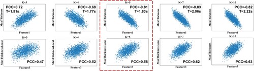
At the same time, the value of neighborhood parameter $K$ of K-domain was crucial for capturing geometric features. Setting $K$ too large or too small may affect the capture of the manifold structure within the dataset and can also affect computational efficiency. Figure 5 shows the feature extraction performance for $K=3,4,5,6,7,10$. The feature extraction time (T) is tested on an Intel Core i7 CPU (2.90 GHz). Finally, the $K$ is set to 5. At this setting, the features captured by ISOMAP are clearly correlated with the maximum relative thickness and its position of the airfoil, and the time of feature learning is relatively short.

Figure 5. Variation of correlation and time with $\text{K}$ value.

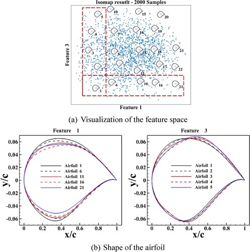
As shown in Figure 6(a), the corresponding airfoils are displayed in the 2D space composed of feature 1 and feature 3. Figure 6(b) provides a comparison of the profiles of the airfoils from the first row and the first column. The geometric parameters of the airfoil changed noticeably with variations in features.

Figure 6. Extracting features of the airfoil by using ISOMAP. (a) Visualization of the feature space; (b) Shape of the airfoil

3.2. Visual analysis of correlations

We assessed the aerodynamic performance of all airfoils in the database through CFD simulations to analyze their correlations with the geometric features. The distribution coefficient of surface pressure and the contours of pressure corresponding to Figure 6(b) are shown in Figure 7. $C_l$, $C_d$, and $C_m$ are the coefficients of lift, drag, and moment. Note that feature 1 was mainly linked to the height of the suction peak (Li et al., 2018; McLean, 2012), and influenced the intensity of the shockwave. Feature 3 was mainly linked to the fluctuations in pressure on the suction platform (Li et al., 2018; McLean, 2012), and influenced the form and position of the shockwaves. As the value of feature 3 increase, the airfoils exhibited double shockwaves. The results indicated a correlation between the geometric features captured by ISOMAP and the aerodynamic performance of the airfoils.

Figure 7. Visualization of geometric features and distributed forces. (a) Airfoils and the distribution of their pressure coefficients; (b) Contours of the pressure coefficient

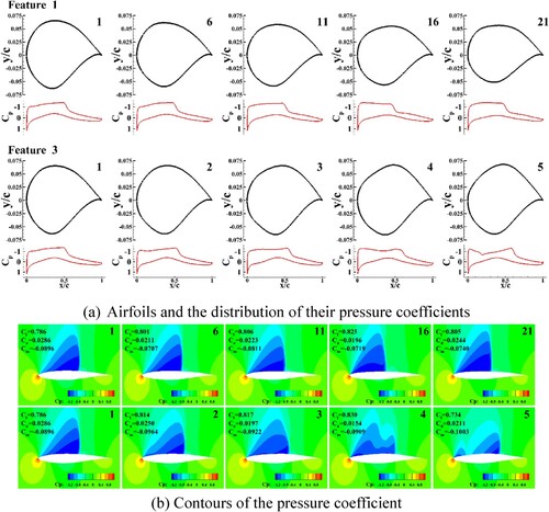
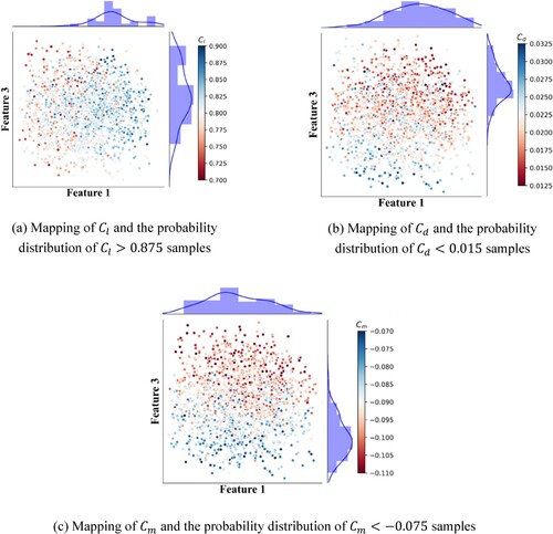
Figure 8 visualizes the distributions of $C_l$, $C_d$, and $C_m$ in feature space $\mathbf{\Psi }$. The aerodynamic coefficients correspond to the changes in color from red to blue. The magnitudes of the aerodynamic forces can be clearly differentiated in the feature space. $C_l$ was mainly correlated with feature 1. A larger feature 1 implied a higher probability that the corresponding airfoil had a larger $C_l$ (blue color). $C_d$ and $C_m$ were associated with feature 3. As feature 3 increased, both $C_d$ and $C_m$ decreased overall (from blue to red). These results demonstrate the correlation between the features and the integrated forces. The blue line and bar chart in Figure 8 are the probability distribution of samples satisfying the conditions $C_l>0.875$, $C_d<0.015$, and $C_m>-0.075$ in the feature space. Airfoils satisfying the thresholds of $C_l$, $C_d$, and $C_m$ were concentrated in the positive halves of features 1 and 3, and the negative half of feature 3, respectively. The geometric features of the airfoil located in these local regions implied that some of its aerodynamic coefficients are likely to satisfy the conditions.

Figure 8. Visualization of integrated forces in the feature space. (a) Mapping of ${\text{C}}_{\text{l}}$ and the probability distribution of ${\text{C}}_{\text{l}}>0.875$ samples; (b) Mapping of ${\text{C}}_{\text{d}}$ and the probability distribution of ${\text{C}}_{\text{d}}<0.015$ samples; (c) Mapping of ${\text{C}}_{\text{m}}$ and the probability distribution of ${\text{C}}_{\text{m}}<-0.075$ samples

4. Aerodynamic shape optimization based on geometric feature filtering

The analysis in section 3 makes it clear that the selected geometric features are correlated with aerodynamic performance. Airfoils with good aerodynamic performance tend to located in a local region of the geometric feature space. For example, if an airfoil is located in the positive half of feature 3 in the feature space of Figure 8, there is a high probability of the coefficient of drag being low. Therefore, the aerodynamic performance of the airfoil can be preliminarily assessed by its geometric features. Based on this, we proposed an efficient method for ASO in this section.

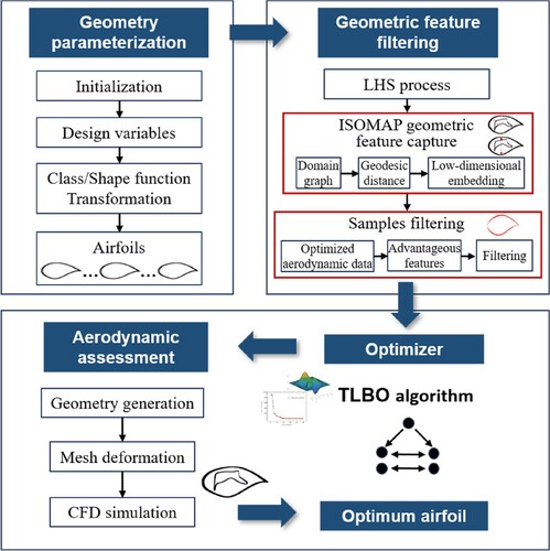
Figure 9 shows that the proposed method involves geometric parametrization, the filtering of geometric features, an optimizer, and the evaluation of aerodynamic performance. The CST method parametrizes the shape of the airfoils. Unsupervised ISOMAP captures the geometric features of airfoil database generated through LHS. Then, a filtering criterion based on the geometric features is established to filter out the shapes with a high probability of poor aerodynamic performance during the optimization process. Each candidate airfoil, as searched by the optimizer, is projected into the geometric feature space to assess its aerodynamic performance. The airfoil should satisfy the filtering criteria before being subjected to mesh deformation based on radial basis function-based interpolation (Jakobsson & Amoignon, 2007) and CFD simulations. The Teaching – Learning-based Optimization (TLBO) algorithm (Rao et al., 2011; Rao & Patel, 2012) is used as the optimizer owing to its parameter-free nature and strong capabilities of optimization. The TLBO algorithm is provided in Appendix A.

Figure 9. Overall framework for the optimization of the aerodynamic shape of the airfoils by using geometric feature filtering.

The detailed process of optimization is shown in Figure 10. ISOMAP takes the matrix $\mathit{X}=\left\{{\mathit{x}}_{\mathit{i}}ϵR^n|i=1,2,\dots ,N\right\}$ as input, where ${\mathit{x}}_{\mathit{i}}$ represents the $n$-dimensional coordinates of the airfoil and $i$ is the number of airfoils. The geometric features $\mathit{V}=\left\{{\mathit{v}}_{\mathit{i}}ϵR^m|i=1,2,\dots ,N\right\}$ is then obtained as follows: (8) $V=F\left(\mathit{X}\right)$(8) where $F\left(\mathit{X}\right)$ represents the operator of ISOMAP.

Figure 10. Detailed process of optimization of the aerodynamic shape of the airfoil.

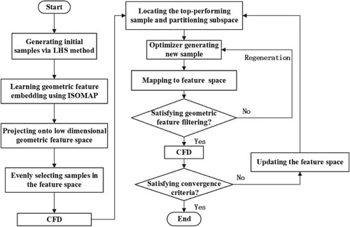
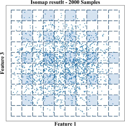
The geometric features correlated with aerodynamic performance are selected to construct a low-dimensional feature space $\mathbf{\Psi }$. Samples are uniformly sampled from $\mathbf{\Psi }$ for the CFD simulations to identify the location of the subspace ${\mathbf{\Psi }}^{\mathbf{\prime }}$ with good aerodynamic performance, and serve as initial samples for the optimizer. Sampling affects the accuracy of feature subspace localization and sample filtering. Therefore, a sampling method is proposed to cover the majority of the feature space evenly while minimizing computational costs. This method divides the boundaries based on the maximum and minimum values of the features. The boundaries are uniformly divided. The sampling regions are selected at intervals. A sample is randomly chosen within the selected regions as the initial airfoil design. As shown in Figure 11, the blue shadows are the selected sampling regions.

Figure 11. Uniform initial sampling method for feature space

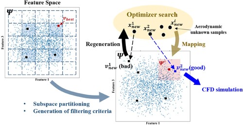
After obtaining samples in the sampling regions, the process of screening samples using geometric features is shown Figure 12. Centered on the feature ${\mathit{v}}_{\mathit{best}}$ of the optimal aerodynamic sample, a subspace ${\mathbf{\Psi }}^{\mathbf{\prime }}$ (pink shadow) is defined as the filter criterion. The range of ${\mathbf{\Psi }}^{\mathbf{\prime }}$ is proportionally scaled down from the boundary of $\mathbf{\Psi }$ with a scaling factor λ. Then, each new sample ${\mathit{x}}_{\mathit{new}}^{\mathit{i}}$ searched by the optimizer is brought into Eq. (8)(A1) ${\mathit{X}}^{\mathit{mean}}=\frac{{\sum }_i^{N_p}{\mathit{X}}^{\mathit{S}}}{N_p},$(A1) to obtain geometric feature ${\mathit{v}}_{\mathit{new}}^{\mathit{i}}$, where $i$ represents the index of the sample. If ${\mathit{v}}_{\mathit{new}}^{\mathit{i}}\in {\mathbf{\Psi }}^{\mathbf{\prime }}$, this means that ${\mathit{x}}_{\mathit{new}}^{\mathit{i}}$ probably delivers good aerodynamic performance, so ${\mathit{x}}_{\mathit{new}}^{\mathit{i}}$ will be retained and subjected to CFD simulation; otherwise, the optimizer regenerates a new sample ${\mathit{x}}_{\mathit{new}}^{{\mathit{i}}^{\mathbf{\prime }}}$ until its position ${\mathit{v}}_{\mathit{new}}^{{\mathit{i}}^{\mathbf{\prime }}}\in {\mathbf{\Psi }}^{\mathbf{\prime }}$. To maintain the continuity and directionality of the evolutionary optimization, the regenerated samples follow the mechanism of variation of the optimizer rather than being randomly generated. If the condition cannot be met after several attempts at regeneration, the optimizer automatically proceeds to the next step.

Figure 12. The process of screening samples using geometric features

The final step involves conducting CFD simulations on the filtered samples. As the optimizer searches iteratively, all generated historical aerodynamic data are continuously added back to the airfoil database, and are used to update $\mathbf{\Psi }$, ${\mathbf{\Psi }}^{\mathbf{\prime }}$, and ${\mathit{v}}_{\mathit{best}}$ until the algorithm converges.

5. Aerodynamic shape optimization of RAE2822 airfoil

In this section, we apply the proposed method to the unconstrained and constrained optimizations of the aerodynamic shape of the RAE2822 airfoil in transonic viscous flow to validate its effectiveness.

5.1. Example 1: Unconstrained optimization of airfoil

The problem of the unconstrained ASO of the RAE2822 airfoil can be mathematically expressed as follows: $\mathrm{Max}{C}_l/C_d$

The design space and initial geometric feature space $\mathbf{\Psi }$ were consistent with those described in Sec. 3. The proposed method (TLBO-ISOMAP) and the traditional TLBO method without geometric feature filtering were used for optimization, and their performance was compared. The random seeds (Madhyastha & Jain, 2019) of all methods were the same to ensure the generation of the same pseudo-random number sequence. The parameters of the TLBO algorithm were consistent in the two methods. The population size ($N_P$) was set to 10 and the maximum number of generations was set to 50. In each generation, a total of 2$N_P$ CFD simulations were conducted in both the ‘teaching phase’ and the ‘learning phase.’ The detailed principles of the algorithm are provided in Appendix A. A total of 23 airfoils were uniformly selected in $\mathbf{\Psi }$ to preliminarily determine the feature subspace ${\mathbf{\Psi }}^{\mathbf{\prime }}$. Meanwhile, the best $N_P$ airfoils in terms of aerodynamic performance were chosen as the initial population for TLBO-ISOMAP and TLBO to ensure a fair comparison.

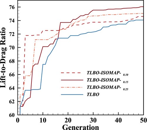
The history of convergence of the optimization is shown in Figure 13. We provide the results of the TLBO-ISOMAP method with scaling factors $\lambda =0.10,0.15,\text{and}0.25$ for the feature subspace. Although the optimization results in all cases are better than the TLBO method, different values of the scaling factor can also affect the improvement of optimization efficiency. A scaling value that is too small may lead to the optimization results falling into local optima; A scaling value that is too large may reduce the effectiveness of the filtering criteria, as it could cover more poor-performance sample features in the feature subspace. The lift-to-drag ratio of the airfoil optimized by the TLBO method increased from 42.2–74.1, an improvement of 75.6%. The airfoil optimized by the TLBO-ISOMAP-${\lambda }_{0.15}$ method increased the lift-to-drag ratio from 42.2–76.0, an improvement of 80.1%. The TLBO-ISOMAP-${\lambda }_{0.15}$ method obtained the final optimization of the TLBO method in about 20 generations, and improved the efficiency of optimization by approximately 60%.

Figure 13. Convergence histories

The optimized airfoil and its pressure distribution are shown in Figure 14. It shifted the shockwaves toward the leading edge to significantly weaken their intensity.

Figure 14. Comparison of the results of unconstrained optimization. (a) Comparison of optimized and initial airfoils; (b) Comparison of the distributions of wall pressure between the optimized and initial airfoils

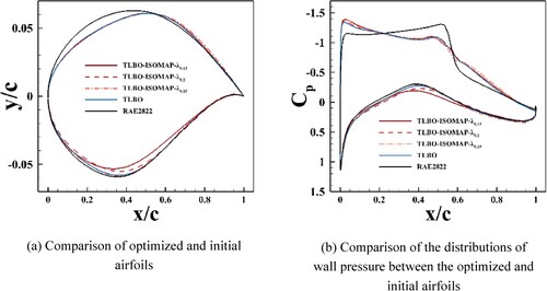
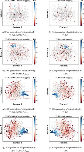
Figure 15 shows the mapping of the geometric features of airfoils generated by the TLBO-ISOMAP-${\lambda }_{0.15}$ and TLBO methods in the first, 10th, 30th, and 50th generations. The feature space was continuously updated. The red dashed box is the feature subspace of the filtered samples, while the gray points are the feature mappings of the initial database. The colored markers represent the optimized samples, with the range of colors from red to blue corresponding to changes in the lift-to-drag ratio (L/D). The pentagrams denote the locations of the maximum L/D. Overall, the samples generated by the TLBO-ISOMAP-${\lambda }_{0.15}$ method exhibite better aerodynamic performance than those generated by the TLBO method. Airfoils with higher L/D (blue points) exhibite a clear clustering. The proposed method can quickly locate these advantageous regions and generate filtering criteria to improve sample quality, which may be one of the reasons for improving optimization efficiency.

Figure 15. Results of optimized feature projection by TLBO-ISOMAP-${\lambda }_{0.15}$ and TLBO. (a) First generation of optimization by TLBO-ISOMAP-${\lambda }_{0.15};$(b) First generation of optimization by TLBO; (c) 10th generation of optimization by TLBO-ISOMAP-${\lambda }_{0.15}$; (d) 10th generation of optimization by TLBO; (e) 30th generation of optimization by TLBO-ISOMAP-${\lambda }_{0.15}$; (f) 30th generation of optimization by TLBO; (g) $5$0th generation of optimization by TLBO-ISOMAP-${\lambda }_{0.15}$; (h) 50th generation of optimization by TLBO

5.2. Example 2: Constrained optimization of airfoil

Three cases of the constrained ASO were used to compare optimization performance. The statement of optimization problem is shown in Table II.

Table 2. Optimization problem statement

	Case 1		Case 2		Case 3
	Function	Description	Function	Description	Function	Description
$\mathrm{Min}$	$C_d$	Drag coefficient	$C_d$	Drag coefficient	$C_d$	Drag coefficient
$S.t.$	$C_l\ge 0.824$	Lift constraint	$C_l\ge 0.824$	Lift constraint	$C_l\ge 0.824$	Lift constraint
	$C_m\ge -0.092$	Pitching moment constraint	$C_m\ge -0.092$	Pitching moment constraint	$C_m\ge -0.092$	Pitching moment constraint
	$A\ge A_{\mathrm{initial}}$	Area constraint	$t_{\max }\ge 12\mathrm{\%}$	Maximum relative thickness constraint	$t_{\max }=12\mathrm{\%}$	Maximum relative thickness constraint
					$l_{t_{\max }}=0.38$	Maximum relative thickness position constraint

The penalty function is used to transform the problem of constrained optimization into that of unconstrained optimization as follows: $\mathrm{Min}{C}_d^p=C_d+\mu \cdot \left(\sum _{i=1}^{m}max\left(0,g_i\right)+\sum _{j=1}^n|h_j|\right)$

where $\mu$ is the penalty factor. $g_i$ and $h_j$ are inequality and equality constraints.

$\mu$ was set to 10. The feature space, parameter settings, and initial samples were consistent with those given in Sec.5.1. After some tests, the performance was better with the scaling factor $\lambda$ set to 0.2. We compared the results of optimization of the TLBO-ISOMAP-${\lambda }_{0.2}$, TLBO and Bayesian Adaptive Direct Search (BADS) (Singh & Acerbi, 2023) methods. The TLBO-ISOMAP-${\lambda }_{0.2}$ method divided the feature subspace based on the optimal solution of the penalty function. The BADS is a fast and robust black-box optimization algorithm. It finds the optimal solution through local Bayesian optimization and searching in the neighborhood space.

The convergence histories are shown in Figure 16. The optimization results for the three cases are compared in Table III. The number of CFD simulations for all methods corresponds to the iterations required to achieve the optimal value of the TLBO method. It can be seen that the proposed method achieved the best results for various optimization problems, indicating its good engineering application value. The proposed method obtained the final solution of TLBO method with a reduction in the number of CFD simulations by 45.2% to 62.5% compared to the TLBO method. Although the state-of-the-art BADS method had the potential to quickly find its optimal value, the final converged results were inferior to those of the proposed method in all cases. The optimized airfoils and its pressure distribution are shown in Figure 17. The pressure distribution of optimized airfoils was smoother than the original airfoil, which is the main reason for the weaker shockwaves.

Table 3. Result of different constrained optimization

Case	Method	$C_d^p$	CFD iterations required to achieve TLBO optimal value	Increment
Original	…	0.0195		…
Case 1	TLBO-ISOMAP-${\lambda }_{0.2}$	0.0116	460	40.5%
	TLBO	0.0120	840	38.5%
	BADS	0.0119	192	39.0%
Case 2	TLBO-ISOMAP-${\lambda }_{0.2}$	0.0115	520	41.0%
	TLBO	0.0119	980	39.0%
	BADS	0.0126	Not reached	38.5%
Case 3	TLBO-ISOMAP-${\lambda }_{0.2}$	0.0160	360	17.9%
	TLBO	0.0172	960	11.8%
	BADS	0.0169	298	13.3%

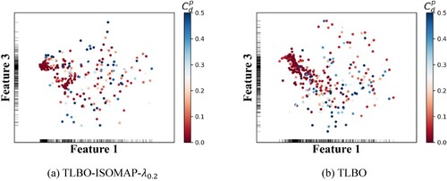
The geometric features of the top 40% of samples in terms of aerodynamic performance, optimized by the TLBO-ISOMAP-${\lambda }_{0.2}$ and TLBO methods in case 1, are shown in Figure 18. The range of colors from red to blue corresponds to changes in the value of $C_d^p$. It is evident that the aerodynamic performance of samples generated by the proposed method was generally better than those generated by the TLBO method. Figure 19 and Figure 20 respectively depict the distribution density in the feature space and the corresponding $C_d^p$ values of the samples generated by the two methods from the 30th to the 50th generations. It can be observed that samples with lower $C_d^p$ values are more densely distributed in high-density regions. This phenomenon is more pronounced with the proposed method, indicating an overall improvement in sample quality.

Figure 16. Convergence histories. (a) Case 1; (b) Case 2; (c) Case 3

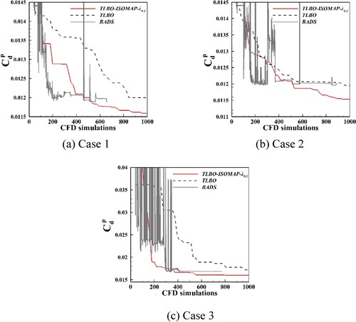
Figure 17. Pressure distributions and airfoils of different constrained optimization. (a) Case 1; (b) Case 2; (c) Case 3

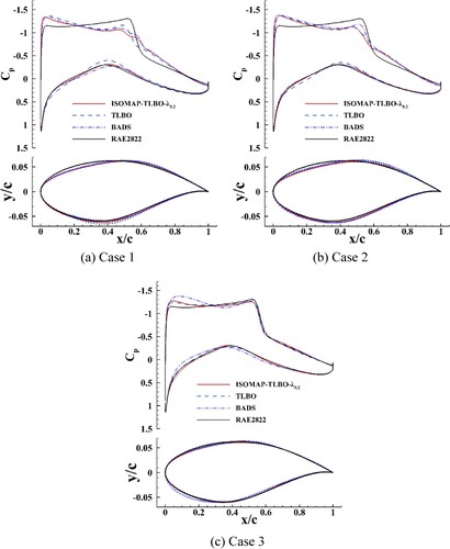
Figure 18. Projections of the top 40% of the samples in terms of aerodynamic performance in case 1. (a) Projection of the sample generated by TLBO-ISOMAP-${\lambda }_{0.2}$; (b) Projection of the sample generated by TLBO

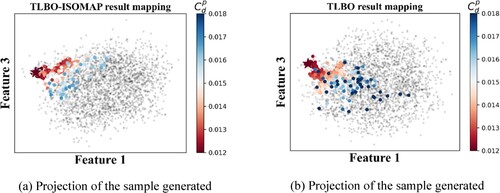
Figure 19. Distribution density of samples generated in generations 30–50 for case 1. (a) TLBO-ISOMAP-${\lambda }_{0.2}$; (b) TLBO

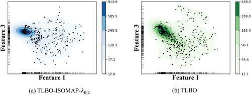
Figure 20. Projection of ${\text{C}}_{\text{d}}^{\text{p}}$ of samples generated in generations 30–50 for case 1. (a) TLBO-ISOMAP-${\lambda }_{0.2}$; (b) TLBO

The localized feature space of samples generated by the proposed method is shown in Figure 21. Figure 21(a) displays the shapes and pressure distributions of the airfoils from local samples. Figure 21(b) provides a comparison of their shapes in this localized feature area. Approximately 78.3% of the samples are marked in red ($C_d^p<0.0120$) in this region, reflecting a high probability of obtaining airfoils with relatively small values of $C_d^p$. These airfoils seem to have a certain degree of convergence because they exhibit similar shapes and geometric features. It may indicate that airfoils with good aerodynamic performance have some common geometric features. Although there is a small probability of including poor aerodynamic performance, if these geometric features can be quickly identified at the beginning of optimization, it may help reduce the blind search in optimization.

Figure 21. Visualization of the local feature space of samples generated by TLBO-ISOMAP-${\lambda }_{0.2}$ in generations 30–50 for case 1. (a) Visualization of airfoils and their pressure distributions; (b) Comparison of airfoils

6. Conclusion

To mitigate the blind search in iterative methods of ASO, which inevitably leads to shapes with poor aerodynamic performance, this study captured the correlation between geometric features of airfoils and their aerodynamic performance, and proposed an efficient method to improve optimization efficiency by using this knowledge. Unsupervised ISOMAP captured geometric features correlated with aerodynamic performance at low cost in the absence of aerodynamic information. This correlation knowledge was used to preliminarily evaluate the aerodynamic performance of airfoils. Shapes with a high probability of poor aerodynamic performance were filtered out during the optimization process before conducting CFD simulations, which effectively improved sample quality. The proposed method was used to learn the geometric features of deformed shapes based on the RAE2822 airfoil. Constrained and unconstrained transonic ASO of the RAE2822 airfoil were conducted to analyze and verify the effectiveness of the proposed method. The following conclusions can be drawn:

1. ISOMAP successfully captured geometric features correlated with aerodynamic performance in an unsupervised manner by assessing the correlation between these features and airfoil parameters that influence aerodynamic performance. When using ISOMAP, attention should be paid to the hyperparameter settings for constructing the neighborhood graph because they may affect the effectiveness of feature extraction or computational efficiency.

2. The proposed method achieved satisfactory results for various optimization problems, demonstrating its significant engineering practical value. It can improve the efficiency of optimization by over 50% compared with the conventional TLBO method. The scaling factor $\lambda$ of the feature subspace may impact the optimization effectiveness because a large $\lambda$ may compromise optimization performance, while a small $\lambda$ may lead to local optima.

3. Visual analysis indicated that samples with good aerodynamic performance generated during the optimization process showed a noticeable clustering phenomenon in the selected feature space. The proposed method results in higher density distribution in the clustered regions, indicating an improvement in sample quality during the optimization process.

The knowledge of geometric features correlated with aerodynamic performance has the potential to be embedded into other optimization frameworks to further enhance the efficiency of ASO. For example, it could assist in improving the quality of samples in surrogate-based optimization frameworks. Future work could further explore other geometric features that can more significantly differentiate aerodynamic performance.

Disclosure statement

No potential conflict of interest was reported by the author(s).

Data availability

Data will be made available on request.

Additional information

Funding

This work was supported by the National Natural Science Foundation of China Youth Fund (Grant number 11902235), the National Key Research and Development Program of China (Grant number 2022YFB4300200), the National Key Research and Development Program of China (Grant number 2023YFB4203400), and the Basic Research Program of Taicang (Grant number TC2023JC10).

Appendix A:

Teaching-learning-based optimization algorithm

The TLBO is a kind of gradient-free algorithm based on the pattern of ‘teaching’ and ‘learning’. It does not involve tuning hyperparameters that affect the optimization results, except for setting the population size ($N_P$). The ‘knowledge level’ of students and teacher is improved in teacher phase and learner phase. Detailed steps are introduced as follows:

Step1: Set parameters: define the $N_P$; set termination conditions, such as the maximum number of iteration steps $G_{\max }$.

Step2: Initialize the class (population) and evaluate the individuals’ knowledge level (fitness value).

Step3: Select the best individual as the teacher ${\mathit{X}}^{\mathit{T}}$, and other individuals are called students ${\mathit{X}}^{\mathit{S}}$. Calculate the mean of students ${\mathit{X}}^{\mathit{mean}}$.

The formula for ${\mathit{X}}^{\mathit{mean}}$ is as follows: (A1) ${\mathit{X}}^{\mathit{mean}}=\frac{{\sum }_i^{N_p}{\mathit{X}}^{\mathit{S}}}{N_p},$(A1)

Step 4: Teacher phase: ${\mathit{X}}^{\mathit{S}}$ is updated according to the difference between ${\mathit{X}}^{\mathit{T}}$ and${\mathit{X}}^{\mathit{mean}}$: (A2) ${\mathit{X}}_{\mathit{i}}^{\text{new}}={\mathit{X}}_{\mathit{i}}^{\mathit{old}}+r_i\left({\mathit{X}}^{\mathit{T}}-T_F{\mathit{X}}^{\mathit{mean}}\right),$(A2) (A3) $\{\begin{array}{c}{\mathit{X}}_{\mathit{i}}^{\mathit{S}}={\mathit{X}}_{\mathit{i}}^{\mathit{new}},\mathrm{iff}\left({\mathit{X}}_{\mathit{i}}^{\mathit{new}}\right)\le f\left({\mathit{X}}_{\mathit{i}}^{\mathit{old}}\right)\\ {\mathit{X}}_{\mathit{i}}^{\mathit{S}}={\mathit{X}}_{\mathit{i}}^{\mathit{old}},\mathrm{iff}\left({\mathit{X}}_{\mathit{i}}^{\mathit{new}}\right)>f\left({\mathit{X}}_{\mathit{i}}^{\mathit{old}}\right)\end{array},$(A3) where ${\text{r}}_i$ is a random factor that generates a 1-by-1 matrix with uniformly distributed random numbers between 0 and 1. $T_F$ is the teaching factor, randomly generating a floating-point number between 1 and 2, and rounding it to the nearest integer.

Step 5: Learner phase: Randomly select two students ${\mathit{X}}_{\mathit{i}}^{\mathit{S}}$ and ${\mathit{X}}_{\mathit{j}}^{\mathit{S}}$, allowing them to learn from each other. They can update themselves using the following formula: (A6) $\{\begin{array}{c}{\mathit{X}}_{\mathit{i}}^{\mathit{S},\mathit{G}+1}={\mathit{X}}_{\mathit{i}}^{\mathit{S},\mathit{G}}+r_i\left({\mathit{X}}_{\mathit{i}}^{\mathit{S},\mathit{G}}-{\mathit{X}}_{\mathit{j}}^{\mathit{S},\mathit{G}}\right),\text{ if }f\left({\mathit{X}}_{\mathit{i}}^{\mathit{S},\mathit{G}}\right)<f\left({\mathit{X}}_{\mathit{j}}^{\mathit{S},\mathit{G}}\right)\\ {\mathit{X}}_{\mathit{i}}^{\mathit{S},\mathit{G}+1}={\mathit{X}}_{\mathit{i}}^{\mathit{S},\mathit{G}}+r_i\left({\mathit{X}}_{\mathit{j}}^{\mathit{S},\mathit{G}}-{\mathit{X}}_{\mathit{i}}^{\mathit{S},\mathit{G}}\right),\text{ if }f\left({\mathit{X}}_{\mathit{i}}^{\mathit{S},\mathit{G}}\right)\ge f\left({\mathit{X}}_{\mathit{j}}^{\mathit{S},\mathit{G}}\right)\end{array},$(A6)

Step 6: Determine whether the convergence condition is satisfied. If it is satisfied, the optimization process ends; otherwise, return to Step 3, and continue the process.

References

- Achour, G., Sung, W. J., Pinon-Fischer, O. J., & Mavris, D. N. (2020). Development of a conditional generative adversarial network for airfoil shape optimization. AIAA Scitech 2020 Forum. https://doi.org/10.2514/6.2020-2261
- Adjei, R. A., & Fan, C. (2024). Multi-objective design optimization of a transonic axial fan stage using sparse active subspaces. Engineering Applications of Computational Fluid Mechanics, 18(1), 2325488. https://doi.org/10.1080/19942060.2024.2325488
- Bhola, S., Pawar, S., Balaprakash, P., & Maulik, R. (2023). Multi-fidelity reinforcement learning framework for shape optimization. Journal of Computational Physics, 482, 112018. https://doi.org/10.1016/j.jcp.2023.112018
- Bletsos, G., Kühl, N., & Rung, T. (2021). Adjoint-based shape optimization for the minimization of flow-induced hemolysis in biomedical applications. Engineering Applications of Computational Fluid Mechanics, 15(1), 1095–1112. https://doi.org/10.1080/19942060.2021.1943532
- Buja, A., Swayne, D. F., Littman, M. L., Dean, N., Hofmann, H., & Chen, L. (2008). Data visualization With multidimensional scaling. Journal of Computational and Graphical Statistics, 17(2), 444–472. https://doi.org/10.1198/106186008X318440
- Chen, W., Chiu, K., & Fuge, M. (2019). Aerodynamic design optimization and shape exploration using generative adversarial networks. AIAA Scitech 2019 Forum, https://doi.org/10.2514/6.2019-2351
- Chen, W., Fuge, M., & Chazan, J. (2017). Design manifolds capture the intrinsic complexity and dimension of design spaces. Journal of Mechanical Design, 139(5), 051102. https://doi.org/10.1115/1.4036134
- Dai Z., Li T., Xiang Z. R., Zhang W., & Zhang J. (2023). Aerodynamic multi-objective optimization on train nose shape using feedforward neural network and sample expansion strategy. Engineering Applications of Computational Fluid Mechanics, 17(1), 2226187. https://doi.org/10.1080/19942060.2023.2226187
- Dai, J., Liu, P., Qu, Q., Li, L., & Niu, T. (2022). Aerodynamic optimization of high-lift devices using a 2D-to-3D optimization method based on deep reinforcement learning and transfer learning. Aerospace Science and Technology, 121, 107348. https://doi.org/10.1016/j.ast.2022.107348
- Decker, K., Schwartz, H. D., & Mavris, D. (2020). Dimensionality reduction techniques applied to the design of hypersonic aerial systems. Aiaa Aviation 2020 Forum, https://doi.org/10.2514/6.2020-3003
- Dijkstra, E. W. (1959). A note on two problems in connexion with graphs. Numerische Mathematik, 1(1), 269–271. https://doi.org/10.1007/BF01386390
- Du, X., He, P., & Martins, J. R. R. A. (2021). Rapid airfoil design optimization via neural networks-based parameterization and surrogate modeling. Aerospace Science and Technology, 113, 106701. https://doi.org/10.1016/j.ast.2021.106701
- Esfahanian, V., Izadi, M. J., Bashi, H., Ansari, M., Tavakoli, A., & Kordi, M. (2024). Aerodynamic shape optimization of gas turbines: A deep learning surrogate model approach. Structural and Multidisciplinary Optimization, 67(1), 2. https://doi.org/10.1007/s00158-023-03703-9
- Floyd, R. W. (1962). Algorithm 97: Shortest path. Communications of the ACM, 5(6), 345–345. https://doi.org/10.1145/367766.368168
- Fukami, K., & Taira, K. (2023). Grasping extreme aerodynamics on a low-dimensional manifold. Nature Communications, 14(1), 6480. https://doi.org/10.1038/s41467-023-42213-6
- Izenman, A. J. (2012). Introduction to manifold learning. WIRES Computational Statistics, 4(5), 439–446. https://doi.org/10.1002/wics.1222
- Jakobsson, S., & Amoignon, O. (2007). Mesh deformation using radial basis functions for gradient-based aerodynamic shape optimization. Computers & Fluids, 36(6), 1119–1136. https://doi.org/10.1016/j.compfluid.2006.11.002
- Jiang H., Xu M., & Yao W. (2022). Aerodynamic shape optimization Of co-Flow jet airfoil using a multi-Island genetic algorithm. Physics of Fluids, 34(12), 125120. https://doi.org/10.1063/5.0124372
- Kaya H., & Tuncer İ. H. (2021). Discrete adjoint-based aerodynamic shape optimization framework for natural laminar flows. AIAA Journal 30, 1–16. https://doi.org/10.2514/1.J059923.
- Kou, J., Botero-Bolívar, L., Ballano, R., Marino, O., De Santana, L., Valero, E., & Ferrer, E. (2023). Aeroacoustic airfoil shape optimization enhanced by autoencoders. Expert Systems with Applications, 217, 119513. https://doi.org/10.1016/j.eswa.2023.119513
- Kulfan, B. (2007). A universal parametric geometry representation method - "CST". 45th AIAA Aerospace Sciences Meeting and Exhibit, https://doi.org/10.2514/6.2007-62
- Li, J., Cai, J., & Qu, K. (2019a). Surrogate-based aerodynamic shape optimization with the active subspace method. Structural and Multidisciplinary Optimization, 59(2), 403–419. https://doi.org/10.1007/s00158-018-2073-5
- Li, R., Deng, K., Zhang, Y., & Chen, H. (2018). Pressure distribution guided supercritical wing optimization. Chinese Journal of Aeronautics, 31(9), 1842–1854. https://doi.org/10.1016/j.cja.2018.06.021
- Li, J., He, S., & Martins, J. R. R. A. (2019b). Data-driven constraint approach to ensure low-speed performance in transonic aerodynamic shape optimization. Aerospace Science and Technology, 92, 536–550. https://doi.org/10.1016/j.ast.2019.06.008
- Madhyastha, P., & Jain, R. (2019). On model stability as a function of random seed. arxiv preprint arxiv:1909.10447. http://arxiv.org/abs/1909.10447.
- Marsland, S. (2015). Machine learning: An algorithmic perspective (2nd ed.). CRC Press.
- Martins, J. R. R. A. (2022). Aerodynamic design optimization: Challenges and perspectives. Computers & Fluids, 239, 105391. https://doi.org/10.1016/j.compfluid.2022.105391
- Mckay, M. D., Beckman, R. J., & Conover, W. J. (2000). A comparison of three methods for selecting values of input variables in the analysis of output from a computer code. Technometrics, 42(1), 55–61. https://doi.org/10.1080/00401706.2000.10485979
- McLean D. (2012). Understanding aerodynamics: Arguing from the real physics. 1st ed. Wiley. https://doi.org/10.1002/9781118454190
- Mohebbi F., Evans B., & Sellier M. (2021). On an exact step length in gradient-based aerodynamic shape optimization—part II: Viscous flows. Fluids, 6(3), 106. https://doi.org/10.3390/fluids6030106
- Noyel, G., Angulo, J., & Jeulin, D. (2011). Fast computation of all pairs of geodesic distances. Image Analysis & Stereology, 30(2), 101. https://doi.org/10.5566/ias.v30.p101-109
- Oliveira N.L., Rendón M.A., Lemonge A.C.D.C., & Hallak P.H. (2024). Multi-objective optimum design of propellers using the blade element theory and evolutionary algorithms. Evolutionary Intelligence, 17(3), 1623-1653. https://doi.org/10.1007/s12065-023-00855-x
- Prautzsch H., Boehm W., & Paluszny M. (2002). Bézier and B-spline techniques. Springer Berlin Heidelberg. https://doi.org/10.1007/978-3-662-04919-8
- Qian J., Cheng Y., Zhang J., Liu J., & Zhan D. (2021). A parallel constrained efficient global optimization algorithm for expensive constrained optimization problems. Engineering Optimization, 53(2), 300-320. https://doi.org/10.1080/0305215X.2020.1722118
- Rao, R. V., & Patel, V. (2012). An improved teaching-learning-based optimization algorithm for solving unconstrained optimization problems. Scientia Iranica, 20(3), 710–720. https://doi.org/10.1016/j.scient.2012.12.005
- Rao, R. V., Savsani, V. J., & Vakharia, D. P. (2011). Teaching–learning-based optimization: A novel method for constrained mechanical design optimization problems. Computer-Aided Design, 43(3), 303–315. https://doi.org/10.1016/j.cad.2010.12.015
- Raul, V., & Leifsson, L. (2021). Surrogate-based aerodynamic shape optimization for delaying airfoil dynamic stall using kriging regression and infill criteria. Aerospace Science and Technology, 111, 106555. https://doi.org/10.1016/j.ast.2021.10655
- Samareh, J. (2004). Aerodynamic shape optimization based on free-form deformation. 10th AIAA/ISSMO Multidisciplinary Analysis and Optimization Conference, https://doi.org/10.2514/6.2004-4630
- Shirvani, A., Nili-Ahmadabadi, M., & Ha, M. Y. (2023). Machine learning-accelerated aerodynamic inverse design. Engineering Applications of Computational Fluid Mechanics, 17(1), 2237611. https://doi.org/10.1080/19942060.2023.2237611
- Singh G. S., & Acerbi L. (2023). PyBADS: Fast and robust black-box optimization in Python. arxiv preprint arxiv:2306.15576. http://arxiv.org/abs/2306.15576 .
- Tenenbaum, J. B., Silva, V. D., & Langford, J. C. (2000). A global geometric framework for nonlinear dimensionality reduction. Science, 290(5500), 2319–2323. https://doi.org/10.1126/science.290.5500.2319
- Wang, K., Han, Z. H., Zhang, K. S., & Song, W. P. (2023b). An efficient geometric constraint handling method for surrogate-based aerodynamic shape optimization. Engineering Applications of Computational Fluid Mechanics, 24(1), 2153173. https://doi.org/10.1080/19942060.2022.2153173
- Wang, C., Wang, L., Cao, C., Sun, G., Huang, Y., & Zhou, S. (2023a). Aerodynamic optimization framework for a three-dimensional nacelle based on deep manifold learning-assisted geometric multiple dimensionality reduction. Aerospace, 10(7), 573. https://doi.org/10.3390/aerospace10070573
- Wu N., Mader C. A., & Martins J. R. R. A. (2022). A gradient-Based sequential multifidelity approach to multidisciplinary design optimization. Structural and Multidisciplinary Optimization, 65(4), 131. https://doi.org/10.1007/s00158-022-03204-1
- Wu M. Y., Yuan X. Y., Chen Z. H., Wu W. T., Hua Y., & Aubry N. (2023). Airfoil shape optimization using genetic algorithm coupled deep neural networks. Physics of Fluids, 35(8), 085140. doi:10.1063/5.0160954
- Wu, X., Zhang, W., Peng, X., & Wang, Z. (2019). Benchmark aerodynamic shape optimization with the POD-based CST airfoil parametric method. Aerospace Science and Technology, 84, 632–640. https://doi.org/10.1016/j.ast.2018.08.005
- Yang Y., Xue Y., Zhao W., Yang H., & Wu C. (2024). Aerodynamic shape optimization based on proper orthogonal decomposition reparameterization under small training sets. Aerospace Science and Technology (Elmsford, N Y ), 147, 109072.
- Yang Y., Zhao W., Xue Y., Yang H., & Wu C. (2023). Improved automatic kernel construction for Gaussian process regression in small sample learning for predicting lift body aerodynamic performance. Physics of Fluids, 35(6). doi: 10.1063/5.0153970
- Yonekura, K., & Suzuki, K. (2021). Data-driven design exploration method using conditional variational autoencoder for airfoil design. Structural and Multidisciplinary Optimization, 64(2), 613–624. https://doi.org/10.1007/s00158-021-02851-0
- Zachary, J. G. (2017). Active subspaces of airfoil shape parameterizations. AIAA Journal, 56(5), 2003–2017. https://doi.org/10.2514/1.j056054.
- Zachary J. G. & Paul G. C. (2018). Active subspaces of airfoil shape parameterizations. AIAA Journal, 56(5), 2003–2017. https://doi.org/10.2514/1.j056054
- Zhang, W., Li, X., Ye, Z., & Jiang, Y. (2015). Mechanism of frequency lock-in in vortex-induced vibrations at low reynolds numbers. Journal of Fluid Mechanics, 783, 72–102. https://doi.org/10.1017/jfm.2015.548
- Zhang, W., Peng, X., Kou, J., & Wang, X. (2024). Heterogeneous data-driven aerodynamic modeling based on physical feature embedding. Chinese Journal of Aeronautics, 37(3), 1–6. https://doi.org/10.1016/j.cja.2023.11.010
- Zhang, X., Xie, F., Ji, T., Zhu, Z., & Zheng, Y. (2021). Multi-fidelity deep neural network surrogate model for aerodynamic shape optimization. Computer Methods in Applied Mechanics and Engineering, 373, 113485. https://doi.org/10.1016/j.cma.2020.113485