Computers in education: the association between computer use and test scores in primary school

ABSTRACT

This paper analyses the associations between computer use in schools and at home and test scores by using TIMSS data covering over 900,000 children in fourth grade. When controlling for school fixed effects, pupils who use computers at school, especially those who use them frequently are found to achieve less than students who never use computers. Daily computer use at home is negatively associated with test scores, although monthly, and sometimes weekly, use is positively associated with pupil performance. There is no significant difference between subjects and only small gender and country differences are observed. Moreover, the result suggests that the negative association of computer use at school is larger among low-performing pupils than for high-performing pupils. The findings suggest a negative association of computer use at school and test scores but do not reject the possibility that computers have a positive impact on test scores if computers are used optimally.

KEYWORDS:

• Computers
• economics of education
• productivity
• TIMSS

1. Introduction and background

Among policy makers, it is widely believed that investment in Information and Communications Technology (ICT) has an important role in improving education (Organisation for Economic Co-operation and Development [OECD], 2006, 2010). Supporters propose that tasks such as taking notes, information searches, and collaboration can be made more efficient than with more traditional methods such as pen and paper. Previous research on computers in education has, however, found mixed results and the estimated impacts are often small and insignificant. See, e.g., Bulman and Fairlie (2016) and Hall, Lundin, and Sibbmark (2019) for a literature overview.

An argument against computers in classrooms is that computers have a distraction effect. In a quasi-experiment, Carter, Greenberg, and Walker (2017) found that students at a military college who were allowed to use computers at lectures performed significantly worse than other students. Without supervision, students were more likely to use a computer for non-productive tasks, such as social media or chatting during lectures. Correspondingly, increased computer access did not improve grades or cognitive ability among younger children, and the computers were mostly used for entertainment purposes (Beuermann, Cristia, Cueto, Malamud, & Cruz-Aguayo, 2015).

Positive effects of computers are mostly found in studies where the intervention includes supervision and guided computer sessions. For example, Barrow, Markman, and Rouse (2009) report a positive effect of using computer-assisted learning in algebra classes among children. They suggest that the positive effect is explained by motivational factors. The computers let the pupils learn at their own pace, which makes the lectures more engaging. Similarly, Muralidharan, Singh, and Ganimian (2019) observed increased knowledge in Hindi and Maths among students who participated in after school programmes with computer access.¹

In contrast to the experimental approach, Fuchs and Wössmann (2004) examined the relationship of computer use and test scores with observational data from eighth graders in the Programme for International Student Assessment (PISA) study. They report an inverted u-shape between the frequency of computer use at school and test scores. Students who used computers a few times a year or several times a month achieved slightly higher maths scores than never users and significantly higher than students who used computers at school several times a week.

From experimental evidence, it seems like there is a distinction between increasing computer access or implementing computers in education with supervision. It is, therefore, interesting when Falck, Mang, and Wössmann (2018) focus on the effect of different computer activities in the classroom on test scores. They used data at teacher-level in each subject to exploit within-student between-subjects variation and found positive effects of using computers to look up information but adverse effects by using the computer to practice skills. The overall effect of computer use was, however, close to zero.

Studies such as Hull and Duch (2019) and Yanguas (2020) use quasi-experimental approaches as they exploit one-laptop-per-child programmes and evaluate the long-term effects of computers on a larger scale. Hull and Duch (2019) found the effects on test scores in mathematics to be small and the effects only appeared after a few years. In contrast, Yanguas (2020) did not find any positive effect of increased computer access on test scores or cognitive skills. In fact, the results suggest that educational attainment may even decrease by participating in the one-laptop-per-child programme.

This paper contributes to the current literature by studying the associations between computer use and test scores among young pupils. The analysis is based on data from 900,000 fourth graders from the 2011 and 2015 waves of the Trends in International Mathematics and Science Study (TIMSS).

The focus is on younger children, in contrast to the previous studies using TIMSS or PISA data, as there are reasons to believe that the association of computer use and test scores are different for 15-year-old students and 10-year-old children. For example, children who fall behind early in school tend to be disadvantaged later in their education (see, e.g., Hernandez, 2011). It is, therefore, of great interest to study computer use among children at younger ages.

Since the TIMSS study is based on observational data, this paper cannot provide a relationship with a causal interpretation such as an experimental study would. The computer use is not randomly distributed in the treatment and control group, which means that the findings in this study should be interpreted in terms of conditional correlations rather than as causal relationships.² On the other hand, the empirical approach allows for a larger set of observations than an experimental study. More importantly, the estimated results in observational studies are based on children’s actual computer use, instead of ideal or closely monitored computer use in an experimental setting. Both experimental and observational methods have their strengths and weaknesses. The experimental studies are beneficial in the sense that one can determine the actual treatment effect of computers in education. It is, however, debatable whether the result will reappear if computers are implemented under other circumstances than an experiment. A study with an observational approach can, therefore, complement experimental findings with larger external validity, even if estimated associations are not causal.

Previous studies using TIMSS or PISA data have either reported the result by each country separately or used country fixed effects to account for unobserved heterogeneity between countries. This paper contributes to the literature by instead using school fixed effects. This is important because there may be unobserved heterogeneity between schools that can affect learning outcomes and test scores. For example, schools with more resources are more likely to have access to computers and can also invest in high-quality teachers. This can lead to an upward bias in the computer estimate if teacher quality or school resources are ignored in the analysis. School fixed effects will thus be used to control for this kind of unobserved heterogeneity, unlike earlier studies, which mostly use country fixed effects. Furthermore, computer use might have different implications by gender, different countries (OECD and non-OECD countries), and among high- and low-performing pupils. For this reason, this paper also contributes to the existing literature by studying the impact of computers in different subsamples.

The main analysis uses a regression model that allows for plausible values to be used as dependent variables. The same model is applied to subsamples to determine the association between computer use and test scores among girls and boys and in different countries. Finally, an unconditional quantile regression (UQR) is utilised to analyse the impact of computer use in different parts of the test score distribution.

The results suggest an overall negative association between frequent computer use and test scores by regressing test scores on the pupils’ computer use and other determinants of academic achievement. Initially, there is a positive association between computer use and test scores when no background controls are included. When background controls and country fixed effects are added, the inverted u-shape found in previous studies appears but the size of the shape shrinks when school fixed effects are introduced. The positive association between computer use and test scores almost disappears for school users when school fixed effects are included, and only moderate use of computers at home is associated with higher test scores. The impact of computers is similar between subjects but it varies more between the TIMSS waves.

The subsample analysis shows no significantly different association between computer use at school and test scores across gender. However, girls’ scores are significantly more positively associated with computer use at home compared to boys’ computer use. Computer use at school is more positively, or less negatively, associated with test scores in OECD countries than in non-OECD countries. Finally, there is evidence that computer use in schools is more negatively associated with test scores among low-performing pupils than among individuals in the middle and top of the score distribution.

The paper is organised as follows: Section 2 defines the educational production function. Section 3 describes the TIMSS study and descriptive data. Section 4 presents an empirical specification. Sections 5 and 6 report the results and concludes.

2. Educational production function

The framework of an educational production function is a common approach to explore the relationship between educational inputs and outputs. An educational production function is used to analyse the role of educational inputs such as class size, socioeconomic status, teacher characteristics or computer use on outputs such as test scores or educational attainment (Hanushek, 1979). The following theoretical framework is inspired by Fuchs and Wössmann (2004) and Fiorini (2010).

Pupil achievement can be described by a production function that is built upon a number of variables that either increase or decrease the pupil’s performance. The educational production function for each pupil is here described by:

(1) $A_i=f\left(C_i^S,C_i^H,I_i,H_i,S_i,T_i\right)$(1)

where $A_i$ is the achievement for individual i. Achievement is given by the test scores and is a function of the inputs: computer use at school, $C_i^S$, computer use at home $C_i^H$, individual characteristics $I_i$, home background $H_i$, school factors $S_i$, and teacher characteristics $T_i$.

Computer use at school and at home is not randomly assigned. This implies that computer use is influenced by other observable and unobservable characteristics in the educational production function. For example, computer use at school is related to computer access at school, which in turn is determined by a school’s resources. Correspondingly, pupils from more advantaged background are more likely to have access to computers at home and are therefore more likely to use them there.

We assume that

(2) $C_i^S=g\left(H_i,S_i,T_i\right)$(2)

(3) $C_i^H=h\left(I_i,H_i,S_i,T_i\right)$(3)

That is, computer use at school is determined by home, school, teacher factors, whereas home use is also influenced by individual characteristics. If these assumptions are true, they imply that $C_i^S$and $C_i^H$ will be correlated with $H_i,S_i$ and $T_i$ and $I_i,H_i,S_i$, and $T_i$, respectively. Hence, bias arises if these are not considered in the model. There is, however, no clear theoretical background for the self-selection of computer use at school on student level. Both high- and low-ability pupils³ can be assigned to computers in education: pupils who are ahead of their peers can be assigned to use computers in class, as could individuals who are falling behind.

TIMSS data provide a rich set of observable background information, including information about both pupil and family background. School fixed effects are included to control for unobserved heterogeneity between schools, which solves the omitted variable problem at the school level.

Still, if unobservable characteristics in Equations (2)(2) $C_i^S=g\left(H_i,S_i,T_i\right)$(2) and (3(3) $C_i^H=h\left(I_i,H_i,S_i,T_i\right)$(3) ) are correlated with test scores, there is a potential risk of omitted variable bias. An example of an omitted variable relates to the parents’ involvement in their child’s education, which is positively correlated with the test scores. If parents who find education important are more likely to give their child access to a computer, the positive effect can be absorbed by the computer estimates unless this is captured by other control variables. Even if school fixed effects control for unobservable characteristics across schools, it does not fully account for selection as the computer use is not randomly assigned at student level.

3. Data

This paper uses data from the 2011 and 2015 waves of TIMSS, where questions regarding ICT in education are included in the student, home, school, and teacher questionnaire. Questions such as the number of computers per school or internet access at home are enquired in the school and home questionnaire but the most relevant question regarding pupils’ computer habits is found in the student questionnaire.

In both waves, the pupils are asked how often they use a computer at school and at home. Their answers are reported in four categories: “every day or almost every day”, “once or twice a week”, “once or twice a month”, and “never or hardly never”, which are referred to here as “daily”, “weekly”, “monthly”, and “never”. The questions about the pupils’ computer use at school and home differ somewhat between the two waves: while the questions in 2015 asked to what extent the student used computers or tablets for schoolwork, the questions in 2011 were only about computer use as such, implying that the pupils’ answers also can reflect how often they use computers for social media, chatting, and playing games. Therefore, computer use in 2015 is likely to be more correlated with the amount of schoolwork than computer use in 2011 and might explain some of the decrease in computer use at home in 2015. Another distinction is that tablets were not defined as computers in the questionnaire from 2011. The complete questions from the questionnaires can be found in Table A1 in the Appendix.

Section 3.1 aims at giving a background of TIMSS while Section 3.2 discusses the chosen background variables in the educational production function.

3.1. Trends in mathematical and science study (TIMSS)

TIMSS has been carried out every four years since 1995 and aims to explore the factors that contribute to academic success. It enables participating countries to measure the effectiveness of their educational systems in a global context and focuses on differences in curricula between different school systems. The target populations in TIMSS are all enrolled pupils in the fourth and eighth grade, but the eighth graders will not be analysed in this paper. The selection of pupils is made in two stages. The schools are sampled in the first stage, and one or more classes in the selected school are randomly selected in the second stage. Weights are used in the analysis to compensate for the students’ probabilities of being sampled (Mullis, Martin, & Gonzalez, 2016).

Each pupil, parent, teacher, and principal answers a questionnaire with background questions. These surveys are designed to address questions about the pupils’ motivations and socioeconomic backgrounds, the schools’ characteristics, and the teachers’ backgrounds and teaching approaches. The test contains questions on mathematics and science, and the question formats are both multiple choice and open questions. All questions cannot be answered by one pupil given the amount of available time for the test. The questions are therefore divided into booklets and blocks, with one student answering one of these booklets. A booklet contains two blocks of mathematics and two blocks of science, with each block containing 10–14 question items. There are in total 28 blocks distributed in 14 different booklets. For a more detailed description of the booklet design, see Mullis (2013). The scores are reported on a scale from 0 to 1000 points. The scale’s centre point remains constant (at 500 points) for every assessment cycle and the standard deviation is 100 points. The scale is set to correspond to the achievement distribution of TIMSS 1995 to make the results comparable over time (Mullis et al., 2016).

The goal of TIMSS is to collect data on achievement for a representative sample of pupils. To give an unbiased estimate of pupils’ knowledge, TIMSS uses item response theory (IRT) scaling methods to construct an overall description of the achievement of the entire student population. It is common to measure latent variables, such as knowledge and achievement, by estimating several scores, so-called plausible values, that are drawn from a distribution, given the individual ability, background and the difficulty of the question. The reported plausible values in the TIMSS are imputed values and not the actual test score in a traditional sense. Thus, plausible values should be used to analyse achievement in the population rather than the performance for an individual test-taker. The plausible values in TIMSS are constructed from the combined responses of individual students and the booklets they were assigned. Each of these estimates should then be weighted together to give an unbiased estimate.⁴ Using plausible values is especially useful in large-scale surveys since the test is given during a limited time and the pupil only answers a subset of the total item pool. The importance of using all plausible values is, however, under discussion. Jerrim, Lopez-Agudo, Marcenaro-Gutierrez, and Shure (2017) compare changes to OLS estimates when one or all five plausible values are used and only find trivial changes in effect sizes. The survey-makers and others, such as Wu (2005) and Von Davier, Gonzalez, and Mislevy (2009), emphasise plausible values as an important feature of the test design. As the plausible value scores fluctuate within individuals and between countries, the results will depend on the choice of the plausible value. Hence, this paper will use all five plausible values to conduct the analysis. Details of the implementation of plausible values are further described in Section 4.

A problem with TIMSS data is the amount of missing values that arise when the questionnaires are not correctly filled. This results in smaller sample size because observations that contain a missing value are dropped when running a regression. A complete case regression could result in a non-response bias if there is non-randomness in the missing values. For example, if unemployed parents avoid stating their occupational status, a complete regression could give biased estimates because pupils with unemployed parents would be dropped from the sample. Table A2 in the Appendix reports the missing values in the dataset. In most cases, the fraction of missing values is small, but some important variables have a large number of missing values. A dummy category for the missing values in these variables is created to avoid a large reduction in the number of observations and missing values bias. This procedure is applied for the variables father’s employment status, mother’s employment status, father’s occupation, and mother’s occupation, since for these the proportion of missing values is over 15% (which is a limit that follows the TIMSS principle of a minimum school-response and class-response rate of 85%; see Mullis et al. (2016). Missing categories are also used in highest parent education in 2015. Furthermore, neither England nor the United States completed the home survey and are therefore excluded from the analysis.

3.2. Descriptive data

After excluding observations with missing values, but including dummy categories for missing values, the datasets contain 440,834 and 499,273 individuals for TIMSS 2011 and 2015, respectively. In total, 37 countries and regions are represented in 2011 and 51 in 2015, with 32% of the observations belonging to an OECD country in 2011 and 42% in 2015. A list of participating countries and regions (such as Hong Kong, Ontario, and Quebec) can be found in Table A3 in the Appendix. Table 1 shows the descriptive statistics of the key variables. An extensive list of all variables included in the analysis can be found in Tables A4 and A5 in the Appendix.

Table 1. Computer use in TIMSS 2011 and TIMSS 2015

	2011	2015
Variable	Percentage	Percentage
Computer use at home
Every day	47.82	38.24
Weekly	35.11	28.32
Monthly	7.41	14.02
Never	9.66	19.41
Computer use at school
Every day	7.91	11.30
Weekly	45.97	27.34
Monthly	14.98	13.94
Never	31.14	47.42
Total	N = 440,834	N = 499,273

A complete list of other background variables can be found in Tables A4 and A5 in the Appendix.

Pupil characteristics are captured by age, gender, and birth country. Age is assumed to be an important part of the education production function even if the overall effect of age on educational outcomes is under discussion. There is some evidence that older children perform better at tests, given that they have not retained or skipped class because of low or high ability (Bedard & Dhuey, 2006; Mühlenweg & Puhani, 2010). On the other hand, other studies suggest that younger students benefit from having older peers, especially in the long run (Black, Devereux, & Salvanes, 2011; Cascio & Schanzenbach, 2016; Fredriksson & Öckert, 2014). Pupils in both samples are on average ten years old, and the span is between 9 and 11 years old.

Gender is assumed to have an impact on educational outcomes as the previous literature reports gender gaps, often in favour of boys in mathematics test scores (see, e.g., Dickerson et al., 2015; Fryer & Levitt, 2010; Robinson & Lubienski, 2011; Rodríguez-Planas & Nollenberger, 2018). The gender distribution is equal in TIMSS 2011 and 2015, with approximately 50% girls in both years.

Another pupil characteristic that is likely to affect the achievement is immigration status. For example, Dustmann, Frattini, and Lanzara (2012) compared PISA test scores among immigrant children and found performance gaps in educational performance. The achievement was, however, heterogeneous across countries and was strongly related to family background. An indicator variable for being born outside the test country is, however, only included in the model in the analysis of TIMSS 2015 as TIMSS 2011 did not collect this information.

The second main part of the educational production function is home factors. Several studies highlight the importance of family background for children’s educational performance. Parental support and expectations of the pupil particularly matter for academic achievement (Hattie, 2009). TIMSS identifies the level of parental education, parental occupation, parental working status and books at home by a parental questionnaire and these variables are included in the analysis to control for home background. Books at home are a proxy for socioeconomic status, with more books being associated with higher socioeconomic status. It is especially suitable to use when working in a cross-country sample as the measure is comparable over different cultures (Schütz, Ursprung, & Wössmann, 2008; Wössmann, 2016). The number of books can show how the parents value knowledge, and may also reveal the family’s financial situation as families with low economic resources are less likely to spend their money on books. TIMSS combines parental background and books at home to measure home resources for learning, which can be used as an index for socioeconomic factors.⁵

Socioeconomic factors, measured by home resources, seem to be only weakly correlated to the frequency of computer use at school but do influence how much the pupil uses a computer at home. Data, reported in Table A6 in the Appendix, show that most pupils, regardless of their family background, use a computer once or twice a week at school (between 40% and 46%). Resources at home are more related to computer use at home. In 2011, almost half of the pupils with many (47%) and some resources (49%) use a computer every day at home and only a minority among these pupils never use a computer at home (4% and 7%). As expected, pupils with few resources use a computer at home less frequently than pupils with more resources. Merely 29% of the low-resource pupils use a computer every day at home and 39% report that they never use a computer at home. The frequency of computer use declines in 2015 as the question is redefined so that computer use is related to schoolwork. In 2015, among pupils with many resources, the daily computer use at home is only 34% and the number of pupils who never use a computer increases to 17%. Forty per cent of the pupils with few resources never use a computer at home and almost 28% use a computer every day.

Not surprisingly, computer use at home and in schools is correlated to some degree. Pupils who use the computer a lot in schools also tend to use it more frequently at home and the same pattern appears for the pupils with less use. The correlation is, however, never larger than 65% between the categories and varies to a larger extent in the weekly and monthly categories. See Table A9 in the Appendix.

The largest differences in computer use at school between OECD and non-OECD countries are observed in daily and weekly use in 2011, but these differences are only marginal in 2015 (see Table A7 in the Appendix). The computer use at home is relatively similar between country types except among never users in 2011 and for daily use in 2015. More exactly, the share of never users in 2011 and daily users in 2015 is approximately 6 and 5 percentage point larger in non-OECD countries, while the differences are smaller for the other categories. Table A8 in the Appendix shows how computer use varies across genders: boys tend to use a computer more frequently in general. For example, 52% of boys use a computer every day at home compared to 44% of girls in 2011. The computer use was more homogenous in 2015, when the only notable difference was in daily and weekly use, with boys tending to use a computer more frequently than girls at both locations.

4. Empirical specification

A regression with mathematics and science test scores as the dependent variables and the variables in the educational production function as independent variables. The test scores for each subject are reported in five plausible values; hence, the regression is executed by the pv-module that enables use of provided TIMSS weights and five plausible values as the dependent variable.⁶ This module estimates the test scores with several plausible values by calculating the statistics for each plausible value and then taking the average of these to calculate the population statistic. Provided student weights and jackknife repeated replication (JRR) techniques are applied to account for sampling design of TIMSS and calculate the standard errors.⁷

The educational production function is empirically estimated by the following equation:

(4) $A_{ij}={\beta }^S{C}_{ij}^S+{\beta }^H{C}_{ij}^H+\eta X_{ij}+{\alpha }_j+{\epsilon }_{ij}$(4)

Here, $A_{ij}$ denotes the test score of individual i in school j; $C_{ij}^S$ and $C_{ij}^H$, described in the previous section, are vectors of computer use consisting of indicator variables for daily, weekly, or monthly use; and $X_{ij}$ is a vector of the control variables containing information about student and home background, teacher variables and ${\alpha }_j$ represents schools fixed effects. The included control variables are computer use at school, computer use at home, gender, student age, country of origin, resources at home, parent highest education, father working status, father occupation, mother working status, mother occupation, teacher gender, teacher’s education and years been teaching.

Methods of quantile regression are utilised to analyse how computer use is associated with test scores among low-, median- and high-achieving pupils. One issue with quantile regression is that the quantiles are conditional on the covariates, which leads to a result that is not always generalisable or applicable to a population. The use of unconditional quantile regression (UQR) is therefore suggested to measure different quantiles when there are many covariates (Borah & Basu, 2013; Borgen, 2016; Killewald & Bearak, 2014). In contrast to quantile regression, UQR defines the quantiles before the regression and is consequently not influenced by the covariates.

The UQR is estimated by running a regression of the recentred influence function (RIF) of the unconditional quantile on the explanatory variable. Firpo, Fortin, and Lemieux (2009) and Borgen (2016) define the RIF as:

(5) $RIF\left(Y;q_{\tau },F_Y\right)=q_{\tau }+\frac{\tau -1\left\{Y\le q_{\tau }\right\}}{f_Y\left(q_{\tau }\right)}$(5)

where $Y$ is the outcome variable; $q_{\tau }$ is the value of $Y$ at the quantile $\tau$; $F_Y$ is the cumulative distribution function of $Y$; $f_Y\left(q_{\tau }\right)$ is the density of $Y$ at $q_{\tau }$; $1\left\{Y\le q_{\tau }\right\}$ is an indicator function that identifies whether the value of the outcome variable for the individual is below $q_{\tau }$; and RIF is a dummy variable, holding $q_{\tau }+\tau /f_Y\left(q_{\tau }\right)$ for values below the chosen quantile and $q_{\tau }-\tau -1/f_Y\left(q_{\tau }\right)$ for values at or above the chosen quantile. The estimates from the UQR show the test score for the chosen quantile $\tau$. Killewald and Bearak (2014) and instruction of the method can be found in Firpo et al. (2009) and Borgen (2016).

5. Results

The estimated associations of computer use on test scores in mathematics and science are reported in Tables 2 and 3, with standard errors in the parentheses. The associations for computer use are reported by frequency of use and location and never users are selected as the reference category. Columns 1 and 4 only include variables for computer use, while columns 2 and 5 add control variables for student background and country fixed effects. The main results with school fixed effects are reported in columns 3 and 6 and the corresponding estimates are illustrated in Figure 1. Because school fixed effect, besides controlling for variation across schools within countries, control for all variation across countries, country fixed effects are not included when school fixed effects are included.

Figure 1. Associations between computer use and test scores in mathematics and science

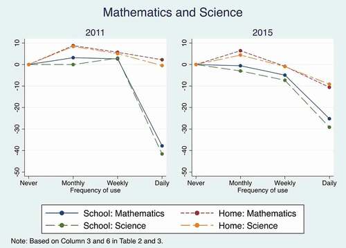
Table 2. Regression on computer use at school and at home and test scores in mathematics and science (2011)

	Mathematics			Science
	1	2	3	4	5	6
School: Monthly	34.55**	6.34**	3.17*	26.15**	2.52	−0.02
	(3.369)	(2.227)	(1.491)	(3.952)	(2.487)	(1.843)
School: Weekly	41.39**	6.19**	2.62	28.11**	6.47**	2.98
	(2.539)	(2.103)	(1.500)	(2.585)	(2.239)	(1.641)
School: Daily	−43.88**	−38.02**	−37.84**	−63.93**	−42.89**	−41.58**
	(4.010)	(2.605)	(2.175)	(4.277)	(3.044)	(2.500)
Home: Monthly	67.17**	13.91**	8.79**	73.59**	13.72**	8.38**
	(3.566)	(2.699)	(2.171)	(4.159)	(3.300)	(2.241)
Home: Weekly	58.36**	12.34**	5.68**	64.80**	12.16**	5.08**
	(2.964)	(2.200)	(1.801)	(3.533)	(2.464)	(1.771)
Home: Daily	51.98**	5.83**	2.23	60.07**	3.52	−0.49
	(3.009)	(2.150)	(1.621)	(3.463)	(2.477)	(1.693)
Background variables	No	Yes	Yes	No	Yes	Yes
Country fixed effects	No	Yes	No	No	Yes	No
School fixed effects	No	No	Yes	No	No	Yes
Observations	440,834	440,834	440,834	440,834	440,834	440,834
R-squared	0.102	0.491	0.637	0.093	0.501	0.638

Never users are selected as the reference group for computer use at school and at home. The regression is performed using the pv-module in Stata by Kevin MacDonald. The dependent variable is the plausible values for mathematics and science, respectively and the standard errors are reported in parentheses. p < 0.05 is represented by * and p < 0.01 by **. Other covariates consist of a set of background variables of the students found in Tables A4 and A5 in the Appendix.

Table 3. Regression on computer use at school and at home and test scores in mathematics and science (2015)

	Mathematics			Science
	1	2	3	4	5	6
School: Monthly	52.99**	0.29	−0.58	41.98**	−2.45	−2.99
	(3.159)	(2.054)	(1.774)	(3.070)	(1.961)	(1.774)
School: Weekly	13.97**	−0.90	−4.93	11.17**	−2.87	−7.32*
	(4.097)	(3.004)	(2.722)	(4.000)	(3.067)	(2.983)
School: Daily	−31.42**	−25.94**	−25.20**	−35.38**	−29.58**	−29.16**
	(5.239)	(3.349)	(3.263)	(5.006)	(2.894)	(2.393)
Home: Monthly	57.33**	12.12**	6.42**	54.69**	11.75**	4.38*
	(3.993)	(2.160)	(2.047)	(4.211)	(2.466)	(1.852)
Home: Weekly	39.99**	7.20**	−0.85	42.49**	8.93**	−0.95
	(3.793)	(2.332)	(2.166)	(4.075)	(2.533)	(2.086)
Home: Daily	23.66**	−6.57**	−10.60**	28.87**	−3.16	−9.15**
	(3.658)	(2.116)	(1.927)	(3.876)	(2.649)	(2.191)
Background variables	No	Yes	Yes	No	Yes	Yes
Country fixed effects	No	Yes	No	No	Yes	No
School fixed effects	No	No	Yes	No	No	Yes
Observations	499,273	499,273	499,273	499,273	499,273	499,273
R-squared	0.074	0.582	0.713	0.066	0.514	0.674

see Table 2.

This section first describes how the results are affected by model specifications, while the second part presents the main results. The final section compares the impact of computers on boys and girls, OECD and non-OECD countries, and low-, median- and high-performing pupils.

In columns 1 and 4, there is an overall significant and positive association between computer use and test scores, except for daily use at school. Monthly users are the highest-performing group of pupils and they achieve up to 74 and 57 points more than never users in 2011 and 2015, respectively. The positive estimates for computer use decline when variables for student background and country fixed effects are added in columns 2 and 5. Estimates for weekly and monthly computer use at school become less positive, and the estimate for daily use is less negative in this specification. Furthermore, the standard errors shrink and the significance decreases for weekly and monthly use at home when background controls are included.

The results reported in columns 2 and 5 with country fixed effects support some of the findings of an inverted u-shape reported by Fuchs and Wössmann (2004). They found that computer use and performance are positively related to monthly users, which declines and become significantly negative for the students who use a computer more than a few times a week. This inverted u-shape is most apparent in school use in 2011. Conversely, in 2015, the u-shape appears for home use (most of all in mathematics) and the positive estimates of school use is insignificant and negative for science.

When country fixed effects are replaced with school fixed effects, the positive estimates of computer use shrink in magnitude and the significance levels become less strong in 2011.⁸ The inverted u-shape, which is observed in a simple model of just computer use, diminishes and almost disappears in the model specification with background controls and school fixed effects.

The regression estimates from columns 3 and 6, with background variables and school fixed effects, are shown in Figure 1 to get an overview of the main result. The estimated test scores are plotted by subject, frequency of use, and location, and the result from the TIMSS wave is reported separately in each graph. There is a consistent and reappearing pattern across years and between subjects: computer use at home is associated with higher achievement than computer use at school and moderate use (monthly and weekly) is associated with higher scores than daily use. Mathematics and science results follow the same patterns. The significance level is not visible in the figure but Tables 2 and 3 report that some of the estimates become insignificant in the main model with school fixed effects. Daily school use is significantly associated with lower test scores for both subjects in both years, but no distinct pattern in significance level appears for the other estimates.

Even if the pattern is consistent between the years, the size of the estimates and the significance levels vary over the waves. In general, computer use and test scores are positively associated with more groups in 2011 than 2015 but the estimates of daily use are more negative in 2011. The negative association is especially distinct for school users, as daily users score around 25–42 points less than never users accordingly to the point estimates. Given that 100 points on the TIMSS scale equal one standard deviation, the estimates are equivalent to 0.25 and 0.40 standard deviations respectively. Except for moderate use in 2011, computer use at school is always negatively associated with test scores, while the result for home computer use is more ambiguous. Moderate use of computers at home shows a small significant positive association with test scores: weekly use is associated with higher test scores in 2011, but not in 2015, and the estimates for monthly users are positive and significant in both years. The largest difference appears for daily computer use at home, as there is a significant negative estimate for daily home users in 2015, while the corresponding groups in 2011 show a zero or small negative association.

The results suggest an overall negative association between computer use in schools and test scores, where the estimated differences among never users and daily users are between 0.25 and 0.4 standard deviations in favour of the never users. In contrast, studies such as Muralidharan et al. (2019) or Hull and Duch (2019) report positive effects of increased computer access on test scores in the size of 0.37 and 0.13 standard deviations, respectively. The estimated associations in this study are more in line with the findings from Carter et al. (2017) who report that students who were allowed to use computers scored 0.18 standard deviations lower than their counterparts. A number of studies did not, however, find any significant impact of computer use on educational outcomes (see, e.g., Beuermann et al., 2015; Falck et al., 2018; Yanguas, 2020).

These results also show the importance of including controls for determinants of the educational production function and support the suggestion that test scores are determined by many factors other than computer use. Inclusion of background controls and school fixed effects changes the estimates significantly, with school fixed effects adjusting for unobserved heterogeneity between different schools. Fuchs and Wössmann (2004) also report a negative association between computer use at school and test scores when it is used frequently (several times a week or more). The size of the negative association is, however, larger in this study. They report that the frequent users achieved 4 points less than never users, while the estimated association for daily users is 41 points in this study. Note that weekly and daily computer use is considered as frequent computer use in the PISA data used by Fuchs & Wössmann. In conclusion, location and frequency of use matters when analysing the impact of computer use on test scores. School use is associated with a lower test score than computer use at home and daily computer use is rarely positively associated with test scores. Even if the negative associations are larger in this study than the findings by Fuchs & Wössmann in absolute terms, a negative association of 0.4 standard deviations is not considerably large in the TIMSS context.

5.1. Subgroup comparisons

The association of computer use and test scores is likely to vary between heterogeneous groups of pupils. Therefore, additional analyses are conducted on subsamples based on gender, OECD membership, and low-, median- and high-performing pupils. The first two analyses use the same method as the main model, while the last comparison uses unconditional quantile regression analysis to determine the impact of computers in different parts of the distribution. The results from the gender and country comparisons are presented in figures and a complete table of regression estimates and their significance levels are found in the Appendix.

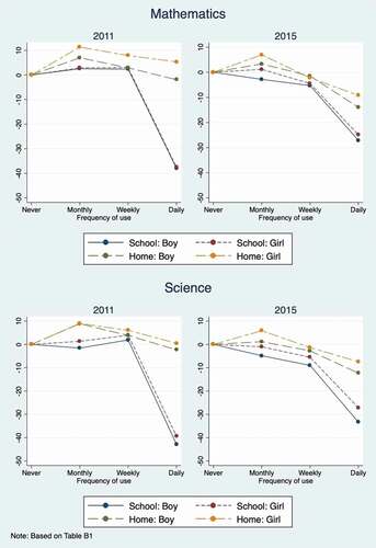
Figure 2 reports the results from the gender comparison. The results are divided into four separate graphs instead of two because of the increased number of reported estimates. The two graphs at the top of the figure show regression estimates for mathematics scores while the bottom graphs illustrate the science results. The comparison of girls and boys by school and home use is visible within each graph. As with the main result, home use is better than school use, and moderate use is still most positively associated with test scores. The trends are almost identical between subjects, showing that the impact of computers is similar for mathematics and science. Computer use at home tends to be more positively associated with test scores for girls than for boys but the gender differences in associations tend to be small. The largest gender difference is observed among home use for mathematics results in 2011, with girls scoring between 3 and 13 points higher in every frequency of use. Overall, there is no clear evidence that one gender benefits more from computer use than the other.

Figure 2. Associations between computer use and test scores in mathematics and science by gender

A country-by-country comparison could be made to analyse heterogeneous effects on country levels (e.g. Spiezia, 2011). Instead, this paper divides the participating countries into OECD and non-OECD countries, assuming that these countries are somewhat homogenous. Nonetheless, descriptive data show that there are no large differences in computer use between the type of countries (see Table A7 in the Appendix).

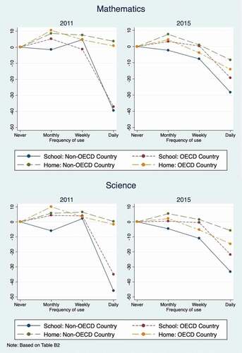
Figure 3 shows regression estimates from a model with background variables and school fixed effects on subsamples of OECD and non-OECD countries. The figure reports the subject and year in separate graphs to highlight country differences. There is an overall positive association between monthly use and test scores. Daily use and test scores are negatively associated and in both groups of countries and computer use in schools are more negatively associated with test scores, although the result of country differences is somewhat ambiguous. The trend lines for school use in OECD countries are almost always above the non-OECD group, indicating that computer use in schools is less negatively associated with test scores in OECD countries than in non-OECD countries. The result is, more or less the opposite for home users. The test scores in non-OECD countries are also more positively associated with all frequencies of computer use at home than OECD countries in 2015, but only for more frequent use (weekly and daily) in 2011.

Figure 3. Associations between computer use and test scores in mathematics and science test scores by OECD membership

The final part of this analysis focuses on the impact of computers on different points of the test score distribution. Do the associations between computer use and test scores differ between low-, middle- and high-performing pupils? An unconditional quantile regression (UQR) is applied to analyse how associations vary along with the test score distribution. School weights are used instead of student weights and only the first plausible value for each subject is used as the dependent variable. Also, the standard errors are robust and clustered at school level.⁹ The estimates from the UQR should not be directly compared to the pv-regression as the model differs in weights and the application of plausible values. However, comparing the results presented in columns 3 and 6 in Tables 2 and 3 with those in Table B3 in the Appendix, where OLS regression with the same weights and robust standard errors as in the UQR is used, indicates that the difference in weights and application of plausible values only have a small impact on the estimates.

Tables 4 and 5 show that the relationship of computer use at school and test scores varies between quantiles. Background controls and school fixed effects are included in all the regressions. Each quantile of the test score distribution is represented by one column. The result is in line with the previous findings that daily use in school is negatively related to test scores. Here the same is found for daily use in both years, both subjects, and across all percentiles. In 2011, for example, a pupil in the 10th percentile who used a computer every day performs 62 points less in mathematics than a non-user. The estimate of daily computer use is, by contrast, less negative in the 90th percentile: a pupil in the 90th percentile only achieved 12 points less than a pupil who never used a computer in school. The same pattern for daily use also appears for the science scores in 2011 and both subjects in 2015. The results also show that all computer use in school is negatively associated with test scores for low-performing students. For both subjects and years, the associations are negative for all frequencies in the 10th percentile, and the associations are significant except for monthly use in 2015. Furthermore, the standard errors are larger in the lower part of the distribution, indicating that the estimates are less precise. The estimates in the 50th and 90th percentile are in most cases positive and significant but small in size.

Table 4. Unconditional quantile regression on computer use at school and at home and test scores in mathematics and science 2011

	Mathematics			Science
	10^th percentile	50^th percentile	90^th percentile	10^th percentile	50^th percentile	90^th percentile
School: Monthly	−5.48	3.28	10.00**	−5.43	2.99	4.19
	(4.146)	(1.977)	(2.392)	(4.291)	(2.084)	(2.500)
School: Weekly	−9.23*	0.24	8.96**	−7.86	2.18	6.46**
	(4.282)	(1.963)	(2.078)	(4.709)	(2.057)	(2.342)
School: Daily	−62.39**	−35.65**	−12.11**	−71.52**	−38.94**	−12.20**
	(7.965)	(2.803)	(2.380)	(9.530)	(2.961)	(3.350)
Home: Monthly	16.00*	9.50**	5.65	12.62*	10.06**	6.99*
	(6.571)	(3.024)	(3.373)	(6.144)	(3.108)	(3.453)
Home: Weekly	11.24*	6.60**	1.06	8.95	6.02*	−1.29
	(5.722)	(2.289)	(2.376)	(6.029)	(2.466)	(2.413)
Home: Daily	4.77	4.20*	−2.14	−0.54	2.39	−0.64
	(5.349)	(2.319)	(2.557)	(6.050)	(2.504)	(2.566)
Background variables	Yes	Yes	Yes	Yes	Yes	Yes
School fixed effects	Yes	Yes	Yes	Yes	Yes	Yes
Observations	440,834	440,834	440,834	440,834	440,834	440,834
No of schools	6,245	6,245	6,245	6,245	6,245	6,245

Never users are selected as the reference group for computer use at school and at home. The dependent variable is the first plausible value for mathematics and science, respectively. The standard errors are reported in the parentheses and clustered at school level. p < 0.05 is represented by * and p < 0.01 by **. Other covariates consist of a set of background variables of the students found in Tables A4 and A5 in the Appendix.

Table 5. Unconditional quantile regression on computer use at school and at home and test scores in mathematics and science 2015

	Mathematics			Science
	10^th percentile	50^th percentile	90^th percentile	10^th percentile	50^th percentile	90^th percentile
School: Monthly	−15.64**	5.22*	3.09	−16.44**	3.93	3.04
	(4.212)	(2.285)	(3.926)	(4.719)	(2.189)	(3.004)
School: Weekly	−23.04**	0.79	−1.86	−34.36**	1.65	−0.59
	(5.737)	(2.992)	(2.186)	(9.884)	(2.595)	(2.266)
School: Daily	−58.02**	−21.20**	−11.50**	−56.21**	−29.36**	−12.40**
	(11.22)	(2.791)	(2.282)	(8.483)	(2.729)	(2.176)
Home: Monthly	7.09	5.72*	3.60	6.02	1.98	5.37*
	(7.215)	(2.446)	(3.527)	(6.079)	(2.471)	(2.565)
Home: Weekly	6.07	−1.09	−13.91**	2.58	−3.88	−7.56**
	(5.065)	(2.382)	(2.500)	(6.246)	(2.242)	(2.142)
Home: Daily	−2.10	−14.16**	−19.28**	−6.25	−12.16**	−14.02**
	(5.778)	(2.463)	(2.426)	(6.413)	(2.283)	(1.823)
Background variables	Yes	Yes	Yes	Yes	Yes	Yes
School fixed effects	Yes	Yes	Yes	Yes	Yes	Yes
Observations	499,273	499,273	499,273	499,273	499,273	499,273
No of schools	8,815	8,815	8,815	8,815	8,815	8,815

See Table 4.

The results from computer use at school do not apply to computer use at home. The pupils who benefit most from computer use at home are in the 10th or 50th percentile. Overall, computer use at home is more associated with a positive impact on test scores in 2011 than in 2015, at least when a computer is used monthly or weekly. Daily computer use and test scores are in most cases negatively associated for both high- and low-achieving pupils. Still, the negative association is not as large as for daily computer use at school. The size of the largest negative estimate is −19 points compared to estimates of −72 points in daily school use.

In conclusion, the results show that the estimates for computer use vary in different parts of the test score distribution, suggesting that the association between computer use at school and test scores is more negative among low-performing pupils than high-performing pupils. Daily computer use at school is negatively associated with test scores, but the negative association is smaller among high-achieving pupils. This does not hold for computer use at home, where the estimates in the middle and lower end of the score distribution are more positively associated with computer use. The test scores in the 90th percentile also positively associated with monthly computer use and the negative association is most evident in weekly and daily home use in 2015.

6. Conclusion

This paper examines the relationship between computer use and test scores among 10-year-old pupils in TIMSS 2011 and 2015. It analyses the impact of computers by including a large set of background controls for determinants that influence pupils’ performance, as well as school fixed effects to control for unobserved heterogeneity between schools. This study finds little evidence that there is a positive association between computer use in schools and pupils’ learning, except in 2011 for moderate use and among high-performing pupils. Monthly and weekly computer use is positively associated with test scores but the associations are most times weak. The results could be affected by selection, but given the extensive controls the results can be seen as a piece of evidence suggesting that one cannot simply implement computers in education and expect the achievement to increase. Consistent with previous studies (see e.g. Beuermann et al., 2015; Carter et al., 2017; Yanguas, 2020), this study finds mostly no or weak evidence that computers in education are increasing achievement. The evidence for positive effects of using computers reported in previous studies (e.g. Barrow et al., 2009; Muralidharan et al., 2019) is limited to cases when computers have been implemented in aided computer sessions and even then, the size of the positive effects are relatively small. The results of this paper also suggest that daily use of computers in school might affect test scores negatively, if computers are used as they were used in 2011 and 2015.

The relationship between computers and test scores varies by frequency of use and location. School use is more negatively associated with test scores than home use, with some groups achieving 70 points (about 0.7 standard deviations) less than pupils who never use a computer. On the other hand, if computers are used at moderate amounts, the performance is positively related to home use. The estimated positive relation is however small. Analysis of gender and country subsamples show similar trends, with gender and country seeming to matter relatively little.

More interesting is that the association between computer use at school and test scores varies in different parts of the test score distribution. The results show larger negative estimates of computer use at school among low-performing pupils than high-performing pupils, while the opposite holds for home use. The positive relation of home use for the bottom of the distribution is, however, not large and are non-significant in many cases. Overall, the test score estimates are many times not larger than ten points, which in a TIMSS context corresponds to 0.10 of a standard deviation of the test score distribution. Even if the observed difference is not substantial, there is a distinct pattern of frequent use of computers in school being negatively associated with test scores, especially among low- and median performing students.

The positive association of computer use at home is weaker in this paper than in previous studies that utilised similar methods but on older pupils. The inclusion of school fixed effects seems to be a reason for the observed results. A contributing explanation can be that fourth graders do not benefit from computers in the same way as eighth graders. Pupils at this age may need training with traditional methods to get the basic knowledge that will allow them to use a computer more efficiently later in their education. Another explanation of the results might be that the distraction effect is more important among young pupils. It might be so that younger pupils are more likely to use the computers for entertainment purposes rather than educational activities, as Beuermann et al. (2015) observed.

Note that the focus of this paper is the associations between computer and test scores, not the potential of computers. The results report a negative association of daily computer use and test scores given how computers were used in 2011 and 2015. What is shown in this study is that computer use at schools was generally associated with lower test scores in mathematics and science, but the results do not provide causal evidence on the effect of computers in education. The findings from this study do not, however, reject that computers have a positive impact on educational achievement if computers are optimally implemented. Therefore, the result is not in conflict with the result from studies that evaluate the effect of computers by studying one-to-one laptop programmes or computer sessions guided by teachers. The results from this study reflect the actual computer use by pupils, which is perhaps the explanation why the results are more in line with studies that analyse the impact of increased computer access rather than the effect from guided computer sessions.

Future studies could focus on finding methods to estimate the causal effect of computer use on achievement when the computers are implemented on a larger scale or investigate the difference between simply increasing computer access and increasing the computer access within a monitored programme. It would also be interesting to determine the role of computers in other subjects than mathematics and science.

Acknowledgments

The author would like to thank Tomas Raattamaa, Olle Westerlund, David Granlund, Magnus Wikström, Nafsika Alexiadou and two anonymous referees for helpful comments and suggestions. Financial support by Handelsbanken (ref. P2016-0299) is gratefully acknowledged.

Disclosure statement

No potential conflict of interest was reported by the author.

Additional information

Funding

This work was supported by the Handelsbanken [P2016-0299].

Notes on contributors

Linn Karlsson

Linn Karlsson is a PhD student at Umeå University, where she furthers her research in Economics of Education. Her interests include ICT in education, admissions and adult education.

Notes

1. The impact of computer use and education have been investigated by a number of other studies. See, e.g. Banerjee, Cole, Duflo, and Linden (2007), Cristia, Ibarrarán, Cueto, Santiago, and Severín (2012), Leuven, Lindahl, Oosterbeek, and Webbink (2007), Machin, McNally, and Silva (2007) and Spiezia (2011).

2. It is important to make a distinction between causal and non-causal relationships. Non causal relationships mistaken for causal effects can lead to false or misleading conclusions, such as described by DiNardo and Pischke (1997).

3. Pupils with special needs are excluded from the TIMSS study in the sampling process. Special needs pupils include children with physical, mental or severe learning disabilities (LaRoche, Joncas, & Foy, 2016).

4. See Foy et al. (2015) for a detailed description of plausible values and how to apply plausible values in regression analysis.

5. For example, a student is considered with many resources if there are at least 100 books and 25 children books at home and at least one parent with a university degree and a professional occupation.

6. Pv is a module in Stata written by Kevin Macdonald and is designed to estimate large-scale international assessments with plausible values. For further description of the module, see (Macdonald, 2008).

7. TIMSS uses a two-stage cluster design which allows the regression errors to be correlated within schools and within classes. Appropriate weights and variance estimation techniques (such as jackknife repeated replication) are required to get accurate point estimates and standard errors (LaRoche et al., 2016).

8. The computer estimates between the model specification with country fixed effects and school fixed effects are tested for significant differences. Of the 24 estimates for computer use, 16 are significantly affected by using school fixed effects instead of country fixed effects. The estimates that are not statistically different at p < 0.05 are daily and monthly computer use for both subjects and both years.

9. The stata command xtrifreg allows unconditional quantile regression (UQR) with a large number of fixed effects. It does not support the use of several plausible values or student weights. It was written by Borgen (2016) and is a version of the UQR developed by Firpo et al. (2009). See Killewald and Bearak (2014) for a formal econometric description.

Appendix A.

Table A1. Questionnaire questions

Year	Question code	Question	Answers
2011		How often do you use the computer in each of these places? a)At home b)At school	1.Every day or almost every day 2.Once or twice a week 3.Once or twice a month 4.Never or almost never
2015		How often do you use a computer or tablet in each of these places for schoolwork (including classroom tasks, homework, studying outside of class)? a)At home b)At school	1.Every day or almost every day 2.Once or twice a week 3.Once or twice a month 4.Never or almost never

Table A2. Missing values in each variable

	2011		2015
Variable	Missing	Percent Missing	Missing	Percent Missing
Computer use at home	24,582	3.82	33,413	4.41
Computer use at school	37,644	5.85	31,619	4.18
Student age	1,550	0.24	509	0.07
Student gender	10	0	169	0.02
Country of birth	-	-	31,155	4.12
Parent highest education	89,007	13.84	126,567	16.72
Father working status	110,319	17.16	143,883	19.01
Father occupation	144,772	22.51	179,864	23.76
Mother working status	152,833	23.77	181,288	23.95
Mother occupation	169,670	26.38	196,291	25.93
Books at home	59,631	9.27	108,263	14.30
Years been teaching	56,780	8.83	52,596	6.95
Teacher gender	37,788	5.88	32,913	4.35
Teacher’s education	42,277	6.57	80,974	10.70
	n = 643,066		n = 757,026

Number of missing values for each variable. Bold text indicates categorical variables.

Table A3. Participating countries in TIMSS 2011 and 2015

Countries		TIMSS 2011	TIMSS 2015	Countries	TIMSS 2011	TIMSS 2015
Abu Dhai		x	x	Italy	x	x
Australia		x		Japan	x	x
Austria			x	Kazakhstan		x
Azerbaijan			x	Rep. of Korea		x
Bahrain		x	x	Kuwait		x
Belgium (Flemish)			x	Lebanon	x	x
Botswana		x	x	Lithuania	x
Buenos Aires			x	Malaysia	x	x
Bulgaria		x	x	Malta	x	x
Canada		x	x	Morocco		x
Canada (Quebec)			x	Netherlands	x	x
Canada (Ontario)		x	x	New Zealand	x	x
Chile			x	North Ireland	x	x
Chinese Taipei		x	x	Norway	x	x
Croatia			x	Oman	x	x
Cyprus		x	x	Poland	x	x
Czech Republic		x	x	Portugal		x
Denmark		x		Qatar		x
Dubai		x	x	Romania	x
England		x*	x*	Russia	x	x
Finland			x	Saudi Arabia	x	x
France		x	x	Serbia		x
Georgia		x	x	Singapore	x	x
Germany		x	x	Slovak Rep.	x	x
Honduras		x		Slovenia	x	x
Hong Kong			x	Spain	x	x
Hungary			x	Sweden	x	x
Indonesia		x	x	Turkey		x
Iran			x	United Arab Emirates	x	x
Ireland		x	x	United States		x*

Countries included in TIMSS database for 4^th grade. OECD countries (in 2011 and 2015) are in bold. England and United States are indexed with * and are excluded from the analysis due to missing information in the home questionnaire. There are 35 and 48 countries included in TIMSS 2011 and 2015 respectively.

Table A4. Categorical variables

Variable	2011	2015
Computer use at home
Every day	47.82	38.24
Weekly	35.11	28.32
Monthly	7.41	14.02
Never	9.66	19.41
Computer use at school
Every day	7.91	11.30
Weekly	45.97	27.34
Monthly	14.98	13.94
Never	31.14	47.42
Gender
Girl	50.44	50.52
Boy	49.56	49.48
Were you born in the test country?
Yes	-	86.41
No	-	13.59
Resources at home for education*
Many resources	15.63	19.24
Some resources	76.59	73.04
Few resources	7.78	5.72
No-response	-	2.00
Parent highest education
University or higher	35.77	42.66
Post-secondary	17.76	19.83
Upper Secondary	27.85	22.28
Lower Secondary	11.47	5.86
Some primary or no school	6.91	5.39
Not applicable	0.23	0.52
No-response	-	3.39
Father working status
At least full-time	70.16	73.20
Part-time	8.07	6.97
Not working for pay	3.91	3.14
Other	7.93	7.38
Not applicable	4.03	3.58
No response	5.91	5.73
Father occupation
Never worked	1.92	1.48
Business	10.73	10.94
Clerk	7.04	5.96
Service	9.27	8.54
Agricultural	1.96	1.84
Craft/Trade	10.00	9.29
Plant Op	6.49	6.74
Labourers	3.57	4.76
Manager	11.45	12.18
Professional	12.51	13.64
Technician	5.83	6.34
Not applicable	8.34	7.74
No response	10.88	10.54
Mother working status
At least full-time	37.44	42.05
Part-time	12.36	14.24
Not working for pay	14.52	13.70
Other	7.93	7.71
Not applicable	15.02	11.79
No-response	12.73	10.51
Mother occupation
Never worked	13.32	10.23
Small Business	4.43	5.44
Clerk	11.65	12.10
Service or Sales	9.67	10.35
Skilled Agricultural or fishery	0.68	0.67
Craft or Trade	1.30	1.30
Plant or Machine operator	1.87	1.65
Labourers	3.30	3.89
Manager	3.47	4.89
Professional	13.76	16.47
Technician	5.35	6.12
Not applicable	16.11	14.22
No response	15.10	12.68
Books at home
0–10	19.08	21.46
11–25	21.17	21.08
26–100	31.48	30.12
101–200	12.12	12.23
200 or more	16.14	15.11
Teacher gender
Female	83.48	81.90
Male	16.52	18.10
Teacher’s education
Did not complete upper secondary	0.41	0.32
Upper secondary	4.89	3.34
Post-secondary	5.57	2.43
Short-cycle teritary	8.23	7.07
Bachelor’s or equivalent	57.38	59.79
Master’s or equivalent	23.52	26.49
Doctor’s or equivalent	-	0.56
Total	N = 440,834	N = 499,273

Table of categorical variables. All variables except resources at home for education are included in the model since resources at home is already accounted for by parental background and number of books at home.

Table A5. Continuous variables

	2011		2015
	Mean	Standard deviation	Mean	Standard deviation
Test score
Mathematics	479.68	1.59	488.00	2.21
Science	486.18	1.66	488.36	2.37
Student/School/Teacher variables
Student age	10.08	0.54	10.10	0.54
Years been teaching	15.66	10.36	15.80	10.58
Total	n = 440,834		n = 499,273

Table of continuous variables in the model.

Table A6. Resources at home and computer use

	Computer use at home				Computer use at school
2011	Daily	Weekly	Monthly	Never	Daily	Weekly	Monthly	Never
Many Resources	47.58	39.54	9.10	3.77	4.99	45.54	20.26	29.21
Some Resources	49.71	35.24	7.13	7.93	8.21	46.44	14.4	30.95
Few Resources	29.68	25.01	6.76	38.56	10.79	42.25	10.01	36.95
2015	Daily	Weekly	Monthly	Never	Daily	Weekly	Monthly	Never
Many Resources	34.19	30.98	17.67	17.16	10.64	29.79	17.7	41.86
Some Resources	39.91	28.32	13.49	18.27	11.27	26.88	13.41	48.44
Few Resources	28.46	20.37	10.04	41.13	12.88	23.53	9.26	54.33
Missing	44.12	25.7	9.62	20.56	14.52	31.34	10.37	43.76

Cross-tabulation of resources at home and computer use in percentage.

Table A7. OECD membership and computer use

	Computer use at home				Computer use at school
2011	Daily	Weekly	Monthly	Never	Daily	Weekly	Monthly	Never
Non-OECD	46.97	34.83	6.72	11.47	8.85	50.02	11.41	29.71
OECD	49.61	35.71	8.85	5.84	5.92	37.39	22.52	34.17
2015	Daily	Weekly	Monthly	Never	Daily	Weekly	Monthly	Never
Non-OECD	40.33	28.45	12.84	18.38	11.55	27.97	13.02	47.46
OECD	35.35	28.14	15.66	20.84	10.96	26.47	15.21	47.35

Cross-tabulation of OECD, non-OECD country and computer use in percentage.

Table A8. Gender and computer use

	Computer use at home				Computer use at school
2011	Daily	Weekly	Monthly	Never	Daily	Weekly	Monthly	Never
Girl	43.59	38.31	8.14	9.96	6.65	46.7	14.97	31.68
Boy	52.12	31.86	6.66	9.36	9.19	45.23	14.98	30.60
2015	Daily	Weekly	Monthly	Never	Daily	Weekly	Monthly	Never
Girl	36.15	30.58	14.57	18.70	10.49	28.11	13.94	47.46
Boy	40.38	26.02	13.46	20.13	12.13	26.56	13.94	47.38

Cross-tabulation of gender and computer use in percentage.

Table A9. Correlation between computer use in school and at home

Computer use at school	Computer use at home
2011	Daily	Weekly	Monthly	Never
Daily	62.42	25.78	4.7	7.1
Weekly	50.02	35.75	6.77	7.46
Monthly	42.71	41.52	8.35	7.42
Never	43.32	33.46	8.57	14.65
2015	Daily	Weekly	Monthly	Never
Daily	58.38	24.53	7.18	9.91
Weekly	42.96	31.60	13.2	12.23
Monthly	31.51	32.93	19.07	16.49
Never	32.80	25.91	14.59	26.70

Cross-tabulation of computer use at school and at home. Each row shows the share (in per cent) of computer use at home by each category of school use.

Appendix B.

Table B1. Gender-specific regressions

	2011		2015
Mathematics	Boy	Girl	Boy	Girl
School: Monthly	2.533	2.889	−2.835	1.152
	(2.093)	(2.179)	(2.428)	(2.732)
School: Weekly	2.352	2.965	−5.314	−4.473
	(2.002)	(2.605)	(3.598)	(3.022)
School: Daily	−37.961**	−37.498**	−27.116**	−24.919**
	(2.724)	(3.738)	(4.415)	(3.572)
Home: Monthly	6.989*	11.330**	3.298	6.924*
	(3.302)	(2.233)	(2.424)	(2.787)
Home: Weekly	2.893	7.889**	−1.476	−2.225
	(2.980)	(1.922)	(2.336)	(2.932)
Home: Daily	−1.910	5.332**	−13.963**	−9.218**
	(2.960)	(1.849)	(2.455)	(2.368)
Background Variables	Yes	Yes	Yes	Yes
School fixed effects	Yes	Yes	Yes	Yes
Observations	218,484	222,350	247,055	252,218
R-squared	0.659	0.651	0.737	0.734
Science	2011		2015
	Boy	Girl	Boy	Girl
School: Monthly	−1.562	1.329	−4.855	−1.046
	(2.464)	(2.466)	(2.606)	(3.324)
School: Weekly	1.904	3.936	−9.005*	−5.515
	(2.204)	(2.288)	(4.030)	(3.339)
School: Daily	−42.829**	−39.382**	−33.329**	−27.196**
	(2.792)	(4.129)	(3.502)	(4.005)
Home: Monthly	8.865*	8.962**	1.161	5.859
	(3.491)	(2.758)	(2.682)	(3.002)
Home: Weekly	3.822	6.038*	−2.758	−1.338
	(2.971)	(2.712)	(3.149)	(3.090)
Home: Daily	−2.346	0.479	−12.318**	−7.457*
	(2.692)	(2.329)	(3.238)	(3.229)
Background Variables	Yes	Yes	Yes	Yes
School fixed effects	Yes	Yes	Yes	Yes
Observations	218,484	222,350	247,055	252,218
R-squared	0.669	0.643	0.696	0.690

Never users are selected as the reference group for computer use at school and at home. The regression is performed using the pv-module in Stata by Kevin MacDonald. The dependent variable is the plausible values for mathematics and science, respectively and the standard errors are reported in parentheses. p < 0.05 is represented by * and p < 0.01 by **. Other covariates consist of a set of background variables of the students found in Tables A4 and A5 in the Appendix.

Table B2. OECD and non-OECD country regressions

	2011		2015
Mathematics	Non-OECD	OECD	Non-OECD	OECD
School: Monthly	−1.548	5.183**	−2.360	3.117*
	(2.625)	(1.505)	(2.572)	(1.252)
School: Weekly	4.738*	−1.342	−7.649	0.291
	(1.947)	(1.441)	(3.941)	(1.285)
School: Daily	−39.441**	−37.102**	−28.294**	−19.415**
	(2.761)	(2.502)	(4.768)	(1.906)
Home: Monthly	8.561**	10.511**	7.564*	4.242**
	(2.934)	(2.414)	(2.998)	(1.393)
Home: Weekly	7.605**	4.588*	0.987	−3.916**
	(2.249)	(2.009)	(3.252)	(1.200)
Home: Daily	3.681*	0.834	−8.290**	−14.185**
	(2.103)	(1.968)	(3.050)	(1.032)
Background Variables	Yes	Yes	Yes	Yes
School fixed effects	Yes	Yes	Yes	Yes
Observations	299,446	141,388	290,065	209,208
R-squared	0.680	0.393	0.748	0.497
Science	2011		2015
	Non-OECD	OECD	Non-OECD	OECD
School: Monthly	−5.944	4.330*	−4.603	0.436
	(3.400)	(1.971)	(2.518)	(1.274)
School: Weekly	2.173	3.959*	−11.058*	−0.561
	(2.522)	(1.947)	(4.525)	(1.028)
School: Daily	−45.832**	−34.960**	−33.229**	−21.791**
	(3.990)	(3.023)	(3.430)	(2.009)
Home: Monthly	5.762	10.049**	5.412*	2.179
	(3.399)	(3.225)	(2.694)	(1.493)
Home: Weekly	6.458**	3.338	1.521	−5.386**
	(2.289)	(2.726)	(3.030)	(1.305)
Home: Daily	0.316	−1.693	−5.824	−14.658**
	(2.160)	(2.961)	(3.295)	(1.087)
Background Variables	Yes	Yes	Yes	Yes
School fixed effects	Yes	Yes	Yes	Yes
Observations	299,446	141,388	290,065	209,208
R-squared	0.666	0.385	0.688	0.460

See Table B1.

Table B3. Standard OLS regression

	2011		2015
	Mathematics	Science	Mathematics	Science
School: Monthly	3.577**	−0.121	−0.037	−2.494**
	(0.779)	(0.809)	(0.846)	(0.849)
School: Weekly	−0.044	0.458	−5.792**	−7.641**
	(0.774)	(0.803)	(0.899)	(1.012)
School: Daily	−37.349**	−40.812**	−27.257**	−30.071**
	(1.109)	(1.209)	(1.194)	(1.199)
Home: Monthly	10.246**	9.215**	5.848**	3.678**
	(1.121)	(1.229)	(0.943)	(0.979)
Home: Weekly	6.273**	5.697**	−2.515**	−2.514**
	(0.913)	(0.952)	(0.901)	(0.936)
Home: Daily	3.344**	1.310	−11.201**	−10.138**
	(0.913)	(0.952)	(0.865)	(0.929)
Background Variables	Yes	Yes	Yes	Yes
School fixed effects	Yes	Yes	Yes	Yes
Observations	440,834	440,834	499,273	499,273
R-squared	0.615	0.630	0.697	0.656

Never users are selected as the reference group for computer use at school and at home. Dependent variable is the first plausible value. Regression includes school weights and robust standard errors are clustered at school level.

References

- Banerjee, A. V., Cole, S., Duflo, E., & Linden, L. (2007). Remedying education: Evidence from two randomized experiments in India. The Quarterly Journal of Economics, 122(3), 1235–1264.
- Barrow, L., Markman, L., & Rouse, C. E. (2009). Technology’s Edge: The Educational Benefits of Computer-Aided Instruction. American Economic Journal: Economic Policy, 1(1), 52–74.
- Bedard, K., & Dhuey, E. (2006). The persistence of early childhood maturity: International evidence of long-run age effects. The Quarterly Journal of Economics, 121(4), 1437–1472.
- Beuermann, D. W., Cristia, J., Cueto, S., Malamud, O., & Cruz-Aguayo, Y. (2015). One laptop per child at home: Short-term impacts from a randomized experiment in Peru. American Economic Journal: Applied Economics, 7(2), 53–80.
- Black, S. E., Devereux, P. J., & Salvanes, K. G. (2011). Too young to leave the nest? The effects of school starting age. The Review of Economics and Statistics, 93(2), 455–467.
- Borah, B. J., & Basu, A. (2013). Highlighting differences between conditional and unconditional quantile regression approaches through an application to assess medication adherence. Health Economics, 22(9), 1052–1070.
- Borgen, N. T. (2016). Fixed effects in unconditional quantile regression. The Stata Journal: Promoting communications on statistics and Stata, 16(2), 403–415.
- Bulman, G. and R. W. Fairlie (2016), “Technology and education: Computers, software, and the internet” in Hanushek, E. A., S. Machin and L. Woessman (eds.), Handbook of the Economics of Education, Elsevier, Amsterdam.
- Carter, S. P., Greenberg, K., & Walker, M. S. (2017). The impact of computer usage on academic performance: Evidence from a randomized trial at the United States Military Academy. Economics of Education Review, 56, 118–132.
- Cascio, E. U., & Schanzenbach, D. W. (2016). First in the class? Age and the education production function. Education Finance and Policy, 11(3), 225–250.
- Cristia, J., Ibarrarán, P., Cueto, S., Santiago, A., & Severín, E. (2012). Technology and child development: Evidence from the one laptop per child program. American Economic Journal: Applied Economics, 9(3), 295-320. Chicago.
- Dickerson, A., McIntosh, S., & Valente, C. (2015). Do the maths: An analysis of the gender gap in mathematics in Africa. Economics of Education Review, 46, 1–22. doi:https://doi.org/10.1016/j.econedurev.2015.02.005
- DiNardo, J. E., & Pischke, J.-S. (1997). The returns to computer use revisited: Have pencils changed the wage structure too? The Quarterly Journal of Economics, 112(1), 291–303.
- Dustmann, C., Frattini, T., & Lanzara, G. (2012). Educational achievement of second-generation immigrants: An international comparison. Economic Policy, 27(69), 143–185.
- Falck, O., Mang, C., & Wössmann, L. (2018). Virtually no effect? Different uses of classroom computers and their effect on student achievement. Oxford Bulletin of Economics and Statistics, 80(1), 1–38.
- Fiorini, M. (2010). The effect of home computer use on children’s cognitive and non-cognitive skills. Economics of Education Review, 29(1), 55–72.
- Firpo, S., Fortin, N. M., & Lemieux, T. (2009). Unconditional quantile regressions. Econometrica, 77(3), 953–973.
- Foy, P., Martin, M. O., Mullis, I. V. S., Yin, L., Cotter, K., & Liu, J. (2015). Reviewing the TIMSS Advanced 2015 Achievement Item Statistics. In Methods and Procedures in TIMSS Advanced 2015 (pp. 11.1–11.19). Retrieved from https://timssandpirls.bc.edu/publications/timss/2015-a-methods/chapter-11.html
- Fredriksson, P., & Öckert, B. (2014). Life-cycle Effects of Age at School Start. The Economic Journal, 124(579), 977–1004.
- Fryer Jr, R. G., & Levitt, S. D. (2010). An empirical analysis of the gender gap in mathematics. American Economic Journal:Applied Economics, 2(2), 210–240.
- Fuchs, T., & Wössmann, L. (2004). Computers and student learning: Bivariate and multivariate evidence on the availability and use of computers at home and at school. Brussels Economic Review, 2004(47), 359–386.
- Hall, Caroline & Lundin, Martin & Sibbmark, Kristina, 2019. “A laptop for every child? The impact of ICT on educational outcomes,„ Working Paper Series 2019:26, IFAU - Institute for Evaluation of Labour Market and Education Policy.
- Hanushek, E. A. (1979). Conceptual and empirical issues in the estimation of educational production functions. The Journal of Human Resources, 14(3), 351–388.
- Hattie, J. (2009). Visible learning: A synthesis of over 800 meta-analyses relating to achievement. Routledge.
- Hernandez, D. J. (2011). Double Jeopardy: How Third-Grade Reading Skills and Poverty Influence High School Graduation. Annie E. Casey Foundation.
- Hull, M., & Duch, K. (2019). One-to-One technology and student outcomes: Evidence from Mooresville’s digital conversion initiative. Educational Evaluation and Policy Analysis, 41(1), 79–97.
- Jerrim, J., Lopez-Agudo, L. A., Marcenaro-Gutierrez, O. D., & Shure, N. (2017). What happens when econometrics and psychometrics collide? An example using the PISA data. Economics of Education Review, 61, 51–58.
- Killewald, A., & Bearak, J. (2014). Is the motherhood penalty larger for low-wage women? A comment on quantile regression. American Sociological Review, 79(2), 350–357.
- LaRoche, S., Joncas, M., & Foy, P. (2016). Sample Design in TIMSS 2015. In Methods and Procedures in TIMSS 2015 (pp. 3.1–3.37). Retrieved from http://timss.bc.edu/publications/timss/2015-methods/chapter-3.html
- Leuven, E., Lindahl, M., Oosterbeek, H., & Webbink, D. (2007). The effect of extra funding for disadvantaged students on achievement. The Review of Economics and Statistics, 89(4), 721–736.
- Kevin Macdonald, 2008. “PV: Stata module to perform estimation with plausible values,„ Statistical Software Components S456951, Boston College Department of Economics, revised 03 Feb 2019.
- Machin, S., McNally, S., & Silva, O. (2007). New Technology in Schools: Is There a Payoff? The Economic Journal, 117(522), 1145–1167.
- Mühlenweg, A. M., & Puhani, P. A. (2010). The evolution of the school-entry age effect in a school tracking system. Journal of Human Resources, 45(2), 407–438.
- Mullis, I.V.S. & Martin, M.O. (Eds.) (2013). TIMSS 2015 Assessment Frameworks. Retrieved from Boston College, TIMSS & PIRLS International Study Center website: http://timssandpirls.bc.edu/timss2015/frameworks.html.
- Martin, M. O., Mullis, I. V. S., & Hooper, M. (Eds.). (2016). Methods and Procedures in TIMSS 2015. Retrieved from Boston College, TIMSS & PIRLS International Study Center website: http://timssandpirls.bc.edu/publications/timss/2015-methods.html.
- Muralidharan, K., Singh, A., & Ganimian, A. J. (2019). Disrupting education? Experimental evidence on technology-aided instruction in India. American Economic Review, 109(4), 1426–1460.
- Organisation for Economic Co-operation and Development. (2006). Are students ready for a technology-rich world?: What PISA studies tell us. OECD Publishing.
- Organisation for Economic Co-operation and Development. (2010). Are the New Millennium Learners Making the Grade?: Technology Use and Educational Performance in PISA 2006. OECD Publishing.
- Robinson, J. P., & Lubienski, S. T. (2011). The development of gender achievement gaps in mathematics and reading during elementary and middle school: Examining direct cognitive assessments and teacher ratings. American Educational Research Journal, 48(2), 268–302. doi:https://doi.org/10.3102/0002831210372249
- Rodríguez-Planas, N., & Nollenberger, N. (2018). Let the girls learn! It is not only about math… it's about gender social norms. Economics of Education Review, 62, 230–253. doi:https://doi.org/10.1016/j.econedurev.2017.11.006
- Schütz, G., Ursprung, H. W., & Wössmann, L. (2008). Education policy and equality of opportunity. Kyklos, 61(2), 279–308.
- Spiezia, V. (2011). Does Computer Use Increase Educational Achievements? Student-level Evidence from PISA. OECD Journal: Economic Studies, 2010(1), 1–22.
- Von Davier, M., Gonzalez, E., & Mislevy, R. (2009). What are plausible values and why are they useful. IERI Monograph Series, 2(1), 9–36.
- Wössmann, L. (2016). The Importance of School Systems: Evidence from International Differences in Student Achievement. Journal of Economic Perspectives, 30(3), 3–32.
- Wu, M. (2005). The role of plausible values in large-scale surveys. Studies in Educational Evaluation, 31(2–3), 114–128.
- Yanguas, M. L. (2020). Technology and educational choices: Evidence from a one-laptop-per-child program. Economics of Education Review, 76, 101984.