Ship acceleration motion under the action of a propulsion system: a combined empirical method for simulation and optimisation

Abstract

The current paper presents a simple mathematical model for replication of the transient acceleration motion of displacement hulls in calm water under the action of a propulsion system. Different empirical methods are coupled, and an operational speed problem is solved in the time domain. The resistance of the ship is calculated by using the Holtrop method. The values of thrust force, torque and propeller efficiency are computed by using B-Series empirical equations. The acceleration motion of the vessel, which is triggered as the engine starts to work, is simulated by solving a set of first-order differential equations, which are discretised in the time domain. It is shown that different propellers can lead to different transient and steady behaviours of the vessel. Finally, using a genetic algorithm library, it is demonstrated that the method can be helpful and be easily linked to the design process. Moreover, an optimisation study is performed, showing that, the developed method provides an efficient propeller, under the action of which ship reaches the maximum possible speed in the earliest possible time with the highest efficiency for the propeller. The current method can be useful in the mathematical reproduction of the ship-propeller-engine, which needed to be modified in future.

KEYWORDS:

• Ship acceleration
• operational speed
• propeller and propulsion system
• empirical model
• multi-objective optimisation

Nomenclature

$A_{BT}$	=	Area of the transverse section of bulb (m2)
$A_E$	=	Expanded area of the propeller (m2)
$A_o$	=	Propeller area (m2)
$A_T$	=	Transom area (m2)
$a$	=	A coefficient used for computation of the engine performance (-)
$B$	=	Ship beam (m)
$b$	=	A coefficient used for computation of the engine performance (-)
$C_B$	=	Bulk coefficient of the ship (-)
$C_F$	=	Frictional resistance coefficient (-)
$C_M$	=	Midship coefficient
$C_N$	=	The coefficient used for prediction of the performance of the B-Wageningen Series (-)
$C_P$	=	Prismatic coefficient of the ship (-)
$C_{p1}$	=	Effective prismatic coefficient of the ship (-)
$C_{WP}$	=	Waterplane coefficient (-)
$C_t$	=	Total resistance coefficient (-)
$C_V$	=	A coefficient representing the effects of frictional, form and model correlation drag (-)
$c$	=	A coefficient used for computation of the engine performance (-)
$c_1$	=	An empirical coefficient used for computation of the wave-making drag, which considers the effects of the draft and entrance angle of the ship (-)
$c_{11}$	=	A coefficient used for computation of the trust reduction, which represents the effects of beam of the ship (-)
$c_{11}$	=	A coefficient used for computation of the wake, which represents the effects of propeller diameter (-)
$c_{12}$	=	An empirical coefficient used for computation of the from drag, which considers the effects of the draft (-)
$c_{13}$	=	An empirical coefficient used for computation of the from drag which considers the effects of stern form (-)
$c_{15}$	=	An empirical coefficient used for computation of the effects of $\frac{L}{{\mathrm{\nabla }}^{1/3}}$ on $m_2$(-)
$c_{16}$	=	An empirical coefficient used for computation of the effects of prismatic coefficient on $m_1$(-)
$c_2$	=	An empirical coefficient used for computation of the wave-making drag, which considers the effects of the bulb of the ship (-)
$c_3$	=	An empirical coefficient used for computation of the wave-making drag, which considers the effects of the bulb of the ship (-)
$c_4$	=	An empirical coefficient used for computation of the model correlation resistance, which considers the effects of the draft the ship (-)
$c_5$	=	An empirical coefficient used for computation of the wave-making drag, which considers the effects of the transom of the ship (-)
$c_6$	=	Transom resistance coefficient
$c_7$	=	An empirical coefficient used for computation of the wave-making drag, which considers the effects of the beam of the ship (-)
$c_8$	=	A coefficient used for computation of the wake, which represents the effects of $T_A$ (-)
$c_9$	=	A coefficient used for computation of the wake, which represents the effects of $T_A$ (-)
$c_{stern}$	=	Stern coefficient (-)
$D$	=	Propeller diameter (m)
$\text{Fr}$	=	Froude Number of the ship (-)
$\text{F}{\text{r}}_{\text{i}}$	=	Froude Number of the bulb (-)
$\text{F}{\text{r}}_T$	=	Froude Number of the transom (-)
$g$	=	Gravity acceleration (m/s2)
$h_B$	=	Height of the centre of the bow with respect to the keel (m)
$I$	=	Inertia of the propeller (Kg-m2)
$i_e$	=	Entrance angle of the ship (Deg.)
$J$	=	Advanced ratio of the propeller
$K_i$	=	Coefficients of the Runge–Kutta method, i=1,2,3,4. (-).
$K_T$	=	Thrust coefficient of the propeller (-)
$K_Q$	=	Torque coefficient of the propeller (-)
$k_1$	=	Form factor (-)
$L$	=	Ship length (m)
$L_R$	=	Length of run (m)
$l_{cb}$	=	Longitudinal centre of the buoyancy (m)
$M$	=	Mass of the ship (Kg)
$M_A$	=	Added mass of the ship in surge direction (Kg)
$m_1$	=	A coefficient used to consider effects of the Froude Number on wave-making resistance, which depends on the draft of the ship (-)
$m_2$	=	A coefficient used to consider effects of the Froude Number on wave-making resistance, which depends on the prismatic coefficient of the ship (-)
$m_f$	=	Flow rate of the engine ()
$N$	=	Order of the coefficient used for determination of propeller thrust and torque coefficients.
$n$	=	Rotational speed of the propeller (rad/s)
$n_e$	=	Engine speed (rad/s)
$P$	=	Propeller pitch (m)
$P_B$	=	Brake power of the engine (W)
$P_S$	=	Shaft power (W)
$p_s$	=	Static pressure (pa)
$p_v$	=	Vapour pressure (pa)
$Q_e$	=	Engine torque (N-m)
$Q_i$	=	Torque loss (N-m)
$Q_p$	=	Propeller torque (N-m)
$R$	=	Ship resistance (N)
$R_A$	=	Model correlation resistance (N)
$R_B$	=	Bulb resistance (N)
${\mathcal{R}}_E$	=	Reynolds number (-)
$R_F$	=	Frictional resistance (N)
$R_{TR}$	=	Transom resistance (N)
$R_t$	=	Total resistance of the ship (N)
$R_W$	=	Wave-making resistance of the ship (N)
$S$	=	Wetted surface of the ship (m2)
$S_c$	=	Maximum strain of the blade (pa)
$S_n$	=	Order of $J$ in the empirical equations used for prediction of the performance of the B-Wageningen Series (-)
$T$	=	Ship draft (m)
$T_A$	=	Draft of the aft section of the ship (m)
$T_F$	=	Draft of the ship at fore (m)
$T_p$	=	Thrust force (N)
$t$	=	Time (s)
$t_{min}$	=	Minimum thickness of the propeller (m).
$t_N$	=	Order of $P/D$ in the empirical equations used for prediction of the performance of the B-Wageningen Series (-)
$t_p$	=	Thrust reduction coefficient (-)
$u$	=	Ship speed (m/s)
$u_N$	=	Order of $A_E/A_O$ in the empirical equations used for prediction of the performance of the B-Wageningen Series (-)
$v_N$	=	Order of $Z$ in the empirical equations used for prediction of the performance of the B-Wageningen Series (-)
$Z$	=	Number of the blades of the propeller (-)
${\rho }_w$	=	Water density (Kg/m3)
$\delta C_F$	=	Additional Frictional resistance coefficient caused by roughness of the hull (-)
$\mathrm{\Delta }t$	=	Time step of the simulations (s)
$\eta$	=	Propeller efficiency (-)
$\lambda$	=	A coefficient used to consider effects of the Froude Number on wave-making resistance, which depends on the length over beam ratio (-)
$\upsilon$	=	Kinematic viscosity of the water (m2/s)
$\omega$	=	Wake fraction (-)
$\mathrm{\nabla }$	=	Displacement volume (m3)

1. Introduction

Prediction of the acceleration motion of a ship, either a low-speed one or a high-speed one, is an interesting task that provides us with an early understanding of the ship behaviour in sea trials. In addition, the study of such a problem empowers engineers to design ships with lower greenhouse emission and more efficient engines, especially with the recent greenhouse gas reduction targets in the world (IMO 2015; Roskilly et al. 2015), which has led to renewed attention to the ship-propeller-engine problem. In order to model the ship acceleration motion, it is necessary to couple the dynamic of propeller and engine with the transient surge motion of the marine vehicle.

The first task to model the acceleration motion of marine vehicles is to find resistance (i.e. the longitudinal force caused by the fluid flow when the vessel advances at a specific speed) vs. speed curve of the vessel. Such an estimation can be done by using different available power prediction methods. Predictions of the steady performance behaviour of ships in calm water have received high attention from different researchers over two centuries, which is known as the oldest, but still as one of the most important fields of the research in naval hydrodynamics. Early researches in this field have been carried out by Froude (1881, 1888) and Reynolds (1883), who explored the model-scaling laws in laboratory experiments. Over time, the body of the knowledge in ship resistance increased. Components of a displacement ship in steady condition without any forcing, like wind and waves, have been familiar to almost everyone with a ship hydrodynamic background. The main problem, however, is determination of the contribution of each of these components in resistance, which are strongly sensitive to the hullform of the vessel. Among these components, there is less concern with frictional resistance, which can be found by using previous empirical equations (Hughes 1954; ITTC 1978) of the frictional drag of plates. Other components such as wave resistance have been studied by different researchers such as Dagan (1972) and Ogilvie (1968), which are valid for the case of displacement hulls. There are still some concerns with high-speed vessels, for which components of resistance can have different behaviour. For example, for the case of high-speed planing hulls, spray resistance can emerge (Ghadimi et al. 2014), while the wave-making resistance vanishes (Ghadimi et al. 2017). In the recent decade, advances in numerical methods, from Finite Volume Methods (Larsson et al. 2003) to Boundary Element Method (Rotte 2015), have helped engineers to predict the resistance of the vessels with reliable accuracy. Numerical methods, especially Computational Fluid Dynamics (CFD), can be used to numerically solve the viscous water–air flow around a ship, or any bluff body, which can provide the drag force generated by pressure and stresses. The main strong point of these methods is their ability to model some physical aspects of the problem, like wave breaking, and vortex generation, which cannot be reproduced using mathematical or empirical approaches. In the recent years, CFD simulations have helped researchers to accurately predict the resistance of ships in especial operations, like arctic shipping (Huang and Thomas 2019; Huang et al. 2019; Huang et al. 2020), or to predict the resistance of special designs, like stepped hulls operating at high speeds (Esfandiari et al. 2019; Dashtimanesh et al. 2020; Niazmand Bilandi et al. 2020). They have also been linked to manoeuvring simulations and provided an understanding of the fluid field around a ship manoeuvring. While CFD codes have been progressed during the last decades, the empirical and statistical-based methods such as the ones developed by Holtrop (1984a), Holtrop (1984b) and van Oortmerssen (1971), are still very popular. The key point with these methods is that they can be easily developed and can be run rapidly. So, they can be used in the early stage design and provide us with an understanding of ship behaviour. Also, they can be easily linked to other libraries, such as the ones used simulation of manoeuvring and hull optimisation.

As the resistance of the ship is computed, the thrust force and torque generated by the propeller are needed to be found. Computing the thrust force empowers us to model the transient surge motion of the vessel in the time domain (Tavakoli and Dashtimanesh 2019). Many different experimental and numerical methods have been used to predict the performance of propellers so far. Unlike a ship operating at a constant speed, numerical modelling of a propeller is challenging. The propeller is rotating, and thus dynamic modules, like overset method, are needed to be applied for simulation of the problem (Javanmardi et al. 2018). In the case the propeller is a semi-submerged one, CFD simulations become highly expensive, since air–water flow needs to be found. But there are empirically based equations that can be used for prediction of the performance of special design of propellers. Some important empirical equations used for performance prediction of propellers, are reported and published by Oosterveld et al. (1970, 1973, 1975) and Ferrando et al. (2002). These empirical equations, while being limited to special designs, can be easily used, and extended for modelling of the dynamic of propulsion system of the ships. Therefore, they can be considered as the first available option for providing a fast but reliable model for ship acceleration.

Simulation of the performance of the engine of a ship, which can be a diesel one or can be a gas turbine, is the last but most important factor needed to be considered for coupling the ship-propeller-engine interaction (Tavakoli et al. 2018). Engine is producing the required power for the ship to advance forward, forcing the propeller to rotate. In the last decades, there has been remarkable progress in empirical/mathematical modelling of engine of ships. Recent works of Geertsma et al. (2016, 2017) are good examples of such progress. Also, there have been great developments in coupling of ship motion with engine in a series of research performed in the last years. Firstly, Altosole’s et al. (2007) proposed a control method for an aircraft carrier by implementing a dynamic of propulsion system. Later, Figari and Altosole (2007) proposed a mathematical method for investigating the dynamic behaviour of marine propulsion system. They proposed 2nd order polynomial equations for assessing the stability of the propulsion system. It is important to comment that they investigated the stability of two different types of ships. In addition to this, Altosole et al. (2008) simulated real-time propulsion and dynamic behaviour of ships by using their previous findings. Some other studies can be found in Zaccone et al. (2018), Altosole et al. (2018), Altosole et al. (2019), Odetti et al. (2019), Altosole et al. (2020). All of these studies show the progress in modelling of ship-engine interaction. However, in all of simulations, resistance plots obtained from towing tests, or propeller performance curves of industrial companies have been used. But, if designing of a ship is considered, and some of its parameters such as propeller diameter and its pitch are unknown and are targeted to be found, a more flexible method for determination of ship acceleration

In the current paper, a hybrid model is developed for simulation of the ship acceleration motion. It is aimed to provide a mathematical pattern by which acceleration and performance of any arbitrary displacement ship, advancing in smooth water, equipped with fixed-pitch propeller can be modelled. Previous empirical methods are used for computation of the resistance of a ship, its propeller forces and engine power. Time-domain simulations are performed to model the transient motion of the ship in calm water. The rest of the paper is organised as follows. Forward acceleration problem and assumptions are introduced in Section 2. In Section 3, empirical equations for prediction resistance of the ship are presented. Validation of the equations and developed code for resistance prediction of the ship is explored in Section 4. Section 5 presents equations for the computation of the thrust force, torque and efficiency of the propeller. Equations for modelling of engine are presented in Section 6. Section 7 presents the simulation method, and the method for computation of the added mass of the ship is explained. Samples of simulations are then reported to show how different inputs can lead to different results. An application of the current method for design of a ship by optimising its propeller is shown in Section 8. An optimised propeller is designed in order to reach the highest speed while the time needed to reach speed is minimised. Summary of results and future work are described in Section 9.

2. Ship acceleration: speeding up from the rest

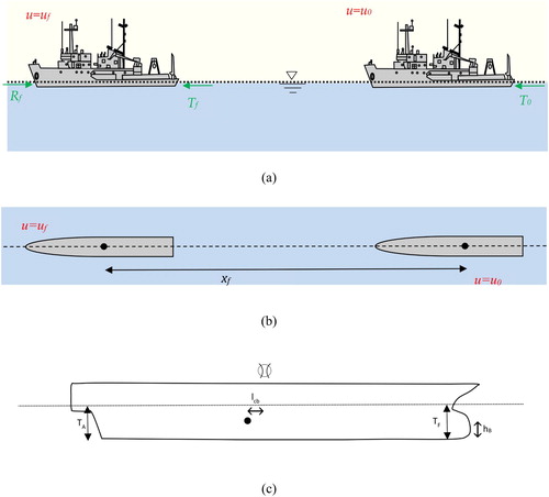
Ship acceleration, as mentioned earlier, is a type manoeuvring for ships, by which the vessel is accelerated forward from rest, and eventually reaches a steady motion (dynamic equilibrium) with a speed of u, depending on the power generated by the engine (Harvald 1983). The sketch of this motion is shown in Figure 1. Initially, the ship is floating on the water at rest and there is no wave, i.e. calm water condition. Then, the engine of the ship starts to work, and as a result, a torque is produced in by the engine. This torque then forces the propeller of the vessel to rotate. Consequently, a thrust force is caused by the propeller, drifting the ship forward. The rotation speed of the propeller increases up to the time a dynamic equilibrium between engine and propeller is established. In addition, ship accelerates forward up to the time summation of all forces acting on its surface, including resistance, thrust force, and added mass forces, becomes zero. Up to this time, ship would have had travelled a specific distance, shown by x_f. Note that in the current paper, the propulsion system (different from propeller) refers to engine and propeller, which together lead to propulsion of the ship.

Figure 1. A ship accelerating forward: (a) longitudinal view and (b) top view. The ship initially is at rest, and a thrust force, T₀, triggers the motion (right). Then, the speed of ship increases up to the time a dynamic equilibrium between all forces and moments is established (left). (c) shows some geometrical properties of the ship used for computation of the resistance.

Equation (1) governs on the motion of ship, which is established using the Newtons’ second law as (1) $\left(M+M_A\right)\frac{du}{dt}=R\left(t\right)+T_p\left(t\right)\left(1-t_p\right)$(1) where M is the ship mass, and M_A is the added mass of the ship in surge direction due to motion in the direction of surge. $R$ and $T_p$ denote resistance of the ship and thrust force of the propeller, respectively. It is assumed that no wind force acts on the body of the ship and no wave, either regular or irregular, and water current exits. Each of the forces acting on the body of the vessel varies in the time, depending on the ship speed, the rotational speed of propeller and the acceleration of the ship. A trust reduction coefficient, shown by $t_p$, is assumed to implement effects of the hull on the propeller. Equation (2) governs on the dynamic of the propeller of the ship, which is written as (2) $I\frac{dn}{dt}=Q_e-Q_i-Q_p.$(2)

In Equation (2), n is the rotational speed of the propeller. Q_e is the engine torque and Q_i is the torque loss. Q_pis the propeller torque, the value of which is sensitive to the different geometrical and physical characteristics of the propeller and advanced ratio of the propeller. Q_e depends on engine speed. In order to mathematically solve the above equations, it is necessary to determine forces acting on the rigid body (the ship) and the torque generated by the propeller from the beginning of the simulation until the final stage of the problem. Also, note that it is required to compute the added mass of the ship.

3. The resistance of the ship: Holtrop method

As mentioned in literature, different numerical methods can be used for computation of ship resistance, especially with the previous advances in CFD. It should be noted that CFD is known as a reliable hydrodynamic tool for the computation of ship resistance. But it is hard to use CFD for power prediction of ships in early-stage design when ship geometry has not been designed in detail, and the effects of many parameters are needed to be investigated in order to design the optimised ship. Among different proposed empirical methods for power prediction of ships, Holtrop method (Holtrop and Mennen 1978, 1982) has reached a high level, and its position was and still is secure among naval architects. Holtrop method has a good accuracy, and computes all resistance components of a ship operating in displacement regime. Equations of this method are developed based on experimental data, and can be linked to transient motion of the vessel, like acceleration or turning, easily. The method covers all types of hulls, and even provides the resistance of bulb and transom. Therefore, this method is used for the computation of the resistance of the ship in the current research. It is also worth mentioning that geometrical properties of the ship are illustrated in Figure 1(c).

It is assumed that ship resistance can be written as (3) $R_t=R_F\left(1+k_1\right)+R_W+R_B+R_{TR}+R_A.$(3) In Equation (3), R_t is total resistance of the ship. R_F, R_W, R_B, R_TR and R_A are, respectively frictional, wave-making, bulbus bow, transom and model correlation resistance terms (units of all is in N). Moreover, k₁ is the form factor of the ship (which does not have any dimension), that is used for the determination of the drag force caused by pressure loss. Frictional resistance ($R_F$ in N) can be computed by using the ITTC 57 as (4) $R_F=0.5{\rho }_w{u}^{2}S{C}_F,$(4) where ρ_wis the water density (Kg/m³), $S$ is the wetted surface of the ship (in m²) and C_F is the frictional resistance coefficient. Using the Holtrop method, the wetted surface of a displacement hull, denoted with $S$ (I m²), can be computed by (5) $\begin{array}{rl}S& =L\left(2T+B\right)\sqrt{C_M}\\ & \left(\begin{array}{c}0.453+0.4425C_B-0.2826C_M\\ -0.003467B/T+0.3696C_{WP}\end{array}\right)\\ & +2.38A_{BT}/C_B,\end{array}$(5) where L, T and B are the length, draft and beam of the ship, respectively. C_M is the midship section coefficient, and C_B is the block coefficient of the ship. Also, C_WP is the waterplane coefficient of the vessel. It should be noted that A_BT (in m²) in Equation (5) is the area of transverse section of the bulb. According to ITTC 57, the frictional resistance coefficient of a ship is computed by (6) $C_F=\frac{0.075}{{\left(\log {\mathcal{R}}_E-2\right)}^2},$(6) where ${\mathcal{R}}_E$is the Reynolds number, given by (7) ${\mathcal{R}}_E=\frac{uL}{\nu }.$(7)

In Equation (7), $\nu$ is the dynamic viscosity of the water and $u$ is the speed that can vary in time. It is important to note that additional frictional resistance, generated by the roughness of the hull, should also be considered. Therefore, Equation (4) is re-written as (8) $R_F=0.5{\rho }_W{u}^{2}S\left(C_F+\delta C_F\right),$(8) where $\delta CF$ is 0.0004, which refers to the roughness drag coefficient. 1 + k₁ (which does not have any dimensions), by which the drag caused by pressure loss is computed, is given by (9) $\begin{array}{rl}1+k_1& =c_{13}\{0.93+c_{12}{\left(B/L_R\right)}^{0.92497}\\ & {(0.95-C_p{)}^{-0.521448}-(1-C_p+0.0255l_{cb})}^{0.6909}\}.\end{array}$(9)

In Equation (9), L_R is length of run (in m), $C_P$ is the prismatic coefficient, l_cb is the longitudinal centre of buoyancy (in m). $c$₁₃ and $c$₁₂ are two non-dimensional coefficients. Length of run is computed by (10) $L_R/L=1-C_p+0.06\frac{C_p{l}_{cb}}{4C_p-1}.$(10)

c₁₂ is determined by using (11) $\left\{\begin{array}{ll}{c}_{12}={\left(\frac{T}{L}\right)}^{0.2228446}& \left(\frac{T}{L}\right)\text{ > 0}\text{.05 }\\ c_{12}=48.20{\left(\frac{T}{L}-0.02\right)}^{2.078}\\ +\text{ 0}\text{.479948}& \text{ 0}\text{.02 < }\left(\frac{T}{L}\right)\text{ < 0}\text{.05}\\ c_{12}=0.479948& \left(\frac{T}{L}\right)\text{ < 0}\text{.02 }\end{array}\right.$(11) Also, c₁₃ is found by (12) $c_{13}=1+0.003c_{stern},$(12) where c_stern is a coefficient that depends on the form of aft body section of the hull. If this section has V-shaped form, c_stern equals −10. If this section takes a U-shaped form, c_stern should be set to be 10. Otherwise, c_stern is set to be 0.

The wave-making resistance of the ship (in N) is estimated by empirical Equation (14), given by (13) $R_w=c_1{c}_2{c}_5\mathrm{\nabla }{\rho }_{w}gexp\left\{m_1\text{F}{\text{r}}^d+m_2\cos \left(\lambda \text{F}{\text{r}}^{-2}\right)\right\},$(13) where c₁, c₂, c₅, m_1, m₂ and $\lambda$ are non-dimensional coefficients. $\mathrm{\nabla }$ is the displacement volume of the ship. $g$ is the gravity acceleration (m/s²). $\text{Fr}$ stands for Froude Number of the vessel. c₁ is computed by (14) $c_1=2223105c_7^{3.78613}{\left(\frac{T}{B}\right)}^{1.07961}(90-i_e{)}^{-1.37565}.$(14)

In Equation (14), c₇ is a non-dimensional coefficient and $i_e$ is the entrance angle of the ship (in Deg). c₇ is determined by (15) $\left\{\begin{array}{ll}{c}_7=0.229577{\left(\frac{B}{L}\right)}^{0.3333}& \left(\frac{B}{L}\right)\text{ < 0}\text{.11}\\ c_7=\left(\frac{B}{L}\right)& \text{0}\text{.11 < }\left(\frac{B}{L}\right)\text{ < 0}\text{.25}\\ c_7=0.5-0.0625\left(\frac{L}{B}\right)& \left(\frac{B}{L}\right)\text{ < 0}\text{.25}\end{array}\right.$(15) On the other hand, i_e(in Deg.) is given by (16) $\begin{array}{rl}{i}_e& =1+89\left\{-{\left(\frac{L}{B}\right)}^{0.80856}{\left(1-c_{wp}\right)}^{0.30484}\right.\\ & {\left(1-C_P-0.0255l_{cb}\right)}^{0.6367}{\left(\frac{L_R}{B}\right)}^{0.34574}\\ & \left.{\left(100\frac{\mathrm{\nabla }}{L^3}\right)}^{0.16302}\right\}.\end{array}$(16) where $c_{wp}$ is the waterplane coefficient. c₂ is computed by (17) $c_2=exp\left(-1.89\sqrt{c_3}\right),$(17) where $c_3$ is a non-dimensional coefficient, computed as (18) $c_3=0.56\frac{A_{BT}^{1.5}}{BT\left(0.31\sqrt{A_{BT}}+T_F-h_B\right)}.$(18)

In Equation (18), h_B is the height of centre of bulb (in m) and T_F is fore draft. Finally, c₅ is predicted by (19) $c_5=1-\left(0.8\frac{A_T}{BT{C}_M}\right),$(19) where A_Tis the area of transom section (in m²) and C_M is the midship coefficient. Froude number of the ship is computed by using (20) $\text{Fr = }\frac{u}{\sqrt{gL}},$(20)

λ and m₁ are, respectively, computed by (21) $\left\{\begin{array}{ll}\lambda =1.446C_P-0.03\frac{L}{B}& \frac{L}{B}<12\\ \lambda =1.446C_P-0.36& \frac{L}{B}>12\end{array}\right.,$(21) and (22) $\begin{array}{rl}{m}_1& =0.0140407\frac{L}{T}-\left(1.75254\frac{{\mathrm{\nabla }}^{\frac{1}{3}}}{L}\right)\\ & -\left(4.79323\frac{B}{L}\right)-c_{16}.\end{array}$(22)

In Equation (22), c₁₆ is a non-dimensional coefficient, found by

(23) $\left\{\begin{array}{ll}{c}_{16}=8.07981C_P-\left(13.8673C_P^2\right)+6.984338C_P^3& C_P<0.80\\ c_{16}=1.73014-(0.7067C_P\text{)}& C_P>0.80\end{array}\right..$(23)

The value m₂ (which is used in Equation (13)) is computed by (24) $m_2=c_{15}{C}_P^{2}exp\left(-0.1\text{F}{\text{r}}^{-2}\right),$(24) where $c_{15}$ is a non-dimensional coefficient, computed by (25) $\left\{\begin{array}{ll}{c}_{15}=-1.69385& \frac{L^3}{\mathrm{\nabla }}<512\\ c_{15}=-169385+\frac{\left(\frac{L}{{\mathrm{\nabla }}^{1/3}}-8\right)}{2.36}& \text{ 512 < }\frac{L^3}{\mathrm{\nabla }}<1727\\ c_{15}=0& \frac{L^3}{\mathrm{\nabla }}>1727\end{array}\right.$(25)

The bulb resistance (in N) component is computed by (26) $R_B=0.11exp\left(-3K_B^{-2}\right)\text{F}{\text{r}}_i^3\frac{A_{BT}^{1.5}}{1+{\text{Fr}}_i^2}.$(26) where $K_B$ is a non-dimensional coefficient and Fr_i is the Froude Number of the bulb. $K_B$ is computed by (27) $K_B=0.56\frac{\sqrt{A_{BT}}}{T_F-1.5h_B}.$(27)

Froude number of bulb is given by (28) $\text{F}{\text{r}}_i=\frac{u}{\sqrt{g\left(T_F-h_B-0.25\sqrt{A_{BT}}\right)+0.15u^2}}.$(28)

Resistance of the transom (in N) is estimated by (29) $R_{TR}=0.5{\rho }_w{V}^2{A}_T{c}_6,$(29) where $A_T$ is the transom area (in m²), and c₆ is a non-dimensional coefficient. The value of c₆ is given by (30) $\left\{\begin{array}{ll}{c}_6=0.2\left(1-0.2\text{F}{\text{r}}_T\right)& \text{F}{\text{r}}_T<5\\ c_6=0& \text{F}{\text{r}}_T>5\end{array}\right..$(30)

In Equation (30), $\text{F}{\text{r}}_{\text{T}}$ is the Froude Number of transom, and can be computed by (31) $\text{F}{\text{r}}_T=\frac{u}{\sqrt{2g{A}_T/\left(B+B{C}_{WP}\right)}}.$(31)

Model correlation resistance (in N) is empirically approximated by (32) $R_A=0.5{\rho }_w{u}^{2}S{C}_A,$(32) where $C_A$ is the non-dimensional model correlation coefficient, and can be found by (33) $\begin{array}{rl}{C}_A& =0.006(L+100{)}^{-0.16}-0.00205\\ & +0.003\sqrt{\frac{L}{7.5}}{C}_B^4{c}_2\left(0.04-c_4\right).\end{array}$(33) $c_4$ is a non-dimensional coefficient, which depends on the draft of transom. $C_B$ is the bulk coefficient. Note that $c_2$ has been previously introduced. The value of $c_2$is calculated by (34) $\left\{\begin{array}{ll}{c}_4=\frac{T_F}{L}& \frac{T_F}{L}<0.04\\ c_4=0.04& \frac{T_F}{L}>0.04\end{array}\right..$(34)

4. Verification of the code in prediction of resistance

Holtrop method is a well-known method that its ability and accuracy is shown and accepted (Larsson and Raven 2010). However, in the current research, it is checked whether the developed code for this method is reliable or not. Therefore, the resistance of a displacement ship which has been previously measured by Olivieri et al. (2001) is predicted by the developed code, and then is compared against the published experimental data. Body lines of the investigated model, known as model INSEAN 2340, are shown in Figure 2. Principal characteristics of this hull are displayed in Table 1. This vessel has a U-shape form at its stern, and is only modelled in this Section. Results presented in Sections 8 and 9 correspond to another ship, which is later introduced.

Figure 2. Body line of the displacement hull, model INSEAN 2340, studied by Olivieri et al. (2003).

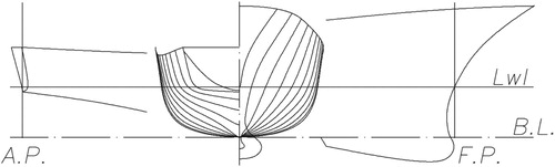
Table 1. Principal characteristics of the displacement hull, model INSEAN 2340, studied by Olivieri et al. (2001).

Parameter	Value
Scale factor	24.82
Length between perpendiculars (m)	5.72
Length at water level (m)	5.72
Beam (m)	0.76
Draft (m)	0.248
Trim angle (degrees)	0.00
Displacement (ton)	0.549
Volume (m^3)	0.549
Block coefficient	0.506
Prismatic coefficient	0.613
Midship section coefficient	0.825
Waterplane coefficient	0.778

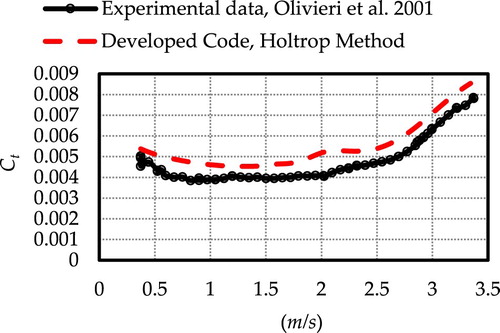
Predicted resistance and total resistance coefficient are shown in Figures 3 and 4. Total resistance coefficient is computed by (35) $C_t=\frac{R_t}{0.5{\rho }_w{u}^{2}S}.$(35) As can be seen in Figures 3 and 4, resistance and total resistance coefficient are well predicted. The trend of predicted resistance is similar to that of experimental data. Olivieri et al. 2001 reported that the resistance reaches 21.95 kg at the highest speed (corresponding to $u=3.34\text{m/s}$). The computed resistance at this speed is 23.32 kg at this speed, which is close to experimental data and supports the accuracy of the developed numerical code.

Figure 3. Comparison of predicted resistance and experimental data of Olivieri et al. 2001 for the model with body lines of Figure 2 and principal characteristics of Table 1.

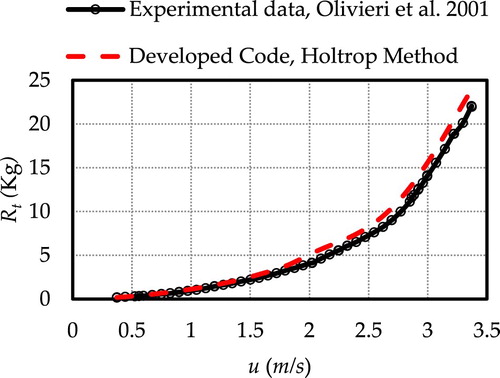
Figure 4. Comparison of predicted total resistance coefficient and experimental data of Olivieri et al. (2001) for the model with body lines of Figure 2 and principal characteristics of Table 1.

5. Performance of propeller: B-series

Thrust force and torque generated by the propeller, rotating with a speed of n, are required to be determined in order to solve equations of the motion in surge direction. Thrust coefficient is defined as (36) $K_T=\frac{T_p}{{\rho }_W{n}^2{D}^4},$(36) where D is the propeller diameter. Torque coefficient is defined as (37) $K_Q=\frac{Q_p}{{\rho }_w{n}^2{D}^5}.$(37)

Advanced ratio (which does not have any dimension) of the propeller is given by (38) $J=\frac{V_a}{nD}.$(38)

V_a is the advanced speed of the flow (in m/s) in the vicinity of the propeller given by (39) $V_a=u\left(1-\omega \right)$(39) where ω is the wake fraction coefficient (which does not have any dimension). Determination of the wake fraction is described in Section 5. Efficiency of the propeller is computed by (40) $\eta =\frac{K_t}{K_Q}\frac{J}{2\pi }$(40) In the current research, the B-Series propeller is assumed to be used for the generation of the thrust force of the ship. These special designs have been developed in the Netherlands Ship Model Basin, and are categorised as the fixed-pitch propellers. This series covers a wide range of standard shape of blades and pitch distributions. The open water tests of this series are available and regression equations, that can be used for computation of thrust force and torque, have been reported. This series has also been known as an interesting design that has been used in many academic researches.

Oosterveld and Ossannen (1975) conducted several open water tests on B-Series designs, and respectively formulated Equations (41) and (42) for computation of the thrust force coefficient and torque coefficient, (41) $\begin{array}{rl}{K}_T& =\sum _{N=1}^{39}{C}_N(J{)}^{S_N}{\left(\frac{P}{D}\right)}^{t_N}{\left(\frac{A_E}{A_o}\right)}^{u_N}(Z{)}^{v_N}\end{array}$(41) (42) $\begin{array}{rl}{K}_Q& =\sum _{N=1}^{47}{C}_N(J{)}^{S_N}{\left(\frac{P}{D}\right)}^{t_N}{\left(\frac{A_E}{A_o}\right)}^{u_N}(Z{)}^{v_N}\end{array}$(42)

In Equations (41) and (42), P is propeller pitch (in m), A_o is the propeller area (in m²), and A_E denotes expanded area (in m²). Moreover, Z refers to the number of blades. The other parameters, including C_N,, t_N, u_N and v_N are coefficients or orders used for prediction of the thrust force and torque. Note that, all these coefficients are found using regression studies. Their values are shown in Table 2. Sample of simulations for a B-Wageningen propeller with $A_E/A_O$ with Z = 3 and 4 at different $P/D$ is presented in Figure 5.

Figure 5. Sample of computed K_T and K_Q for B-Series propellers with A_E/A_o = 0.7: (a) Z = 3 and (b) Z = 4.

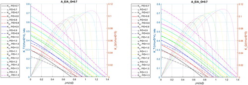
Table 2. Coefficients to be implemented in Equations (41) and (42).

KT						KQ
N	CN	SN	tN	uN	vN	N	CN	SN	tN	uN	vN
1	0.008805	0	0	0	0	1	0.0037937	0	0	0	0
2	−0.204554	1	0	0	0	2	0.0088652	2	0	0	0
3	0.166351	0	1	0	0	3	−0.032241	1	1	0	0
4	0.158114	0	2	0	0	4	0.0034478	0	2	0	0
5	−0.147581	2	0	1	0	5	−0.0408811	0	1	1	0
6	−0.481497	1	1	1	0	6	−0.108009	1	1	1	0
7	0.415437	0	2	1	0	7	−0.0885381	2	1	1	0
8	0.0144043	0	0	0	1	8	0.188561	0	2	1	0
9	−0.0530054	2	0	0	1	9	−0.0037087	1	0	0	1
10	0.0143481	0	1	0	1	10	0.005137	0	1	0	1
11	0.0606826	1	1	0	1	11	0.0209449	1	1	0	1
12	−0.0125894	0	0	1	0	12	0.0047432	2	1	0	1
13	0.0109689	1	0	1	0	13	−0.0072341	2	0	1	1
14	−0.133698	0	3	0	0	14	0.0043839	1	1	1	1
15	0.0063841	0	6	0	0	15	−0.0269403	0	2	1	1
16	−0.0013272	2	6	0	0	16	0.0558082	3	0	1	0
17	0.168496	3	0	1	0	17	0.0161886	0	3	1	0
18	−0.0507214	0	0	2	0	18	0.0031809	1	3	1	0
19	0.0854559	2	0	2	0	19	0.015896	0	0	2	0
20	−0.0504475	3	0	2	0	20	0.0471729	1	0	2	0
21	0.010465	1	6	2	0	21	0.0196283	3	0	2	0
22	−0.0064827	2	6	2	0	22	−0.0502782	0	1	2	0
23	−0.0084173	0	3	0	1	23	−0.030055	3	1	2	0
24	0.0168424	1	3	0	1	24	0.0417122	2	2	2	0
25	−0.001023	3	3	0	1	25	−0.0397722	0	3	2	0
26	−0.0317791	0	3	1	1	26	−0.0035002	0	6	2	0
27	0.018604	1	0	2	1	27	−0.0106854	3	0	0	1
28	−0.004108	0	2	2	1	28	0.001109	3	3	0	1
29	−0.0006068	0	0	0	2	29	−0.0003139	0	6	0	1
30	−0.0049819	1	0	0	2	30	0.0035985	3	0	1	1
31	0.0025983	2	0	0	2	31	−0.0014212	0	6	1	1
32	−0.0005605	3	0	0	2	32	−0.0038364	1	0	2	1
33	−0.0016365	1	2	0	2	33	0.0126803	0	2	2	1
34	−0.0003288	1	6	0	2	34	−0.0031828	2	3	2	1
35	0.0001165	2	6	0	2	35	0.0033427	0	6	2	1
36	0.0006909	0	0	1	2	36	−0.0018349	1	1	0	2
37	0.0042175	0	3	1	2	37	0.0001125	3	2	0	2
38	5.652E−05	3	6	1	2	38	−2.972E−05	3	6	0	2
39	−0.0014656	0	3	2	2	39	0.0002696	1	0	1	2
						40	0.0008327	2	0	1	2
						41	0.0015533	0	2	1	2
						42	0.0003027	0	6	1	2
						43	−0.0001843	0	0	2	2
						44	−0.0004254	0	3	2	2
						45	8.692E−05	3	3	2	2
						46	−0.0004659	0	6	2	2
						47	5.542E−05	1	6	2	2

6. Engine modelling

In order to simulate the performance of engine, a previous mathematical model proposed by Altosole and Figari (2011) has been utilised. Based on their proposed equation for brake power of the engine (in W), it can be written that (43) $\begin{array}{rl}{P}_B& ={\left(\frac{m_{fd}}{m_f}\right)}^{3/2}\left(a{\left(\frac{m_{fd}}{m_f}\right)}^{3/2}{n}_e^3\right.\\ & \left.+b{\left(\frac{m_{fd}}{m_f}\right)}^{3/2}{n}_e^2+c{\left(\frac{m_{fd}}{m_f}\right)}^{3/2}{n}_e\right)\end{array}$(43) where m_f is the fuel flow rate and n_e is the engine speed. a, b and c are three coefficients used for computation of the brake power. In addition, the torque (in N-m) generated by the engine can be computed by using (44) $\begin{array}{rl}{Q}_e& =\frac{1}{2\pi }{\left(\frac{m_{fd}}{m_f}\right)}^{1.35}\left(a{\left(\frac{m_{fd}}{m_f}\right)}^{1.35}{n}_e^3\right.\\ & \left.+b{\left(\frac{m_{fd}}{m_f}\right)}^{0.9}{n}_e^2+c{\left(\frac{m_{fd}}{m_f}\right)}^{0.45}{n}_e\right).\end{array}$(44)

It is important to comment that in order to find a, b and c, it is necessary to use the performance diagrams of the engines, which are published by industrial companies. In order to find these three parameters, the least square method (Hamming 1962) has been used in the current study.

7. Hull-propeller interactions

As stated earlier, modelling the interaction between hull and propeller leads to two different points that needs consideration of the drag reduction and wake fraction. To find these two parameters, previous empirical equations of Holtrop are utilised. These equations have been found by using statistical data and finalised by Holtrop. Wake fraction can be determined by using Equation (45) as (45) $\begin{array}{rl}\omega & =c_9{C}_V\frac{L}{T_A}\left(0.0661875+1.21756c_{11}\frac{C_V}{\left(1-C_{p1}\right)}\right)\\ & +0.24558\sqrt{\frac{B}{\left(1-C_{p1}\right)}}-\left(\frac{0.09726}{0.95-C_P}\right)+\frac{0.11434}{0.95-C_P}.\end{array}$(45) where $c_9$ and c₁₁ are non-dimensional coefficient. $C_V$ is a resistance coefficient embracing effects of viscosity, form drag and model correlation. $C_{p1}$ is the effective prismatic coefficient. $c_9$ is computed by (46) $\left\{\begin{array}{ll}{c}_9=c_8& c_8<28\\ c_9=32-\left(\frac{16}{c_8-24}\right)& c_8>28\end{array}\right.$(46) c₈ in the Equation (46) is a non-dimensional coefficient, which is estimated by using (47) $\left\{\begin{array}{ll}{c}_8=\frac{BS}{LD{T}_A}& \frac{B}{T_A}<5\\ c_8=S\frac{7\frac{B}{T_A}-25}{LD\left(\frac{B}{T_A}-3\right)}& \frac{B}{T_A}>5\end{array}\right..$(47) c₁₁ is determined by the empirical equation of (48) $\left\{\begin{array}{ll}{c}_{11}=\frac{T_A}{D}& \frac{T_A}{D}<2\\ c_{11}=0.0833333{\left(\frac{T_A}{D}\right)}^3\text{ + 1}\text{.333}& \frac{T_A}{D}>2\end{array}\right..$(48)

C_Vin Equation (45) is estimated by using (49) $C_V=C_F\left(1+k_1\right)+C_A,$(49) and C_p1is computed by (50) $C_{p1}=1.45C_p-0.315-0.0225l_{cb}.$(50)

The trust reduction coefficient is found by using Equation (51) as (51) $\begin{array}{rl}{t}_p& =0.001979\frac{L}{B-B{C}_{P1}}+1.0585c_{10}-0.00524\\ & -0.1418\frac{D^2}{BT}+0.0015C_{Stern},\end{array}$(51) where $c_{10}$ is a non-dimensional coefficient, and its value is estimated by (52) $\left\{\begin{array}{ll}{c}_{10}=\frac{B}{L}& \frac{L}{B}>5.2\\ c_{10}=0.25-(\frac{0.003328402}{\frac{B}{L}-0.134615385}\text{)}& \frac{L}{B}<5.2\end{array}\right..$(52)

8. Simulation of the problem

As stated earlier, the problem contains ordinary differential equations. In order to solve these equations, numerical methods should be used. However, before solving these equations, it is necessary to compute the added mass of the ship. In order to compute the added mass of the ship, an empirical equation is used. This equation has been previously used for ships and can be found in a report published by Toxopeus (1996). Added mass is computed by Equation (53) as (53) $M_A=\frac{\pi {\rho }_W{T}^{2}B}{2}{C}_M.$(53) Dynamic of the ship-propeller-engine obey Equation (54) as (54) $\begin{array}{rl}& \left(M+M_A\right)\frac{\text{d}u}{\text{d}t}=R+T_p\left(1-t_p\right)\\ & I\frac{\text{d}n}{\text{d}t}=Q_e-Q_i-Q_p\\ & \frac{\text{d}{m}_f}{\text{d}t}=f\left(\dot{n_e},n_e\right)=-c_p\dot{n_e}+c_I\left[n_c-n_e\right].\end{array}$(54) where $n_c$ is the command shaft speed. $c_p$ and $c_I$ are, respectively, proportional gain of the control equation of the shaftline and integral gain of the control equation of the shaftline.

As it can be seen Equation (54), another sub-equation is added to the system. This very last sub-equation represents the variation of the fuel mass flow rate as a function of shaft rotational speed rate. In the current paper, it is assumed that, the fuel mass flow rate is a function of engine speed as suggested by Altosole and Figari (2011). Also, the engine is assumed to be diesel with two-storkes. More technical information about the dynamic of engine can be found in Altosole and Figari (2011).

To numerically solve the problem in the time domain, a 4th Order Runge–Kutta Method has been used (see detail of the method in Hamming 1962). Therefore, each parameter is found by using (55) $y_{i+1}=y_i+\frac{\mathrm{\Delta }t}{6}\left(K_1+2K_2+2K_3+K_4\right).$(55) where (56) $\begin{array}{l}{K}_1=f\left(y_i,t_i\right)\\ K_2=f\left(y_i+K_1\frac{\mathrm{\Delta }t}{2},t_i+\frac{\mathrm{\Delta }t}{2}\right)\\ K_3=f\left(y_i+K_2\frac{\mathrm{\Delta }t}{2},t_i+\frac{\mathrm{\Delta }t}{2}\right)\\ K_4=f\left(y_i+K_3\mathrm{\Delta }t,t_i+\mathrm{\Delta }t\right).\end{array}$(56)

Simulations for a ship with principal characteristics of Table 3 are performed. Note that, this ship is different from the model introduced in Section 4. The ship, with information shown in Table 3, is the one that is model in Hotrop (1984a) and has a stern with a U-form shape. It should be noted that two different pitch values are considered to show that different inputs can lead to different acceleration results.

Table 3. Principal characteristics of the investigated ship.

Parameter	Value
Length on water line (m)	205
Length between perpendiculars (m)	200
Beam (m)	32
Draft (m)	10
Draft at F.P (m)	10
Draft at A.P (m)	10
Trim angle (degrees)	0.00
Displacement (ton)	38430
Volume (m^3)	37500
Block coefficient	0.571
Prismatic coefficient	0.583
Midship section coefficient	0.98
Waterplane coefficient	0.75
Propeller Diameter (m)	8
Number of blades	3
P/D	0.9-1
AE/Ao	0.6

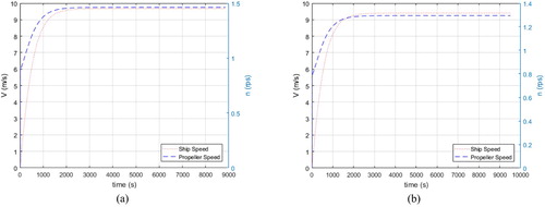
Predicted resistance for this ship is shown in Figure 6. Simulations of acceleration of the considered ship for the two different pitches are displayed in Figure 7. As obvious in this figure, the results of the developed method and provided numerical code behave as expected. It means that propeller and ship, finally reach a steady state. Propeller reaches its final speed earlier in comparison with ship. The interesting point in this figure is about final speed and the time needed for the vessel to reach it. The maximum speed of the ship is larger for the P/D = 0.9 in comparison with that of P/D = 1.0. With the former pitch, ship reaches a final speed of 9.8 m/s, while with the latter the speed of the ship converges to 9.2 m/s. It should be mentioned that, in the case the ship reaches a larger speed, the time needed to reach this speed is greater. Again, it should be noted that the results in this Figure are just examples to show the abilities of the developed method.

Figure 6. Computed resistance for the investigated displacement ship.

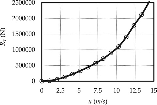
Figure 7. Simulation of acceleration of investigated ship: (a) P/D = 0.9 and (b) P/D = 1.0.

9. Application of the method in design: optimisation of the propulsion system

The proposed code and method are used to design an optimise propeller for the ship with the information given in Table 3. To this end, a multi-objective design is performed in order to optimise three different parameters. It is aimed to minimise the time needed to reach the final speed, maximise the final speed of the vessel, push the vessel forward with the most efficient propeller. Note that this optimisation is only performed to show that the method can be linked to optimisation libraries and no design aim is followed in this section. That is, it is attempted to demonstrated that the code is flexible enough to be used for even optimisation aims. Upper and lower bands of the propeller are shown in Table 4.

Table 4. Upper and lower bands of the propeller.

Targeted parameter	Upper band	Lower band
Propeller Diameter (m)	6	10
AE/Ao	0.3	1.1
P/D	0.6	2.0
Number of blades	3	6

In addition to previously explained parameters, cavitation constraint, taken from Keller (1966), is set to be satisfied. Equation (57) gives the cavitation constraint as (57) ${\left(\frac{A_E}{A_O}\right)}_{min}=\frac{\left(1.3+0.3Z\right)T_p}{\left(p_s-p_v\right)}+0.2$(57) where $p_s$ is the vapour pressure and $p_s$ is the static pressure behind the axis of the propeller. Also, a strength constraint is defined as (58) $\begin{array}{rl}& {\left(\frac{t_{min}}{D}\right)}_{0.7R}\\ & =0.0028+0.21\sqrt[3]{\frac{3183.87-1508.15\left(P/D\right)P_s}{1266652.04n{D}^3\left(S_c+20.9D^2{n}^2\right)}}.\end{array}$(58) where S_c is the maximum allowable stress (in Pa) and P_S is the shaft power. This constraint is also defined to make sure that the propeller has enough strength. Maximum blade thickness values of B-series at different conditions are reported in Table 5.

Table 5. Upper and lower bands of the propeller.

	Maximum blade thickness (% of D)
r/R	Z = 3	Z = 4	Z = 5
0.2	4.06	3.66	3.26
0.3	3.59	3.24	2.89
0.4	3.12	2.82	2.52
0.5	2.65	2.40	2.15
0.6	2.18	1.98	1.78
0.7	1.71	1.56	1.41
0.8	1.24	1.14	1.04
0.9	0.77	0.72	0.67
1.0	0.30	0.30	0.30

Optimisation is performed by using genetic algorithm and non-dominated sorting genetic algorithm-II (NSGA-II) method. Firstly initial values for parameters are defined. Then, simulations of the ship motion in surge direction are performed by using initial values. Then, iterations are performed in order to find the optimised values. Within each iteration, responses corresponding to each propeller are determined and compared with previous data. Then, cross over and mutations techniques are carried out in order to generate new offspring. In the next step, parent and child population will be combined. Afterward, the parents will be replaced by the best combined population that was found in the previous step. These iterations are continued up to the occurs and objectives converge.

Optimisation has been performed and optimised values are found and shown in Table 6. Acceleration behaviours of the investigated ship (with information shown in Table 3) under both conditions, before optimisation and after optimisation, are simulated and displayed in Figure 8. As apparent, when the optimised propeller is used to push the vessel forward, the final speed of the vessel exceeds 12 m/s. Also, the time at which the speed plot starts to converge is smaller. Variation in the rotational speed of the propeller of the vessel during the acceleration with and without the optimised propeller is illustrated in Figure 9. According to the curves of this figure, one may be seen is that, under the optimised condition, the speed of the propeller increases. However, it can be seen that for both cases, the steady state of the propeller behaviour starts at approximately similar times.

Figure 8. Comparison of the acceleration performance of the ship with and without optimised propeller.

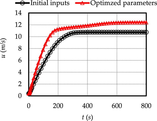
Figure 9. Comparison of the rotation speed of the ship with and without optimised propeller.

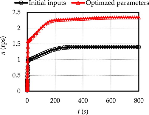
Table 6. Initial values and optimised values of parameters.

Targeted parameter	Initial value	Optimised value
Propeller Diameter (m)	8	8.25
AE/Ao	0.8	0.77
P/D	0.9	1.89
Number of blades	3	4

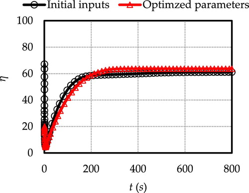
Figure 10 reports the time history of the propeller efficiency of both cases, including initial and optimised parameters. The curves in this figure suggest that when the optimised propeller is used, the efficiency of the propeller increases from 59% to 63% in the steady-state condition. However, before steady-state condition, propeller efficiency of the non-optimised propeller is lower.

Figure 10. Comparison of the propeller efficiency of the ship with and without optimised propeller.

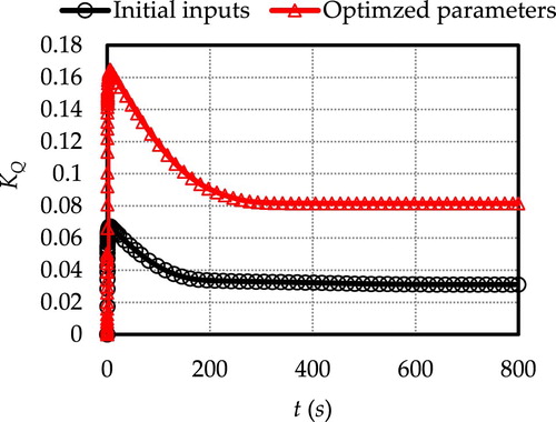
Time-histories of thrust force and torque coefficients of the propeller of the before and after optimisation are shown in Figures 11 and 12, respectively. One can be seen in this figure is that under the force of the optimised propeller, thrust coefficient and torque coefficient become larger. The interesting point is that, in steady operation, thrust force is increased up to 92%, while torque moment is increased up to 260%. Overall, it can be seen that the model properly work, and the optimised values lead to better performance. Also, note that the cavitation limit is also satisfied. If it is assumed that the hub propeller has a depth of 6 m, the static pressure will be 1.61 × 105 pa. The vapour pressure of the water for a temperature of 20 degrees is set to be 0.07 × 105 pa. If the mentioned values are substituted in Equation (58), the minimum value of A_E/A_O in is found to be 0.64, which is smaller than the optimised value (assume that t_p = 0.17 and Resistance of the ship at the final speed is 1.63 × 10⁶ N).

Figure 11. Comparison of thrust force coefficient of the ship with and without optimised propeller.

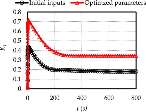
Figure 12. Comparison of torque coefficient of the ship with and without optimised propeller.

10. Concluding remarks

In this paper, a mathematical model was developed for simulation of the acceleration motion of displacement ships. This model uses the previous empirical methods for the computation of ship resistance and the performance of the propeller. Dynamic behaviour of the engine is predicted by using previous models. Added mass of the ship is estimated by using an empirical equation.

Accuracy of the developed code for resistance prediction of ships was evaluated by comparing the obtained results against published experimental data. Examples of the outcome of the simulations were presented for two different propellers, showing that a different design can affect both final speed and the convergence time. Then, the method was combined with genetic algorithm in order to show how the model can be used for different aims, such as optimisation. Initial inputs were implemented and then the optimised parameters were found. It was shown that, as the optimised parameters were used, ship reaches higher speeds. Optimisation results showed that the optimised propeller has higher rotational speed and the thrust force and torque coefficients, corresponding to the optimised propeller, are larger than the values corresponding to the initial propeller.

The current work provides early but useful simulations for the acceleration of ships. It can provide an understanding of the physics of the problem when the dynamic of the propulsion system is coupled with transient surge motion. But, in future, the method is needed to be corrected and more different physical factors, and more accurate models for the engine are needed to be considered, which lead to more reliable simulations. The studies carried out by Altosole et al. 2019 and Altosole et al. 2020 can be helpful for this aim.

Disclosure statement

No potential conflict of interest was reported by the author(s).

References

- Altosole M, Benvenuto G, Campora U, Silvestro F, Terlizzi G. 2018. Efficiency improvement of a natural gas marine engine using a hybrid turbocharger. Energies. 11(8):1924.
- Altosole M, Benvenuto G, Figari M, Coampora U. 2008. Real-time simulation of a COGAG naval ship propulsion system. In Proceedings of Maritime Industry, Ocean Engineering and Coastal Resources – Proceedings of the 12th International Congress of the International Maritime Association of the Mediterranean, IMAM 2007.
- Altosole M, Benvenuto G, Zaccone R, Campora U. 2020. Comparison of saturated and superheated steam plants for waste-heat recovery of dual-fuel marine engines. J Mar Sci Eng. 7(5):138.
- Altosole M, Campora U, Figari M, Laviola M, Martelli M. 2019. A diesel engine modelling approach for ship propulsion real-time simulators. J Mar Sci Eng. 7(5):138.
- Altosole M, Figari M. 2011. Effective simple methods for numerical modelling of marine engines in ship propulsion control systems design. J Naval Archit Mar Eng. 8(2):129–147.
- Altosole M, Figari M, Bagnasco A, Maffioleti L. 2007. Design and test of the propulsion control of the Aircraft Carrier ‘cavour’ using real-time hardware in the loop simulation, In Proceedings of the SISO European Simulation Interoperability Workshop 2007.
- Dagan G. 1972. Small Froude number paradoxes and wave resistance at low speeds. Tech. Rep. 7103-4, Hydronautics Inc., Laurel, MD, USA.
- Dashtimanesh A, Tavakoli S, Kohansal A, Khosravani R, Ghassemzadeh A. 2020. Numerical study on a heeled one-stepped boat moving forward in planing regime. Appl Ocean Res. 96:102057.
- Esfandiari A, Tavakoli S, Dashtimanesh A. 2019. Comparison between the dynamic behavior of the non-stepped and double-stepped planing hulls in rough water: a numerical study. J Ship Prod Des. 36(1):1–15.
- Ferrando M, Scamardella A, Bose N, Liu P, Veitch B. 2002. Performance of a family of surface piercing propellers. Trans R. Inst Naval Architects Part A: Int J Maritime Eng. 144:63–77.
- Figari M, Altosole M. 2007. Dynamic behaviour and stability of marine propulsion systems. Proc Inst Mech Eng Part M: J Eng Maritime Environ. 221:187–202.
- Froude RE. 1881. On the leading phenomena of the wave-making resistance of ships. Trans Inst Naval Architects. 22:220–245.
- Froude RE. 1888. On the ‘constant’ system of notation of results of experiments on models used at the admiralty experiments works. Trans Inst Naval Architects. 29:304–318.
- Geertsma RD, Negenborn RR, Visser K, Hopman JJ. 2016. Torque control for diesel mechanical and hybrid propulsion for naval vessels. Proceedings of the 13th INEC, Bristol, UK.
- Geertsma RD, Negenborn RR, Visser K, Hopman JJ. 2017. Pitch control for ships with diesel mechanical and hybrid propulsion: modelling, validation and performance quantification. Appl Energy. 226:1609–1631.
- Ghadimi P, Tavakoli S, Dashtimanesh A, Pirooz A. 2014. Developing a computer program for detailed study of planing hull’s spray based on Morabito’s approach. J Mar Sci Appl. 13:402–415.
- Ghadimi P, Tavakoli S, Dashtimanesh A, Zamanian R. 2017. Steady performance prediction of a heeled planning craft in calm water using asymmetric 2D+T model. P I Mech Eng M-J Eng. 231(1):1–24.
- Harvald SA. 1983. Resistance and propulsion of ships, Volume 12 of Ocean engineering, Wiley.
- Hemmining. 1962. Numerical Methods for Scientists and Engineers.
- Holtrop J. 1984a. A statistical re-analysis of resistance and propulsion data. Int Shipbuilding Prog. 31:272–276.
- Holtrop J. 1984b. A statistical resistance prediction method with a speed dependent form factor. In Scientific and Methodological Seminar on Ship Hydrodynamics (SMSSH ‘84), Varna, Bulgaria.
- Holtrop J, Mennen G. 1978. A statistical power prediction method. Int Shipbuilding Prog. 25:253–256.
- Holtrop J, Mennen G. 1982. An approximate power prediction method. Int Shipbuilding Prog. 29:166–170.
- Huang L, Li M, Romu T, Dolatshah A, Thomas G. 2020. Simulation of a ship operating in an open-water ice channel, ships and offshore structures. doi: 10.1080/17445302.2020.1729595
- Huang L, Ren K, Li M, Tukovic Z, Cardiff P, Thomas G. 2019. Fluid-structure interaction of a large ice sheet in waves. Ocean Eng. 181:102–111.
- Huang L, Thomas G. 2019. Simulation of wave interaction with a circular ice floe. J Offshore Mech Arct Eng. 141(4):1–9.
- Hughes G. 1954. Friction and form resistance in turbulent flow, and a proposed formulation for use in model and ship correlation. Trans Inst Naval Architects. 96:314–376.
- IMO. 2015. Third IMO greenhouse gas study 2014, exec, summary and final report, Technical Report, IMO, London, UK.
- ITTC. 1957. 8th International Towing Tank Conference, Madrid Spain. ITTC. Available at www.ittc.info.
- ITTC. 1978. Proceedings of the 15th ITTC, The Hague, The Netherlands. Netherlands Ship Model Basin.
- Javanmardi N, Ghadimi P, Tavakoli S. 2018. Probing into the effects of cavitation on hydrodynamic characteristics of surface piercing propellers through numerical modeling of oblique water entry of a thin wedge. Brodogradnja: Teorija i praksa brodogradnje i pomorske tehnike. 69(1):151–168.
- Keller J. 1966. Enige Aspecten Bij Het Antwerpen Van Scheepsschroeven. Schpen Werf 24.
- Larsson L, Raven HC. 2010. Ship resistance and flow: The Principles of Naval Architecture Series, SNAME, Jersey City, NJ, US.
- Larsson L, Stern F, Bertram V. 2003. Benchmarking of computational fluid dynamics for ship flows: The Gothenburg 2000 workshop. Journal of Ship Research. 47(1):63–81.
- Niazmand Bilandi R, Dashtimanesh A, Tavakoli S. 2020. Hydrodynamic study of heeled double-stepped planing hulls using CFD and 2D+ T method. Ocean Eng. 196:106813.
- Odetti M, Altosole M, Bruzzone G, Caccia M, Viviani M. 2019. Design and construction of a modular pump-jet thruster for autonomous surface vehicle operations in extremely shallow water. J Mar Sci Eng. 7(7):222.
- Ogilvie TF. 1968. Wave resistance: The low-speed limit. Report No. 002. Ann Arbor, MI: Univ. Michigan, Dept. Nav. Arch. Mar. Eng. (MARIN): Wageningen, Netherlands.
- Olivieri A, Pistani F, Avanzini A, Stern F, Penna R. 2001. Towing tank experiments of resistance, sinkage and trim, boundary layer, wake, and free surface flow around a naval combatant insean 2340 model, IIHR Technical Report No. 421.
- Olivieri A, Pistani F, De Mascio A. 2003. Breaking wave at the bow of a fast displacement ship model. J Mar Sci Technol. 8(2):68–75.
- Oosterveld MWC. 1970. Wake adapted ducted propellers, NSMB Wageningen Publication No. 345.
- Oosterveld MWC. 1973. Ducted propeller characteristics. RINA Symposium on Ducted Propellers.
- Oosterveld MWC, Ossannen PV. 1975. Further computer-analyzed data of Wageningen B-screw series. ISP, 22(251):3–14.
- Reynolds O. 1883. An experimental investigation of the circumstances which determine whether the motion of water shall be direct or sinuous, and the law of resistance in parallel channels. Philos Trans R. Soc. 174:935–998.
- Roskilly AP, Palacin R, Yan J. 2015. Novel technologies and strategies for clean transport systems. Appl Energy. 157:533–536.
- Rotte GM. 2015. Analysis of a hybrid RaNS-BEM method for predicting ship power, M.Sc thesis, TU Delft, Delft, Netherlands.
- Tavakoli S, Dashtimanesh A. 2019. A six-DOF theoretical model for steady turning maneuver of a planing hull. Ocean Eng. 189:106328.
- Tavakoli S, Najafi S, Amini E, Dashtimanesh A. 2018. Performance of high-speed planing hulls accelerating from rest under the action of a surface piercing propeller and an outboard engine. Appl Ocean Res. 77:45–60.
- Toxopeus S. 1996. A time domain simulation program for maneuvering of planing ships. Delft: Delft University of Technology.
- van Oortmerssen G. 1971. Power prediction method and its application to small ships, Netherlands Ship Model Basin. Wageningen, Netherland: Wageningen.
- Zaccone M, Ottaviani E, Figari M, Altosole M. 2018. Ship voyage optimization for safe and energy-efficient navigation: a dynamic programming approach. Ocean Eng. 153:215–224.