Impact of DHM resolution on gravity anomalies and geoid undulations: case study for Egypt

ABSTRACT

This study aims to estimate the effect of the resolution of the available Digital Height Models (DHMs) on the reduced gravity anomalies and the final computed gravimetric geoid. The region of Egypt is taken to be a prototype test. Different available DHMs are used in this study. The window technique has been used for gravity reduction (Abd-Elmotaal and Kühtreiber 2003). The reduced gravity anomalies are used to compute geoid undulations in each test case employing the 1D-FFT technique. The comparison among the results has been carried out at two levels: the reduced gravity anomalies and the discrepancy in geoid undulations. The results show that using fine DHM with a resolution of $3^{\prime \prime }$ x $3^{\prime \prime }$ or using fine DHM with a resolution of $1^{\prime \prime }$ x $1^{\prime \prime }$, with a coarse DHM with a resolution of ${30}^{\prime \prime }$ x ${30}^{{ }^{\prime \prime }},$ gives approximately the same results according to the range and the standard deviation. On the other hand, applying $3^{\prime \prime }$ x $3^{\prime \prime }$ DHM resolution saves about 80% of the central processing unit (CPU) time necessary for the reduction step. The results show that the difference between the indirect effect in the case of fine DHM $1^{\prime \prime }$ x $1^{\prime \prime }$ and the case of fine DHM with a resolution of $3^{\prime \prime }$x $3{ }^{\mathrm{\prime \prime }}$ is very small (about 1 cm). This means that going to $1^{\prime \prime }$ x $1^{\prime \prime }$ DHM is not needed for the test region as $3^{\prime \prime }$ x $3{ }^{\mathrm{\prime \prime }}$ can save time and effort and give approximately the same results in both gravity reduction and geoid computation. Finally, it can be concluded that using fine DHM with a resolution of $1^{\prime \prime }$ x $1^{\prime \prime }$ and coarse DHM with a resolution of ${30}^{\prime \prime }$ x ${30}^{\prime \prime }$ are adequate for determining the gravity anomalies and gravimetric geoid for Egypt.The geoid undulation differences between the GPS/levelling points of HARN and our developed geoid provide improvements by about 10 cm concerning the geoid computed from EGY-HGM2016 model . These improvements are considered to be important when we are seeking about 1 cm geoid.

KEYWORDS:

• Egypt
• digital height model
• window technique
• gravity reduction
• geoid computation

1. Introduction

Because it is essential to utilise the geoid as a reference surface when estimating a point’s elevation its precise estimation is crucial for surveying and mapping. Tscherning and Forsberg (1986), Tziavos (1987), Vaniček and Kleusberg (1987), Denker (1991), Ayhan (1993), Denker et al. (1994), Milbert (1993), Vaniček et al. (1995), Sideris and She (1995), Denker and Torge (1993), and Denker et al. (1995) all reported significant improvements in the geoid determination. Geoid heights are now the standard information used in geophysical interpretations. The following topics are covered by the geophysical applications of the geoid: (1) the anomalies in the density of the upper crust (Fotiou et al. 1988); (2) the structure of the deep Earth mass anomaly (Hager 1984; Bowin et al. 1986, 1994); (3) the strain and stress field (Livieratos 1987; Dermanis et al. 1992; Livieratos et al. 1994); (4) tectonic forces (Pick et al. 1994), (5) lithosphere structure of the oceans (Forsyth 1985; Sandwell and Mckenize 1989; Wunsch and Stammer 1993; Cazenave et al. 1994), (6) Earth’s rotation (Chao et al. 1994), (7) geophysical prospecting (Hayling et al. 1994), and rotation of the Earth.

A digital Height Model (DHM) is a computer depiction of the Earth’s surface that serves as a baseline dataset from which topographic characteristics may be digitally created. For instance, DHMs are employed in geoid modelling, geo-morphological simulation and classification, and hydrological run-off modelling to calculate terrain correction and downward continuation (DWC) corrections. Although a DHM is merely an elevation surface model, it might contain mistakes like other models (e. g. Hilton et al. 2003). It is crucial to assess the correctness of the DEM in the interest region before utilising it, just like with any other source of data used in geoid determination (such as gravitational models and gravity information).

The derivation of geoids, gravity interpretation, and gravity inversion are only a few geodetic and geophysical applications that are influenced by accurate and effective terrain modelling (Hammer 1939; LaFehr 1991; Martinec et al. 1996; Leaman 1998). Both the forward and inverse methods of gravity field interpretation utilise geometric modelling of the mass distribution between a topographical relief and a reference surface in the Earth’s interior or of a single buried mass anomaly, as well as the numerical computation of the associated gravitational signal at arbitrary space points (Blakely 1996; Nowell 1999; Li and Goetze 2001).

One of the key problems in local and regional gravity field studies is how to adequately and effectively describe the corresponding mass distributions given the structure of the different layers of the Earth’s interior, including the crust-mantle boundary (Bassin et al. 2000). Additionally, more precise modelling of the terrain masses is possible thanks to the ongoing improvement in resolution of the currently available crustal and terrain information, mostly but not only as a result of the use of satellite observations.

To calculate the gravitational potential and its first-order derivatives (gravitational vector) caused by the provided mass distribution, two key facts are needed including, the geometry of the source and knowledge of the associated mass density distribution. According to Huang et al. (2001), the mean mass density is utilised herein to explain and depict the actual mass density distribution of the topographical masses rather than mass density distribution, which isn’t addressed in the current contribution.

There are many factors affecting the precise determination of the gravimetric geoid. These are the coverage of the gravity data information, the precision of gravity data, the density of the topographic masses, the precision of the digital height model, and the resolution of DHM (El-Ashquer et al. 2016; El Shouny et al. 2018; Elwan et al. 2021). In this investigation, the resolution of DHMs has been studied in detail for a case study in Egypt.

From the above paragraph, it can be seen that the DHM is important for destemming the gravimetric geoid for Egypt. As it plays an important role in computing the terrain corrections and the indirect effects. These parameters (terrain correction and indirect effects) are computed using two Digital Height Models: the Fine Digital Height model in the inner zone and the coarse Digital Height Model in the outer zone. The precision of the final Gravimetric geoid depends on the resolutions of the two DHMs. On the other hand, the Central Processing Unit (CPU) depends on the resolutions of the two DHMs. Therefore, this paper aims to find the best resolutions for the two DHMs that give minimum CPU time and the best accuracy.

2. Used data

2.1. Gravity data

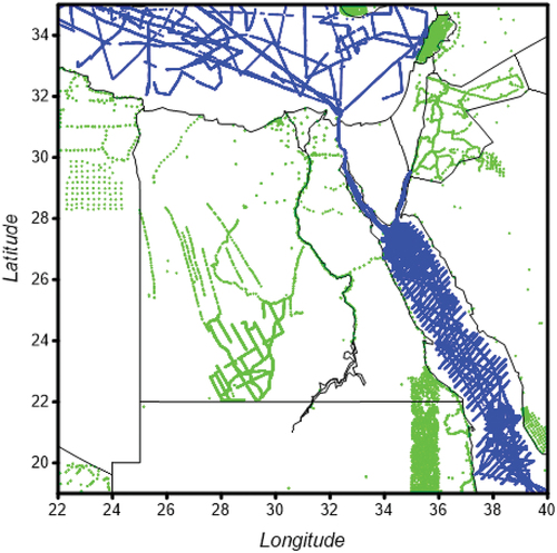
The gravity anomalies information presented in Figure 1 illustrates irregular distribution with large gaps, particularly on land. General Petroleum Company (EGPC 1992) and Egyptian National Gravity Standardisation Network 1997 (ENGSN97) (Dawod 1998) are the sources of the land data. Also, the Egyptian Survey Authority (ESA) has used Worden gravimeters to conduct various gravimetric surveys along the first-order levelling lines, which are mostly located in the northern region of Egypt. In addition, Gravity missions are carried out for specific goals by several different Egyptian organisations. The identification of crustal deformation is facilitated by the observation of many small gravity networks by the National Research Institute of Astronomy and Geophysics (NRIAG), which is a component of larger geodetic networks. In the active crustal movement zone of Aswan Lake, the majority of these loops are concentrated (Gröten and Tealeb 1995). The coverage at the Red Sea is rather good.The marineTrackline Geophysics database of the National Geophysical Data Centre (NGDC)(https://maps.ngdc.noaa.gov/viewers/geophysics/) is where the marine data was obtained.First, a gross-error detection system has been passed by every data set. Points that showed discrepancies between estimated and measured gravity anomalies of greater than 4.5 mGal were excluded as having an error. The ship-borne gravity points have been used as the base in their entirety since they are more accurate (after the elimination of excessive errors). The window covered by gravity data is (19°N≤ φ ≤35°N and 22°E≤ $\mathit{\lambda }$ ≤40°E). There are 102,419 total points, and the gravity anomalies vary from −210.6 to −315.0 mgal. These points are erratic and have several sizable gaps.

Figure 1. The utilised gravity data set’s distribution.

2.2. Digital height models

Sets of fine and coarse Digital Height Models are usually needed for the terrain reduction computation. Several DHMs for Egypt covering the window ${19}^o\mathit{N}\le \mathit{\phi }\le {35}^o\mathit{N}$, ${22}^o\mathit{E}\le \mathit{\lambda }\le {40}^o\mathit{E}$ are available (Abd-Elmotaal et al. 2013, 2016). The resolutions of the available DHMs are as follows: $1{ }^{\mathrm{\prime \prime }}$x $1{ }^{\mathrm{\prime \prime }}$ & $6{ }^{\mathrm{\prime \prime }}$ x $6{ }^{\mathrm{\prime \prime }}$ & ${15}^{{ }^{\prime \prime }}$x ${15}^{{ }^{\prime \prime }}$ & ${30}^{{ }^{\prime \prime }}$x ${30}^{{ }^{\prime \prime }}$ and $3{ }^{\mathrm{\prime }}$x $3{ }^{\mathrm{\prime }}$

An example of a fine digital terrain model, $3{ }^{\mathrm{\prime \prime }}$x $3{ }^{\mathrm{\prime \prime }}$, is shown in Figure 2.

Figure 2. The fine 3^′′×3^′′digital terrain model EGH13S03, after (Abd-Elmotaal et al. 2013). Units in [m].

3. The window remove-restore technique

3.1. Conventional remove-restore technique

The remove-restore technique entails two steps: the first is to remove the impact of the topographic/compensating masses from the source gravitational data, and the second is to restore it to the derived geoidal heights. For instance, in the case of gravity data, the reduced gravity anomalies in the context of the remove-restore technique are computed by (see e.g. Vincent and Marsh 1974; Rapp and Rummel 1975; Forsberg 1993; Sansò 1997),

(1) $\mathrm{\Delta }{g}_{\mathit{red}}=\mathrm{\Delta }{g}_F-\mathrm{\Delta }{g}_{\mathit{GM}}-\mathrm{\Delta }{g}_h,$(1)

where

$\mathrm{\Delta }{g}_F$ refers to the free-air anomalies,

$\mathrm{\Delta }{g}_h$ represents the impact of topography and its compensation on the gravity anomalies, and $\mathrm{\Delta }{g}_{\mathit{GM}}$ is the impact of the reference field on the gravity anomalies.

Hence, according to the remove-restore technique, the final determined geoid undulationN can be represented by:

(2) $\mathit{N}=N_{\mathit{GM}}+N_{\mathrm{\Delta g}}+N_h,$(2)

where

$N_{\mathit{GM}}$ provides the impact of the globe gravitational model,

$N_{\mathrm{\Delta g}}$ represents the impact of the reduced gravity information, and

$N_h$ gives the impact of the topography and its compensation (the indirect effect).

3.2. The window technique

The conventional method of eliminating the topographic/compensating mass effect has a theoretical issue. Since it is already a component of the global reference field, some of the impact of the topographic/compensating masses is double eliminated. Due to this, that portion of the topographic/compensating masses must be taken into account twice. The conventional gravity reduction for the influence of the topographic/compensating masses is shown schematically in Figure 3. For the masses inside the circle, the short-wavelength component, which depends on the topographic/compensating masses, is estimated for a point P. The global topographic-isostatic masses, represented as a rectangle in Figure 3, must typically be removed for a global reference field for the earth’s gravitational potential to eliminate the effect of the long-wavelength component. Then, the topographic/compensating masses are taken into account twice (see double hatching).

Figure 3. The conventional remove-restore method.

A potential solution to this problem is to modify the globe gravitational model for a fixed data frame to consider the influence of the topographic/compensatingmasses. Schematically, Figure 4 illustrates the benefit of the window remove-restore procedure. The short-wavelength component, which is dependent on the topographic/compensating masses, is currently estimated using the masses of the entire data region (small rectangle). The topographic/compensating masses of the data window’s influence are subtracted from the globe gravitational coefficients to produce the modified coefficients of the gravitational mode. Therefore, deleting the long wavelength component using this modified reference field prevents a portion of the topographic-isostatic masses from being taken into account twice (no double-hatched region in Figure 4).

Figure 4. The window remove-restore technique.

Then, using mathematics, the removal step of the window remove-restore procedure may be expressed as (e.g. Abd-Elmotaal and Kühtreiber 2003):

(3) $\mathrm{\Delta }{g}_{\mathit{red}}=\mathrm{\Delta }{g}_F-\mathrm{\Delta }{g}_{\mathit{GMadapt}}-\mathrm{\Delta }{g}_h$(3)

where $\mathrm{\Delta }{g}_{\mathit{GMadapt}}$ is the impact of the adapted gravitational model (the EG2008 as a global geopotential reference model has been utilised in this investigation).The window remove-restore technique’s restoration step may be stated as

(4) $\mathit{N}=N_{\mathrm{\Delta g}}+N_{\mathit{GMadapt}}+N_h$(4)

where $N_{\mathit{GMadapt}}$ illustrates the contribution of the modified gravitational model.

4. Harmonic analysis of the topographic/compensating potential

In Makhloof (2007), details on the harmonic coefficients of topography, its compensating correction, and the topographic/compensating potential harmonic series expansion are addressed. The mountains in the Airy-Heiskanen system are supported by a denser mantle of constant density ${\rho }_m$. The thickness of height $\mathit{h}=0$ corresponds to the normal thickness T of the Earth’s crust with the density ${\rho }_{\mathit{cr}}$. Mountains descend more into the earth the sinker they are. As a result, roots of thickness

(5) $\mathit{t}={\left(\frac{\mathit{R}}{\mathit{R}-\mathit{T}}\right)}^2\frac{{\mathit{\rho }}_{\mathit{cr}}}{{\rho }_m-{\rho }_{\mathit{cr}}}\mathit{h}$(5)

exist under mountains of height h and anti roots of thickness (R is the Earth radius),

(6) $\mathit{t}{ }^{\mathrm{\prime }}={\left(\frac{\mathit{R}}{\mathit{R}-\mathit{T}}\right)}^2\frac{{\mathit{\rho }}_{\mathit{cr}}-{\rho }_w}{{\rho }_m-{\rho }_{\mathit{cr}}}\mathit{h}{ }^{\mathrm{\prime }}$(6)

under the oceans (${\rho }_w$ is the water density) with a water column of height $\mathit{h}{ }^{\mathrm{\prime }}$. The isostatically compensated topography can be stated in a series of spherical harmonics with the coefficients (Rummel et al. 1988),

(7) $c_{nm}^{\alpha ,I}=c_{nm}^{\alpha ,T}-c_{nm}^{\alpha ,C}(c_{nm}^{\alpha =0}=c_{\mathit{nm}},c_{nm}^{\alpha =1}=s_{\mathit{nm}})$(7)

with the coefficients of the uncompensated topography

(8) ${\bar{C}}^{\mathit{\alpha },\mathit{T}}{}_{\mathit{nm}}=\frac{3}{(2n+1)\bar{\rho }}\left\{\begin{array}{c}\mathit{hrh}{o}_{nm}^{\alpha }+\frac{\mathit{n}+2}{2}\mathit{h}2\mathit{rh}{o}_{nm}^{\alpha }\\ +\frac{(\mathit{n}+1)(\mathit{n}+2)}{6}\mathit{h}3\mathit{rh}{o}_{nm}^{\alpha }+\dots \dots \dots ..\end{array}\right\}$(8)

where $\bar{\rho }$ denotes the mean density of the Earth with the coefficients

(9) $\mathit{hrho}{k}_{nm}^{\alpha }=\frac{1}{4\mathit{\pi }}\int \underset{\sigma }{\int }{\left(\frac{\mathit{H}(\mathit{Q})}{R}\right)}^{\mathit{\alpha }}\mathit{\rho }(\mathit{Q})Y_{nm}^{\alpha }\mathit{d\sigma },$(9)

and the surface spherical harmonics,

(10) $\begin{array}{c}{Y}_{nm}^{\alpha =0}=P_n^m(cos\mathit{\theta })cos\mathit{m\lambda },\\ Y_{nm}^{\alpha =1}=P_n^m(cos\mathit{\theta })sin\mathit{m\lambda }.\end{array}$(10)

The potential coefficients for compensating masses read (Makhloof 2007):

(11) ${\bar{C}}_{\mathit{nm}}^{\mathit{\alpha },\mathit{C}}=\frac{3}{(2n+1)\bar{\rho }}{\left(\frac{\mathit{R}-\mathit{T}}{R}\right)}^{\mathit{n}}\left[\begin{array}{c}{t}_{nm}^{\alpha }-\frac{\mathit{R}(\mathit{n}+2)}{2(\mathit{R}-\mathit{T})}\mathit{t}{2}_{nm}^{\alpha }\\ +\frac{R^2(\mathit{n}+2)(\mathit{n}+1)}{6{(\mathit{R}-\mathit{T})}^2}\mathit{t}{3}_{\mathit{nm}}-\dots \dots \dots \dots \end{array}\right],$(11)

with the expressions

(12) $\mathit{t}{k}_{nm}^{\alpha }:=\frac{1}{4\mathit{\pi }}\int \underset{\sigma }{\int }{\left(\frac{\mathit{t}(\mathit{Q})}{R}\right)}^{\mathit{k}}\mathrm{\Delta \rho }(\mathit{Q})Y_{nm}^{\alpha }\mathit{d\sigma }$(12)

5. Stokes function

The Stokes’ integral (Heiskanen and Moritz 1967, p. 94) provides the reduced gravity anomalies’ contribution $\mathrm{\Delta }{g}_{\mathit{red}}$, and can be expressed by:

(13) $N_{\mathrm{\Delta g}}=\frac{R}{4\mathit{\pi \gamma }}\int \underset{\sigma }{\overset{\mathit{\hspace{0.17em}}}{\int }}\mathrm{\Delta }{g}_{\mathit{red}}\mathit{S}\left(\mathit{\psi }\right)\mathit{d\sigma },$(13)

where

$\mathit{\gamma }$ represents the normal gravity,

R stands for the mean Earth’s radius and

$\mathit{S}\left(\mathit{\psi }\right)$ refers to the Stokes un-modified kernel presented by (ibid., p. 94):

(14) $\mathit{S}(\mathit{\psi })=\frac{1}{s}-4-6\mathit{s}+10s^2-(3-6s^2)ln(\mathit{s}+s^2)$(14)

with

(15) $\mathit{S}=sin\frac{\psi }{2}$(15)

and $\mathit{\psi }$ refers to the spherical distance between the computational point P and the running point Q. The evaluation of integral (13) can be done by the 1D-FFT method as shown in (Vella and Featherstone 1999). Thus, (13) becomes

(16) $\mathit{N}=\frac{\mathrm{R}\Delta \phi \Delta \lambda }{4\pi \gamma }\sum _{\mathit{i}=1}^n{F}^{-1}\left[\mathit{F}\left\{\mathrm{\Delta }{g}_{\mathit{red}}(\mathit{\phi },\mathit{\lambda })\right\}\mathit{F}\left\{\mathit{S}({\psi }_{\mathit{pQ}})\right\}\right].$(16)

Where

$\mathit{F}$ is a representation of the direct one-dimensional Fourier transform operator,

$F^{-1}$ is a representation of the inverse one-dimensional Fourier transform operator,

$\mathit{\phi },\mathit{\lambda }$ are the latitude and longitude at the centre of the grid.

6. Computation procedures

6.1. Effect of the resolution of DTM on gravity anomalies

For calculating the impact of topographic and compensating (T/C) masses on gravity anomalies and geoid undulation, the following parameter sets were used:

$\mathit{T}=30$ km, ${\rho }_{\mathit{cr}}=2.67$ g/$\mathit{c}{m}^3$, ${\rho }_m-{\rho }_{\mathit{cr}}=0.4$ g/$\mathit{c}{m}^3$.

In this study, the TC-programme (Forsberg 1984) has been used to determine the impact of T/C masses on gravity (the attraction of masses). Two Digital Height Models have been used: Fine DHM (inner grid) and Coarse DHM (outer grid). The inner grid is used in the smallest ‘sub-square’ of the coarse grid, covering a circle of radius 6 km. The outer grid covers a circle of radius 167 km. To show the effect of DHM resolution, the attractions of topographic and compensating masses for all data points in Egypt have been computed for different DHM resolutions. The mean and standard deviation for the results are listed in the Tables 1 and 2.

Table 1. Standard deviations for the effect of T/I masses on gravity for different resolutions of DHMs. Unites in mgal.

Coarse DHM Fine DHM	${30}^{\prime \prime }$	$3^{\prime }$
$1^{\prime \prime }$	23.48	23.49
$3^{\prime \prime }$	23.49	23.50
$6^{\prime \prime }$	23.50	23.51
${15}^{\prime \prime }$	23.51	23.51

Table 2. Range for the effect of T/I masses on gravity for different resolutions of DHMs. Unites in mgal.

Coarse DHM Fine DHM	${30}^{\prime \prime }$*${30}^{\prime \prime }$	$3^{\prime }$* $3^{\prime }$
$1{ }^{\mathrm{\prime \prime }}\ast 1^{\prime \prime }$	385.39	385.10
$3^{\prime \prime }$*$3^{\prime \prime }$	385.40	385.11
$6{ }^{\mathrm{\prime \prime }}\ast 6^{\prime \prime }$	385.41	385.12
${15}^{\prime \prime }$*${15}^{\prime \prime }$	385.16	384.87

It can be seen from the above tables that the DHM resolutions have a minor effect on gravity anomalies in terms of standard deviations and the range.

For the sake of comparison, the CPU times for computing $\mathrm{\Delta }{g}_{\mathit{TI}}$ for all data points in Egypt using the available different DHM resolutions have been determined and shown in Table 3.

Table 3. CPU time elapsed for computing the effect of terrain of gravity for different resolutions of DHMs. Unites in minute.

Coarse DHM Fine DHM	${30}^{\prime \prime }$	$3^{\prime }$
$1^{\prime \prime }$	409	360
$3^{\prime \prime }$	80	71
$6^{\prime \prime }$	42	25
${15}^{\prime \prime }$	27	5

From the above table, it can be concluded that the resolution of DHM for the inner zone has a gross effect on CPU time and it may attain 80% of the total time. On the other hand, the resolutions of DHM for the outer zone have minimum effect on CPU time.

To show the polynomial structural behaviour (effect on gravity anomalies) of the attraction of using different DHMs for the topography of the earth, the difference in the attraction of topographic/compensating masses in case of using two data of coarse DHMs for the same fine DHM in the inner zone has been estimated and shown in Figure 5. The results demonstrated that the differences are small and less than 2 mgal. Although these values are small, they are important for geoid computation and geophysical interpretations.

Figure 5. Difference in gravity anomalies between using fine DHM $1^{\prime \prime }$ x$1^{\prime \prime }$ and using fine DHM $3^{\prime \prime }$ x $3^{\prime \prime }$ with the same coarse DHM ${30}^{\prime \prime }$ x${30}^{\prime \prime }$ [units in mgal].

The values in Figure 5 are small and reflect the topography of the earth.

6.2. Geoid determination

The effects of using different resolutions of DHMs on geoid undulation are performed on two levels: the impact of the gravity anomalies and the indirect effect.

6.2.1. Indirect effect ($N_h$)

The indirect effects of using different DHMs have been performed using TC-programme (1984). The fine DHM $1^{\prime \prime }$ x $1^{\prime \prime }$ for the inner zone with coarse DHM ${30}^{\prime \prime }$ x ${30}^{\prime \prime }$ for the outer zone (S01S30) have been used to compute the indirect effect and taken as a base for comparison. Then, the indirect effects have been commuted for using different resolutions. These different resolutions are as follows: S01M03 ($1^{\prime \prime }$ for inner zone and $3^{\prime }$ for the outer zone), S03S30 ($3^{\prime \prime }$ for inner zone and ${30}^{\prime \prime }$ for the outer zone), S06S30 (6${ }^{\prime \prime }$ for inner zone and ${30}^{\prime \prime }$ for the outer zone), S15S30 (15${ }^{\prime \prime }$ for inner zone and ${30}^{\prime \prime }$ for the outer zone), S03M03 (3${ }^{\prime \prime }$ for inner zone and $3^{\prime }$ for the outer zone), S06M03 (6${ }^{\prime \prime }$ for inner zone and $3^{\prime }$ for the outer zone) and S15M03 (15${ }^{\prime \prime }$ for inner zone and $3^{\prime }$ for the outer zone). The statistics of the differences between the control model (the base) and the above models have been collected and listed in Table 4. The results indicate that the indirect effects (which have been computed on the geoid) are approximately the same as the maximum of differences are less than 2 cm and the mean is approximately zero.

Table 4. The statistics of the difference in the indirect effect between using fine DHM $1^{\prime \prime }$ x $1^{\prime \prime }$ with coarse DHM ${30}^{\prime \prime }$ x ${30}^{\prime \prime }$ and using other fine DHM$\mathit{s}$ with different coarse DHM [units in cm].

	S01S30-S01M03	S01S30-S03S30	S01S30-S06S30	S01S30-S15S30	S01S30-S03M03	S01S30-S06M03	S01S30-S15M03
Min	−0.40	−0.10	−0.10	−0.10	−0.40	−0.40	−0.40
Max	1.50	0.10	0.10	0.10	1.50	1.50	1.40
Range	1.90	0.20	0.20	0.20	1.90	1.90	1.80
Mean	0.06	0.00	0.00	0.00	0.06	0.06	0.06
Std	0.13	0.01	0.02	0.03	0.13	0.13	0.13

To show the polynomial structural behaviour of the differences of the computed indirect effects for different DTMs, these differences have been determined and shown in Figures 6, 7. Figure 6 illustrates the differences when using the same DHM resolution for the outer zone and two different DHMs for the inner zone. Figure 7 shows the differences when using two different DHM resolutions for the outer zone and two different DHMs for the inner zone (S01S30-S15M03).

Figure 6. Difference in the indirect effect between using fine DHM $1^{\prime \prime }$ x $1^{\prime \prime }$ and using fine DHM $3^{\prime \prime }$ x $3^{\prime \prime }$ with the same coarse DHM ${30}^{\prime \prime }$ x ${30}^{\prime \prime }$ [units in cm].

Figure 7. Difference in the indirect effect between using fine DHM $1^{\prime \prime }$ x $1{ }^{\mathrm{\prime \prime }}$ with coarse DHM ${30}^{\prime \prime }$ x ${30}^{\prime \prime }$ and using fine DHM ${15}^{\prime \prime }$ x ${15}^{\prime \prime }$ with coarse DHM $3^{\prime }$ x $3^{\prime }$ [units in cm].

Again, the results indicate that the differences are very small and have a small effect on the final geoid. Therefore, the resolutions of DHMs for inner and outer zones have minor effect on the indirect effect and consequently using DHM ${30}^{\prime }$ x ${30}^{\prime }$ is enough for near and far zones.

6.2.2. Gravity anomalies contribution on geoid undulation $N_{\mathrm{\Delta }{\mathit{g}}_{\mathit{red}}}$

The contribution of gravity anomalies ($\mathrm{\Delta }{g}_{\mathit{red}}$) on geoid undulation $N_{\mathrm{\Delta }{\mathit{g}}_{\mathit{red}}}$is calculated by Stokes integral using 1D-FFT technique. The effects of topographic/isostatic have been computed for different DHMs (the same model used in Section 6.2.1). Then, the gravity anomalies contribution has been calculated for each model and the differences between results have been determined. Table 5 represents the statistics of the difference in the gravity contribution between using fine DHM $1^{\prime \prime }$ x $1^{\prime \prime }$ with coarse DHM ${30}^{\prime \prime }$ x ${30}^{\prime \prime }$ and using other fine DHMs with different coarse DHMs.

Table 5. The statistics of the difference in the gravity contribution $\left(g_{\mathit{red}}\right)$ using fine DHM $1^{\prime \prime }$x $1^{\prime \prime }$ with coarse DHM ${30}^{\prime \prime }$ X ${30}^{\prime \prime }$ and using the same fine DHMs with different coarse DHMs [Units in cm].

	S01S30-S01M03	S01S30-S03S30	S01S30-S06S30	S01S30-S15S30	S01S30-S03M03	S01S30-S06M03	S01S30-S15M03
Min	−3.27	−6.36	−10.12	−15.62	−8.82	−12.66	−18.12
Max	2.45	−3.10	−4.57	−6.73	−0.95	−2.49	−4.78
Range	5.72	3.25	5.55	8.89	7.87	10.17	13.34
Mean	−1.60	−4.48	−6.74	−10.59	−6.06	−8.37	−12.18
Std	1.03	0.68	0.96	1.48	1.47	1.75	2.31

From the above table, it can be concluded that:

1. The resolution of coarse DHM has a minor effect on gravity anomalies. This can be observed from the first column (the differences between using 30 × 30-second resolution and 3-minute resolution for the outer zone in case of using the same fine DHM resolutions).

2. The resolution of fine DHM resolution has a big impact on contribution of gravity anomalies on geoid undulations. This can be observed from the last column (the differences between using 1-second resolution and 15-second resolution for the inner zone in case of using the same coarse DHM resolution).To show the polynomial structural behaviour of the differences of the computed geoid undulation (impact of gravity anomalies) for different DTMs, these differences have been computed and shown in Figures 8, 9. Figure 8 shows the differences when using the same DHM resolution for the outer zone and two different DHMs for the inner zone. Figure 9 shows the differences when using two different DHM resolutions for the outer zone and two different DHMs for the inner zone (S01S30-S15S30).

   Figure 8. Difference in gravity contribution when using fine DHM $1^{\prime \prime }$ x $1^{\prime \prime }$ and using fine DHM $3^{\prime \prime }$ x $3^{\prime \prime }$ with the same coarse DHM ${30}^{\prime \prime }$ x ${30}^{\prime \prime }$ [units in cm].

   

   Figure 9. Differences in gravity contribution on geoid undulation between using fine DHM $1^{\prime \prime }$ x $1{ }^{\mathrm{\prime \prime }}$with coarse DHM ${30}^{\prime \prime }$ x ${30}^{\prime \prime }$ and using fine DHM ${15}^{\prime \prime }$ x ${15}^{\prime \prime }$ with coarse DHM ${30}^{\prime \prime }$ x ${30}^{\prime \prime }$ [units in cm].

   

The results from the two figures indicate that the influence of the resolution of coarse DHM is very small. But, the effect of fine DHM is big and must be taken into account when speaking about 1 cm geoid.

Also, to show the effect of the fine DHM resolution on geoid undulations, the following histogram has been computed for different fine DHM resolutions and the same of coarse DHM resolutions. This chart shows difference in the gravity contribution ($\mathrm{\Delta }{g}_{\mathit{red}}$) on geoid undulations between using fine DHM $1^{\prime \prime }$ x $1^{\prime \prime }$ with coarse DHM ${30}^{\prime \prime }$ x ${30}^{\prime \prime }$ and using different fine DHMs resolutions with the same coarse DHMs resolutions [Units in cm].

From Figure 10, it can be concluded that:

Figure 10. Histogram for the differences in gravity anomalies contribution on geoid undulation between using fine DHM $1^{\prime \prime }$ x$1{ }^{\mathrm{\prime \prime }}$ with coarse DHM ${30}^{\prime \prime }$x${30}^{\prime \prime }$ and using different fine DHM with the same coarse DHMs resolutions [units in cm].

The resolution of fine DHM has a big effect on geoid undulation. Then, it is important to use a fine DHM with one second resolution when we are speaking about 1 cm geoid accuracy.

Also, the statistical analyses have been performed for different fine DHM. It is found that the p-value equals to 0.00002. This p-value is less than the common significance threshold of 5%, This means that, we can conclude that the data provides strong evidence to reject the null hypothesis.

Again, to show the effect of the coarse DHM resolution on geoid undulations, the following histogram has been computed for different coarse resolutions and the same of fine DHM resolutions. This chart shows difference in the gravity contribution ($\mathrm{\Delta }{g}_{\mathit{red}}$) between using fine DHM $1^{\prime \prime }$ x $1^{\prime \prime }$ with coarse DHM ${30}^{\prime \prime }$ x ${30}^{\prime \prime }$ and using the different coarse DHMs resolution with the same fine DHMs resolutions [Units in cm].

From Figure 11, it can be concluded that:

Figure 11. Histogram for the differences in gravity contribution on geoid undulation between using fine DHM $1^{\prime \prime }$ x $1{ }^{\mathrm{\prime \prime }}$ with coarse DHM ${30}^{\prime \prime }$ x ${30}^{\prime \prime }$ and using different coarse DHMs resolutions with the same fine DHMs resolutions [units in cm].

The resolution of coarse DHMs has minor effect gravity anomalies contributions on geoid undulation. Then, it is better to use a coarse DHM with one minute or more resolution to save CPU time.

Also, the statistical analyses have been performed for different fine DHM. It is found that the p-value equals to 0.00001. This p-value is less than the common significance threshold of 5%, This means that, we can conclude that the data provides strong evidence to reject the null hypothesis.

6.2.3. Total effect on the geoid undulation

Finally, the total effect on geoid undulation has been combined ($N_{\mathrm{\Delta }{\mathit{g}}_{\mathit{red}.}}$ and $N_h$).The differences in the estimated values for all DHMs resolution have been computed and summarised in Table 6.

Table 6. The statistics of the difference in the geoid undulation between using fine DHM $1^{\prime \prime }$ x $1^{\prime \prime }$ with coarse DHM ${30}^{\prime \prime }$ x ${30}^{\prime \prime }$ and using the same fine DHM$\mathit{s}$ with different coarse DHM units in [cm].

	S01S30-S01M03	S01S30-S03S30	S01S30-S06S30	S01S30-S15S30	S01S30-S03M03	S01S30-S06M03	S01S30-S15M03
Min	−3.37	−6.36	−10.12	−15.62	−8.87	−12.66	−18.12
Max	2.69	−3.10	−4.57	−6.72	−0.68	−2.22	−4.49
Range	6.06	3.25	5.55	8.89	8.19	10.42	13.63
Mean	−1.54	−4.48	−6.74	−10.60	−6.00	−8.31	−12.12
Std	1.04	0.68	0.96	1.48	1.49	1.77	2.32

To show the polynomial structural behaviour of the differences of the computed impacts on geoid undulation for different DHMs, differences have been interpolated and shown in Figures 12, 13. Figure 12 shows the differences when using the same DHM resolution for the outer zone and two different DHMs for the inner zone. Figure 13 shows the differences when using two different DHM resolutions for the outer zone and two different DHMs for the inner zone (S01S30-S15S30).

Figure 12. Difference in geoid undulations between using fine DHM $1^{\prime \prime }$ x$1^{\prime \prime }$ and using fine DHM $3^{\prime \prime }$ x $3^{\prime \prime }$ with the same coarse DHM ${30}^{\prime \prime }$ x${30}^{\prime \prime }$ [units in cm].

Figure 13. Difference in geoid between using fine DHM $1^{\prime \prime }$ x $1^{\prime \prime }$ with coarse DHM ${30}^{\prime \prime }$ x ${30}^{\prime \prime }$ and using fine DHM ${15}^{\prime \prime }$ x ${15}^{\prime \prime }$ with coarse DHM ${30}^{\prime \prime }$ x ${30}^{\prime \prime }$ [Units in cm].

From the above two figures, it can be concluded that the resolutions of DHM for fine and coarse zones have significant effects on the indirect effect.

Also, to show the effect of the fine DHM resolution on total geoid undulations, the following histogram has been computed for different fine DHM resolutions and the same of coarse DHM resolutions (Figure 14). This chart shows difference in the geoid undulations between using fine DHM $1^{\prime \prime }$ x $1^{\prime \prime }$ with coarse DHM ${30}^{\prime \prime }$ x ${30}^{\prime \prime }$ and using different fine DHMs resolutions with the same coarse DHMs resolutions [Units in cm].

Figure 14. Histogram for the differences in total geoid undulation between using fine DHM $1^{\prime \prime }$ x $1{ }^{\mathrm{\prime \prime }}$with coarse DHM ${30}^{\prime \prime }$ x ${30}^{\prime \prime }$ and using different fine DHM with the same coarse DHMs resolutions [units in cm].

From Figure 10, it can be concluded that:

The resolution of fine DHM has a big effect on geoid undulation (the same behaviour of Figure 10). Then, it is important to use a fine DHM with one second resolution for computing the gravity anomalies and the indirect effects when we are speaking about 1 cm geoid accuracy.

Also, the statistical analyses have been performed for different fine DHM. It is found that the p-value equals to 0.000009. This p-value is less than the common significance threshold of 5%, This means that, we can conclude that the data provides strong evidence to reject the null hypothesis.

Finally, to show the effect of the coarse DHM resolution on geoid undulations, the following histogram has been computed for different coarse resolutions and the same of fine DHM resolutions. This chart shows difference in the total geoid undulations when using fine DHM $1^{\prime \prime }$ x $1^{\prime \prime }$ with coarse DHM ${30}^{\prime \prime }$ x ${30}^{\prime \prime }$ and using the different coarse DHMs resolution with the same fine DHMs resolutions [Units in cm].

From Figure 15, it can be concluded that:

Figure 15. Histogram for the differences in total geoid undulation between using fine DHM $1^{\prime \prime }$ x $1{ }^{\mathrm{\prime \prime }}$ with coarse DHM ${30}^{\prime \prime }$ x ${30}^{\prime \prime }$ and using different coarse DHMs resolutions with the same fine DHMs resolutions [units in cm].

The structural behaviour of this figure is different from the structural behaviour of Figure 1. This means that the resolution of coarse DHM has a significant effect on the indirect effect. Then, it is better to use coarse DHM with fine resolution to get geoid with high accuracy.

Finally, the statistical analyses have been performed for different fine DHM. It is found that the p-value equals to 0.0009. This p-value is less than the common significance threshold of 5%, This means that, we can conclude that the data provides strong evidence to reject the null hypothesis.

To show the benefit of this study, the gravimetric geoid for Egypt has been commuted using the window remove-restore technique using the GOCE-based Geopotential model. Two finer DTMs have been used in these computations. The results are fitted with the GPS levelling. Finally, the results of our research are compared with results from (El-Ashquer et al. 2016) and the results are shown in Table 7

Table 7. Statistics of differences between the computed geoid for Egypt and the corresponding ones from (El-Ashquer et al. 2016) as well as the GPS/levelling data obtained from HARN.

	Statistical parameters
Statics	min	max	average	std
	m	m	m	m
Computed geoid	9.821	19.588	14.460	2.812
N from El-AShquer	9.856	19.613	14.469	2.795
N from HARN	9.779	19.330	14.458	2.743
N from HARN-N from Al-Ashquer	−0.409	0.309	−0.006	0.197
N from HARN-N from our geoid	−0.320	0.239	−0.006	0.176

It can be concluded that the geoid undulation differences between the GPS/levelling points of HARN and our developed geoid provide improvements by about 10 cm with respect to geoid computed fromEGY-HGM2016 model. These improvements are considered to be important when speaking about 1 cm geoid.

7. Conclusions

The effects of using different Digital Height models with different resolutions on both the reduced gravity and gravimetric geoid for Egypt have been studied within this investigation. Six DHMs have been used; they are four Fine DHMs with a resolution of $1^{\prime \prime }$ x $1^{\prime \prime }$, $3^{\prime \prime }$ x $3^{\prime \prime }$, $6^{\prime \prime }$ x $6^{\prime \prime }$ and ${15}^{\prime \prime }$ x ${15}^{\prime \prime }$, and two Coarse DHMs with a resolution of ${30}^{\prime \prime }$ x 30${ }^{\prime \prime }$ and $3^{\prime }$ x $3^{\prime }$.The window remove-restore technique has been used in the reduction technique and geoid computation process. The 1D-FFT technique has been used to compute the gravity contribution to geoid undulations from the Stokes integral.

The results show that using a coarse DHM for the near zone and a coarse DHM with big resolutions for the far zone takes a small CPU time but gives bad results.

The results show that using fine DHM with a resolution of $3^{\prime \prime }$ x $3^{\prime \prime }$ or using fine DHM with a resolution of $1^{\prime \prime }$ x$1^{\prime \prime }$, with a coarse DHM ${30}^{\prime \prime }$ x ${30}^{{ }^{\prime \prime }},$ gives approximately the same results in terms of the range and the standard deviation. On the other hand, using the resolution of $3^{\prime \prime }$x $3^{\prime \prime }$ saves about 80% of the CPU time needed for the reduction step. In addition, the difference between the indirect effect in the case of using fine DHM $1^{\prime \prime }$ x $1^{\prime \prime }$ and DHM $3^{\prime \prime }$ x $3^{\prime \prime }$ is very small (less than 1 cm). This means that there is no need for going to $1^{\prime \prime }$ x $1^{\prime \prime }$ DHM for computing the indirect effect on geoid in case of Egypt as $3^{\prime \prime }$ x $3{ }^{\mathrm{\prime \prime }}$ can save time and effort and give the same results for geoid determination. Furthermore, using very high DEM resolutions is required in cases where high accuracy requirements are needed. This situation is clear for computing the effect on gravity as the first derivatives of the Newton integral are computed by numerical integration. This situation is not the same when computing the indirect effect as the original Newton integral is computed by numerical integration. Finally, the geoid computed using the finer DTM and window technique provides significant improvement in the final results.

Disclosure statement

No potential conflict of interest was reported by the author(s).

Additional information

Funding

The work was supported by the STDF [7944].

References

- Abd-Elmotaal HA, Abd-Elbaky M, Ashry M. 2013. 30 meters digital height model for Egypt. VIII Hotine-Marussi Symposium; [17–22 June 2013]; Rome, Italy.
- Abd-Elmotaal HA, Kühtreiber N. 2003. Geoid determination using adapted reference field, seismic moho depths, and variable density contrast. J Geod. 77(1–2):77–85. doi: 10.1007/s00190-002-0300-7.
- Abd-Elmotaal HA, Makhloof AA, Abd-Elbaky M, Ashry M. 2016. The African 3″ × 3″ DTM and its validation.International symposium on gravity, geoid and height systems 2016: proceedings organized by IAG commission 2 and the international gravity field service. 19–23 Sep 2016]; Thessaloniki, Greece.
- Ayhan ME. 1993. Geoid determination in Turkey (TG-91). Bullte Geodesique. 67(1):10–22. doi: 10.1007/BF00807293.
- Bassin C, Laske G, Masters G. 2000. The current limits of resolution for surface wave tomography in North America. Eos Trans AGU. 81(48), Fall Meet. Suppl. Abstract S12A-03.
- Blakely RJ. 1996. Potential theory in gravity and magnetic applications. (NY): Cambridge Univ. Press.
- Bowin C. 1994. The geoid and deep Earth mass anomaly structure, geoid geophysical interpretation. Christou NT., P. Vaniček, editors. Boca, Raton, Ann, Arbor, London, Tokyo: CRC Press.
- Bowin C, Scheer E, Smith W. 1986. Depths estimates from rations of geoid and gravity gradient anomalies. Geophysics. 51(1):123. Bruns H(1878): Die figure der Erde. Berlin, Publ. Preuss. Geod. Inst. 10.1190/1.1442025.
- Cazenave A. 1994. The geoid and oceanic lithosphere, geoid geophysical interpretation. P. Vaniček and Christou N. T., editors. Boca, Raton, Ann, Arbor, London, Tokyo: CRC Press.
- Chao BF. 1994. The geoid and earth rotation, geoid geophysical interpretation. P. Vaniček and Christou N. T., editors. Boca, Raton, Ann, Arbor, London, Tokyo: CRC Press.
- Dawod G. 1998. A national gravity standardization network for Egypt [ PhD dissertation]. Zagazig: Faculty of Engineering at Shoubra, Zagazig University.
- Denker H. 1991. GPS control of the 1989 gravimetric quasigeoid for the Federal Republic of Germany. Determination of the geoid, present and future. IAG Symposia. (106):152–159.
- Denker H, Beherend D, Torge W. 1995. The European gravimetric quasigeoid EGG 95. Int Geoid Service Bull. 4:3–12.
- Denker H, Behrend D, Torge W. 1994. European gravimetric geoid. Status report 1994. Proc Int Assoc Geod Symp No. 113:423–432.
- Denker H, Torge W. 1993. Present state and future developments of the European geoid. Surv Geophysics. 14(4–5):419–427. doi: 10.1007/BF00690570.
- Dermanis A, Filaretou LE, Tziavos IN. 1992. Strain-type representation of the potential anomalies, with an example for the eastern Mediterranean. Manuscriptageodaetica. 17:164–173.
- EGPC. 1992. In Western Desert, oil and gas fields. A comprehensive overview paper presented at the 11th Petroleum Exploration and production Conference; Cairo: Egyptian General Petroleum Corporation. p. 1–431.
- El-Ashquer M, Elsaka B, El-Fiky G. 2016. On the accuracy assessment of the latest releases of GOCE satellite-based geopotential models with EGM2008 andterrestrial GPS/levelling and gravity data over Egypt. Int J Geosciences. 7(11):1323–1344. doi: 10.4236/ijg.2016.711097.
- El Shouny A, Al-Karagy EM, Mohamed FH, Dawod MG. 2018. Gis-based accuracy assessment of global geopotential models: a case study of Egypt. Am J Geographic Inf System. 7(4):118–124. doi: 10.5923/j.ajgis.20180704.03.
- Elwan MH, Helaly A, Zahran K, Essway E, El-Gawad A A. 2021. Local geoid model of the Western Desert using terrestrial gravity and global geopotential models. Arabian J Geosci. 14(15). doi: 10.1007/s12517-021-07817-6.
- Forsberg RH. 1984. A study of terrain reductions, density anomalies and geophysical inversion methods in gravity field modelling. 355. Colombus, Ohio: Ohio State University, Department of Geodetic Science and Surveying Rep.
- Forsberg RH. 1993. Modelling the fine structure of the geoid: methods, data requirements and some results. Surv Geophys. 14(14):403–418. doi: 10.1007/BF00690568.
- Forsyth DW. 1985. Subsurface loading and estimates of flexural rigidity of continental lithosphere. J Geophys Res. 90(B14):12–32. doi: 10.1029/JB090iB14p12623.
- Fotiou A, Livieratos E, Tziavos IN. 1988. The GRS-80 combine geoid for the Hellenic area and upper crust density anomalies corresponding to its high frequency representations. ManuscriptaGeodaetica. 13:267–274.
- Gröten E, Tealeb A. 1995. The first part of repeated relative gravimetry in the active zone of Aswan lake, Egypt. Bull NationalResearch Inst Astron Geophysics. XI:255–264.
- Hager BH. 1984. Subducted geoid and the geoid: constraints on mental rheology and flow. Journal of geophysical research, 8. 6003.
- Hammer S. 1939. Terrain corrections for gravimeter stations. Geophysics. 4(3):184–194. doi: 10.1190/1.1440495.
- Hayling KL. 1994. The geoid and geophysical prospecting, geoid and its geophysical interpretations. P. Vaniček and Christou N. T., editors. Boca, Raton, Ann, Arbor, London, Tokyo: CRC Press.
- Heiskanen WA, Moritz H. 1967. Physical Geodesy, W.H. San Francisc and. London: Freeman and Company.
- Hilton RD, Featherstone WE, Berry PAM, Johnson CPD, Kirby JF. 2003. Comparison of digital elevation models over Australia and external validation using ERS-1 satellite radar altimetry. Aust J Earth Sci. 50(2):157–168. doi: 10.1046/j.1440-0952.2003.00982.x.
- Huang J, Vaníček P, Pagiatakis SD, Brink W. 2001. Effect of topographical density on geoid in the Canadian Rocky Mountains. J Geod. 74(11–12):805–815. doi: 10.1007/s001900000145.
- LaFehr TR. 1991. Standardisation in gravity reduction. Geophysics. 56(8):1170–1178. doi: 10.1190/1.1443137.
- Leaman DE. 1998. The gravity terrain correction—practical considerations, explor. Geophys. 29(3–4):467–471. doi: 10.1071/EG998467.
- Li X, Goetze HJ. 2001. Ellipsoid, geoid, gravity, geodesy and geophysics. Geophysics. 66(6):1660–1668. doi: 10.1190/1.1487109.
- Livieratos E. 1987 Aug 9–22. Differential geometry treatment of a gravity field feature: the strain interpretation of the global geoid. In: Schwartz KP, editor, XIX General Assembly of the IUGG, IAG Section IV, Vancover, Contribution to geodetic theory and methodology. The University of Calgary, Publ. No. 60006.
- Livieratos E. 1994. The geoid and its strain and stress field, geoid and its geophysical interpretations. P. Vaniček and Christou N. T., editors. 221–237. Boca, Raton, Ann, Arbor, London, Tokyo: CRC Press.
- Makhloof AA. 2007. The use of topographic-isostatic mass information in geodetic application [ Disseratation D98]. Bonn: Institute of Geodesy and Geoinformation.
- Martinec Z, Vaníček P, Mainville A, Véronneau M. 1996. Evaluation of topographical effects in precise geoid computation from densely sampled heights. J Geod. 70(11):746–754. doi: 10.1007/BF00867153.
- Milbert DG. 1993. A New Geoid Model for the United States, EOS, Transoctions. Am Geophys Union. 74.
- Nowell DAG. 1999. Gravity terrain corrections — an overview. J Appl Geophys. 42(2):117–134. doi: 10.1016/S0926-9851(99)00028-2.
- Pick M. 1994. The geoid and tectonic forces, geoid and its geophysical interpretations. P. Vaniček and Christou N. T., editors. 239–253. Boca, Raton, Ann, Arbor, London, Tokyo: CRC Press.
- Rapp R, Rummel R. 1975. Methods for the computation of detailed geoids and their accuracy. Ohio State University, Department of Geodetic Science and Surveying, Rep 233.
- Rummel R, Rapp RH, Sünkel H, Tscherning CC. 1988. Comparisons of Global Topographic/isostatic Models to the Earth’s Observed Gravity Field. In: Rep Vol. 388, The Ohio StateUniversity, Columbus: Department of geodetic Science and Surveying.
- Sandwell DT, Mckenize KR. 1989. Geoid heights versus topography for oceanic plateaus and swell. J Geophys Res. 94(B6):7403. doi: 10.1029/JB094iB06p07403.
- Sansò F. 1997. Lecture notes: int school for the determination and use of the geoid. Int Geoid Service, DIIAR-PolitecnicodiMilano, Milan.
- Sideris MG, She BB. 1995. A new high-resolution geoid for Canada and part of US, by 1D-FFT method. Bull. Geod. 69:92e108.
- Tscherning CC, Forsberg R. 1986. Geoid determination in the Nordic countries from gravity and heights data. Proc Int Symposia Definition Geoid, IstitutoGeograficoMilitare Italiano, Florence, Italy, pp:325–350.
- Tziavos IN. 1987. Determination of geoidal heights and deflection of the vertical for the hellemic area using heterogeneous data. Bull Geodesique. 61(2):177–197. doi: 10.1007/BF02521266.
- Vaniček P, Kleusberg R. 1987. The Canadian geoid- stokesian approach. ManuscriptaGeodaetica. 12:86–98.
- Vaniček P, Najafi M, Martinec Z, Harrie L, Sjöberg LE. 1995. Higher-degree reference field in the generalized stokes-helmert scheme for geoid computation. J Geod. 70(3):176–182. doi: 10.1007/BF00943693.
- Vella JP, Featherstone WE. 1999. A gravimetric geoid model of Tasmania, computed using one-dimensional fast Fourier transform and a deterministically modified kernel, Geomatics research Australasia. 70:53–76.
- Vincent S, Marsh J. 1974. Gravimetric global geoid. In: Veis G, editor. Proceedings of international symposium on the use of artificial satellites for geodesy and geodynamics. Athens, Greece: National Technical University.
- Wunsch C, Stammer D. 1993. The global frequency-wavenumber spectrum of oceanic variability estimated from TOPEX/Poseiden altimetric measurements. J Geophys Res. 100(C12):24895–24910. doi: 10.1029/95JC01783.