Machine learning for energy-water nexus: challenges and opportunities

ABSTRACT

Modeling the interactions of water and energy systems is important to the enforcement of infrastructure security and system sustainability. To this end, recent technological advancement has allowed the production of large volumes of data associated with functioning of these sectors. We are beginning to see that statistical and machine learning techniques can help elucidate characteristic patterns across these systems from water availability, transport, and use to energy generation, fuel supply, and customer demand, and in the interdependencies among these systems that can leave these systems vulnerable to cascading impacts from single disruptions. In this paper, we discuss ways in which data and machine learning can be applied to the challenges facing the energy-water nexus along with the potential issues associated with the machine learning techniques themselves. We then survey machine learning techniques that have found application to date in energy-water nexus problems. We conclude by outlining future research directions and opportunities for collaboration among the energy-water nexus and machine learning communities that can lead to mutual synergistic advantage.

KEYWORDS:

• Machine learning
• data
• energy-water nexus

1. Introduction

Energy and water are two foremost essential resources for human existence. These resources have become increasingly difficult to sustain in the future as there is great level of stress in maintaining its demand due to increase in population, climate change, and urbanization (Boersma et al., 2014; Eftelioglu, Jiang, Tang, & Shekhar, 2017; Food, 2014; Hoff, 2011). Energy-water nexus implies the bidirectional relationship between energy and water resources since they are intrinsically interconnected and availability and generation of one resource significantly depends on the availability of the other resource (Chen & Chen, 2016; DOE, 2014; Healy, Alley, Engle, McMahon, & Bales, 2015; Qin, Curmi, Kopec, Allwood, & Richards, 2015). Energy generation requires large quantities of water while at the same time large amount of energy is required for distribution, use, and treatment of water (Healy et al., 2015). With the rapid change in landscape, societal development, political, and economic policies, it has become increasingly difficult to estimate the future levels of water and energy with respect to this nexus in different spatial and temporal scales. Water and energy are also inextricably linked to food, which is another important resource that is difficult to sustain with the ever growing global demand. Intensive energy and water is required in food production (Rasul, 2014). Large use of fertilizer and pesticide in agriculture production affects freshwater and coastal ecosystems. Moreover, nutrient loading in waterways also disrupts the aquatic ecosystems which in turn increases the costs for water treatment (Cai, Wallington, Shafiee-Jood, & Marston, 2018). Food production can be useful in delivering energy in the form of biomass (Tilman et al., 2009), although it also requires large quantities of water supply that in turn consumes great amount of energy (Rasul, 2016). In addition to this, climate change plays an important role in shaping the future of link between energy and water. Changes in precipitation and temperature patterns and occurrence of extreme events affects water resources required in energy generation. In the past few years, the occurrence of extreme events like heat waves and droughts have greatly affected the energy production due to lack of water availability required for power-generation plants (Luskova, Leitner, Sventekova, & Dvorak, 2018; van Vliet, Sheffield, Wiberg, & Wood, 2016). For example, the occurrence of heat wave in France in 2003 led to the decrease in level of power output generated by nuclear power plant. In addition to this, droughts in India in 2012 led to the power outages for several weeks due to limited water supply required in hydroelectric power plants (Webber, 2013). Similarly, the occurrence of hurricanes like Irene and Sandy in 2011 and 2012 respectively had caused major damage to energy infrastructure in the northeast and mid-Atlantic United States (Oe-DOE, 2013). Moreover, in the recent past, hurricane Irma had significantly affected both energy as well as water infrastructure (Britt, 2018; Shuckburgh, Mitchell, & Stott, 2017; UNDP, 2017).

In the past, efforts have been solely put in modeling individual energy and water resource systems (DOE, 2014; Eftelioglu, Jiang, Ali, & Shekhar, 2016; Halstead, Kober, & Zwaan, 2014) in energy-water nexus space. In order to make advancements in modeling more accurate and reliable predictions for decision-making, investments and planning, it is required to take the integrated approach which not only consists of these individual resource systems but also the interconnection, interaction and interdependencies of these systems (Eftelioglu et al., 2016). Different modeling techniques can be used for modeling and forecasting of water and energy resources in the nexus. These techniques can be either classified as – process based or data driven. Process based is a mathematical based technique that provides detailed representation and interpretation of the underlying processes between variables within a system through scientific principles (Oyebode, Otieno, & Adeyemo, 2014). In contrast, data driven techniques uses data to capture the relationship between variables of the system without requiring any form of description of the physical processes within a system. Process based techniques has the advantage of increased validity and utility of models since they are based on scientific principles and laws by which we get the deep understanding of the underlying processes (Oyebode et al., 2014; Solomatine and Ostfeld, 2008). The drawback of these techniques are that they are computationally expensive, takes time and has several underlying problems of miscalibration, parameter instability that leads to uncertainty in the predictive outcome (Oyebode et al., 2014). On the other hand, data driven techniques are relatively easier and quicker to develop. In addition, these techniques have also proven to be useful in quantifying uncertainty (Mentch & Hooker, 2016; Tiwari & Adamowski, 2017; Wani, Beckers, Weerts, & Solomatine, 2017) that is present in process-based techniques. The disadvantage of these techniques is that it requires substantial useful data to get good prediction results. Use of process based modeling gives reliable and better prediction results in situations where we have complete knowledge of the system, however, there are fields such as streamflow modeling (Galelli & Castelletti, 2013), hydrologic forecasting (Bhagwat & Maity, 2013) where there is lack of complete physical and operational understanding of the target system. In such cases, adopting data driven approaches will be better in making predictions (Kim, Kang, Choi, & Kim, 2017).

In the past, process based models (Baki & Makropoulos, 2014; Fang & Chen, 2017; Siddiqi, Kajenthira, & Anadón, 2013; Spang & Loge, 2015; Tidwell & Pebbles, 2015) have been used to make observational predictions for different interacting resources for this nexus. The study (Dai et al., 2018) presented a review of some process-based tools and methods used relative to different geographic scales and nexus scope. As the energy and water data that is collected by agencies through surveys, reports and other techniques are becoming accessible (Chini & Stillwell, 2016; EPSA-DOE, 2017; Maupin et al., 2014), there is a need to apply data-driven techniques, specifically, machine learning techniques in modeling interaction of resources in the energy-water nexus system.

1.1. Organization and scope

The purpose of this article is to introduce the current challenges and opportunities posed by energy-water nexus to machine learning research community. In addition to this, we surveyed different machine leaning techniques that have been used in solving problems related to energy-water nexus. The remainder of the paper is organized as follows – Section 2 describes both the data and machine learning challenges that typically present the obstacle in carrying out analysis in the energy-water nexus space. Section 3 describes the machine learning approaches that has been employed in the past within energy-water nexus scope and varying spatial and temporal scales. The goal of this review is to provide an overview of machine learning based research that has been done in the context of understanding energy water nexus. Most of the existing work has dealt with the individual resources – energy and water independently, that is, understanding patterns related to energy consumption or water consumption. On the other hand, limited work has been focused on the actual interaction between the two resources like energy related water use and water related energy use. Our objective is to survey existing methods that has been used within the scope of energy-water space and then outline the opportunities for applying these methods to better understand the interaction aspect in the nexus. Section 4 present the future machine learning directions and opportunities that may prove to be beneficial for machine learning researchers in advancing to develop novel techniques and solutions in solving major energy water nexus problems. Section 5 concludes by discussing about the potential and effective collaboration of researchers, stakeholders relevant to machine learning and energy-water nexus.

2. Challenges

While energy and water have been considered as individual entities, improving one resource and ignoring other will not be sufficient in solving problems related to other systems (Hoff, 2011; Mohtar & Daher, 2012; Scott, Kurian, & Wescoat, 2015; Scott et al., 2011). Water resources have been under stress due to water availability and seasonal variations (DOE, 2014; Oki & Kanae, 2006). In addition, the effects of climate change like increasing average temperature, uneven shifting of precipitation patterns, and frequent occurrence of extreme climate events like floods and droughts greatly impacts water predictability and availability of water resources across regions (Cosgrove & Loucks, 2015). Variabilities of water and climate along with population growth could further enhance competition for water resources that would negatively impact energy production and distribution (DOE, 2014). Simultaneously, energy production and use also largely affects climate because of the combustion of fossil fuels which contributes to greenhouse gases emission to the atmosphere subsequently increasing the surface temperature gradually affecting climate variations (Nanduri and Saavedra-Antolínez, 2013; Rothausen & Conway, 2011) The amount of energy required for water extraction, distribution, use and treatment also varies on different location scales. It is largely dependent on the location of water sources, quantity, and quality of water to be extracted and treated respectively, level of water consumption among others (Healy et al., 2015).

In order to better manage and sustain future water and energy resources, it is important for key policy and decision makers to develop decision support tools that can handle these variations and uncertainties, which arises due to either interactions between natural and human systems or from the variability of climate (DOE, 2014; Healy et al., 2015). The long-term investments and planning that are either currently under progress or are in the making by different states and federal agencies is often limited in scope since there is continuous shift in constraints and risks associated with economic, technical and environment sustainability. Understanding the links among climate change, water and energy requires some insights into past and future patterns, however, this insight can be difficult to develop (Burkett et al., 2013). Machine learning provides better techniques in understanding these links of energy, water, and climate, and efficiently analyze and predict future estimates on water and energy availability through observing data related to climate change and water-energy system interactions. Although, at this point, it might look useful to follow various machine learning approaches (Kotsiantis, Zaharakis, & Pintelas, 2007; Kulis et al., 2013; Michalski, Carbonell, & Mitchell, 2013), it is always important to consider the challenges and issues that could hinder in making progress to applying machine learning in energy-water nexus. Below are some of the challenges that machine-learning researchers may face in tackling problems relating to predicting, analyzing or visualizing the water and energy system interdependencies.

2.1. Data challenges

The data that is available to us doesn’t meet the standard requirements to perform analysis as it is quite scattered and requires a significant amount of synthesis (Elliott et al., 2000). In order to perform any data analysis, it is important to have the data to possess certain quality of usability and adequate spatial and temporal resolution. Data comes from varied heterogeneous sources and are not spatially or temporally uniform. Agencies like EIA and USGS has collected energy and water data that are of varying spatial and temporal resolution which understandably poses some difficulties to model the interaction in energy-water nexus. Consequently, we need to bring it to common resolution in order to perform relevant integration and analysis. Below are some of the major challenges faced through data encountered in relation to energy-water nexus:

1. Missing data Many available data sets in the energy and water space are covered with incompleteness and uncertainty as the reporting of data is not uniform over the years and contains missing values (EPSA-DOE, 2017). Additionally, the uncertainty in the data sources can propagate through machine learning algorithms to the prediction variable. This provides us with a challenge to leverage techniques that quantify the uncertainty in the outcome of the variables of interest.

2. Spatio-temporal data Data for energy-water nexus comes from different disparate sources with varying spatial and temporal scale (EPSA-DOE, 2017). For example, in reference to spatial scale, EIA provides data related to water withdrawal for thermoelectric cooling based on individual plant sites while USGS provides the same data at state level (EPSA-DOE, 2017). In reference to temporal scale, USGS collects water withdrawal every five years (Maupin et al., 2014) while EIA collects monthly water withdrawal data (EIA-DOE, 2011). Data varying in spatial and temporal scales will pose difficulties in carrying out integrated analysis and so it is important for data to have uniform or harmonized resolution scale.

3. Heterogeneity in data Analyzing the interactions between the resources in this nexus visually also presents a challenge of dealing with heterogeneity of data being present in different spaces. For instance, ocean and underground data is presented in 3D Euclidean space while stream flow data is presented in 2D space, therefore, visualizing the interactions for heterogeneous dimensional-spaced resources needs to be handled accordingly (Eftelioglu et al., 2017).

4. Data collection standards and data availability In energy-water nexus, there is not a uniform or standard approach for data collection. For example, in United States, energy and water data is largely collected through different ways among federal agencies. EIA uses plant survey responses for procuring information on water withdrawal in a thermoelectric power generation facility while USGS collects water withdrawal data through aggregating data from different sources including plant specific withdrawal data through EIA, state water agencies and USGS model-estimated withdrawal data which is often a cause of discrepancy in available data (EPSA-DOE, 2017). Furthermore, Harris & Diehl, 2017 compared three different federal data sets for thermoelectric water withdrawal in 2010 and reported large difference in the total water withdrawal among the datasets. Temporal variations in energy and water data related to wastewater and water utility data impedes decision-making opportunities (Chini & Stillwell, 2016). The cause of such variations and discrepancies arises from variations in definition of terms and methods applied for data collection.

2.2. Machine learning challenges

To tackle the energy-water nexus challenges, it is often important to understand and define the behavior of earth system in an integrated manner. This requires a better and efficient modeling approach of interacting entities of this nexus like energy related use in water treatment or water related use in energy extraction. With the rapid rise and improvement in data availability in different domains related to earth, natural and geological sciences (Nexus, 2009), it is important to adopt data-driven modeling approach for which use of machine learning techniques is an optimal strategy. Modeling interactions between water and energy through machine learning poses certain machine learning challenges that are:

1. Modeling spatio-temporal data Spatio-temporal data comprises of spatial and temporal autocorrelation that can be seen in several studies (Hardisty & Klippel, 2010; Reynolds & Madden, 1988). The important challenge of employing machine learning in energy-water nexus is to deal with data that involves multiple spatial and temporal scales. For example, water consumption in California varies both spatially and temporally GEI Consultants/Navigant Consulting, 2010). Water and energy systems have different spatial and temporal characteristics and therefore, it presents a difficult task to model the interactions between different variables of these systems keeping in mind the required synchronization of varying scales with paucity of data and large uncertainties (Khan et al., 2018). Moreover, many widely used machine learning methods assume the principle of independent and identically distributed principle which will not be the case when we would deal with data exhibiting spatio-temporal characteristics and autocorrelation effect (Shekhar et al., 2015). Another issue could be while integrating multiple models that works at different spatio-temporal scales. Moreover, the created models that operates on a specific spatio-temporal scale can differ from the scale used while collecting observed data (Eftelioglu et al., 2016).

2. Modeling in presence of missing data Missing data is one of the most commonly seen problem in datasets in data mining (Witten, Frank, Hall, & Pal, 2016). Learning and building predictive models for water-energy interactions in the presence of missing values will be another challenge. Employing supervised machine learning algorithms requires known data observations (training data) which includes input variables and target variable. In the absence of enough training data, the machine learning model either will face the problem of underfitting (high bias) or overfitting (high variance). Using process-based model output can prove to be beneficial in handling problems related to missing data (Li, Pan, Zhao, & Yu, 2018).

3. Identifying outliers Identifying outliers or anomalies and learning in presence of these outliers will be an important task in discovering knowledge in energy-water nexus. Outliers or anomalies are defined as the instances which has considerable deviation from the majority or normal group of instances (Barnett & Lewis, 1974; Chandola, Banerjee, & Kumar, 2009). The occurrence of outliers can be attributed to:

   1. Imperfect collection methods/sensors: This occurs when a data is imperfectly labeled due to data corruption, noise, or uncertainty (Liu, Xiao, Cao, Hao, & Deng, 2013; Liu, Xiao, Philip, Hao, & Cao, 2014). Moreover, an imperfectly data point can be treated as an outlier, although that data point may not actually be an outlier.

   2. Extreme events: An outlier can occur due to an extreme event when its statistical properties do not confirm with the remaining bulk of data (L’vov, Pomyalov, & Procaccia, 2001).

Using machine learning algorithms in the presence of these outliers can give us inappropriate and misleading results. Presence of outliers can be a problem in both supervised (Zhang & Yang, 2003) and unsupervised learning (Witten, 2013) as it degrades the learning model performance drastically (Bi & Jeske, 2010; Michalek & Tripathi, 1980). Different anomaly detection techniques are used for different application domains and the use of any specific anomaly detection technique depends on the nature of the input data and type of desired anomaly (Chandola et al., 2009).

In energy-water nexus, using machine learning techniques in detecting outlier among different application entities can be relevant and useful in making improvement to economy and development of sustainable resources in the future. For example, detecting water leaks in water distribution (Martini, Troncossi, & Rivola, 2015; Martini, Troncossi, Rivola, & Nascetti, 2014; Yazdekhasti, Piratla, Atamturktur, & Khan, 2017) is important in order to minimize water losses. Another example can be detecting anomalies in water treatment facilities (Haimi et al., 2016) adaptive that can guide us in improving the energy use in these facilities.

(4) Handling imbalance datasets In the energy-water nexus space, it will be important to take account of imbalanced datasets when using any supervised or unsupervised learning. In the supervised case, using regression algorithms in imbalanced sets scenario has been vastly unexplored even though the problem commonly occurs in other applications such as crisis management, economy, fault diagnosis, etc. that requires us to predict extreme or anomalous values for continuous target variable (Krawczyk, 2016). This can be a problem when, for instance, trying to find rare or extreme continuous values of energy required in water extraction and distribution or water required in cooling thermoelectric power plants. In the unsupervised case (Nguwi & Cho, 2010), especially clustering, there is an inherent difficulty for clustering based approaches such as centroid based (Wang & Chen, 2014) or density based (Tabor & Spurek, 2014) to be effective when underlying groups of data have varying sizes. This can be a problem when we are clustering groups of regions based on some similarity of interaction exhibited by energy used in water supply or water treatment. In this case, there can be different sized group of regions that exhibit similar trends.

(5) Uncertainty propagation Climate variability greatly impacts regional water supply and stream temperatures which in turn affects energy generation. In addition, this variability (Deser, Knutti, Solomon, & Phillips, 2012) is nonstationary in nature and is rooted with deep uncertainty (Hallegatte, Green, Nicholls, & Corfee-Morlot, 2013). Reliability of prediction model decreases as we predict further in the future (Gligorijevic, Stojanovic, & Obradovic, 2016; Smith, 2013) due to accumulated error of iterative predictions. As a result, there is an increase in estimated uncertainty of model predictions. Considering the reliability of estimate of a prediction model, It is important to take account of proper uncertainty propagation estimate for reasoning under uncertainty (Gligorijevic et al., 2016) in making predictions.

3. Machine learning techniques used in the energy-water nexus

In the context of energy-water nexus, use of machine learning approaches have been minimal in modeling water-energy interactions as techniques like artificial neural networks and support vector machines has been used while considering water or energy as independent resource system. In this section we will survey the different machine learning techniques that have been used within the scope of energy-water nexus space. The learning techniques have been classified under – Supervised learning, Unsupervised Learning, Reinforcement learning. In the survey we provide two, interlinked, organizations. First organization follows the typical categories of machine learning approaches, while the second organization follows the different types of target problems within the energy-water nexus scope. Table 1 shows the overview of machine learning techniques that has been used within the scope and space of energy-water nexus. In the table, the leftmost column comprises of different target problems related to energy-water nexus. These target problems can be described as:

• Energy generation – modeling the quantity or intensity of energy produced by various non-renewable (fossil fuels such as natural gas, coal, petroleum, etc.) or renewable (biomass, solar energy, wind energy, hydropower) sources.

• Energy use – modeling the quantity or intensity of energy consumed in residential, industrial or commercial sector.

• Water use – modeling the quantity of water consumed in residential, industrial or commercial sector.

• Energy for water – modeling the flow of energy required in water extraction, supply, treatment or use.

• Water for energy – modeling the flow of water required in energy production or use.

Table 1. Overview of machine learning techniques used in energy-water nexus.

Target Problems	Supervised Learning	Unsupervised Learning	Reinforcement Learning	Ensemble Learning
Energy generation	Table 2	–	–	Table 5
Energy use	Table 2	Table 4	–	Table 5
Water use	Table 3	Table 4	–	Table 5
Energy for water	Table 3	Table 4	–	–
Water for energy	Table 3	Table 4	Section 3.4	–

Table 2. Supervised learning techniques in energy generation and use.

Technique	Energy generation	Energy use
ANN		(Brown & Matin, 1995)
		(Suykens et al., 1996)
		(Khotanzad & Elragal, 1999b)
	(Gomes & Castro, 2012)	(Tso & Yau, 2007)
	(Bugal-a et al., 2018)	(Geem & Roper, 2009)
		(Sabo et al., 2011)
		(DEMI˙REL et al., 2012)
		(Ahmad et al., 2014)
		(Zhang & Yang, 2015)
SVM	(Mohandes et al., 2004)	(Ahmad et al., 2014)
	(Sharma et al., 2011)
Regression		(Parikh et al., 2007)
	(Abuella & Chowdhury, 2015)	(Tso & Yau, 2007)
	(Dedgaonkar et al., 2016)	(Sabo et al., 2011)
		(DEMI^˙REL et al., 2012)
		(Taspnar et al., 2013)
		(Bianco et al., 2014)
Time series	(Hill et al., 2012)	(Dilaver et al., 2014)
	(Huang et al., 2012)	(DEMI^˙REL et al., 2012)
Decision trees		(Tso & Yau, 2007)
	–	(Al-Gunaid et al., 2016)

Table 3. Supervised learning techniques in energy for water, water for energy and water use.

Technique	Energy for water/Water for energy	Water use
ANN		(Jain et al., 2000)
	Water for energy	(Bougadis et al., 2005)
	(Sauhats et al., 2016)	(Msiza et al., 2007)
		(Suh, Kim, & Kim, 2015)
SVM	Energy for water	(Chen & Zhang, 2006)
	(Zeng, Cai, Ringler, & Zhu, 2017)	(Tu-Qiao, 2006)
	(Vitter & Webber, 2018	(Msiza et al., 2007)
Regression	Water for Energy
	(Cook et al., 2015)	(Oh & Yamauchi, 1974)
		(Tinker, Bame, Burt, & Speed, 2005)
	Energy for water	(Zhang & Brown, 2005)
	(Carlson & Walburger, 2007)	(Schleich & Hillenbrand, 2009)
	(Spruston, Kolesov, & Main, 2012)
	(Molinos-Senante et al., 2018)
Time series		(Miaou, 1990)
	–	(Jowitt & Xu, 1992)
		(Arandia, Ba, Eck, & McKenna, 2015)
		(Al-Zahrani & Abo-Monasar, 2015)

Table 4. Unsupervised learning techniques used in energy-water nexus.

Technique	Energy for water/Water for energy	Energy use/Water use
K-medoids clustering		Water use
	–	(Pastor-Jabaloyes et al., 2018)
K-means clustering	Water for energy
	(Grubert, 2016)	–
Hierarchical clustering	Energy for water	Water use
	(Helmbrecht et al., 2017)	(Noiva et al., 2016)
DBSCAN		Water use
	–	(Zhang et al., 2016)
HMM		Water use
	Energy for water	(Nguyen et al., 2013a)
	(Nguyen, Stewart, & Zhang, 2017)	(Nguyen et al., 2013b)
		(Nguyen et al., 2014b)
		(Nguyen et al., 2015)
		Energy use
		(Parson et al., 2014)
		(Kolter & Jaakkola, 2012)
PCA		Energy use
	–	(Lam et al., 2008)
		(Ndiaye & Gabriel, 2011)

Table 5. Ensemble learning techniques used in energy-water nexus.

Technique	Water Use	Energy Generation/Use
Bayesian model averaging	–	Energy use
		(Zhang & Yang, 2015)
Random forests		Energy generation
	(McManamay, 2014)	(Lin et al., 2015)
	(Chen et al., 2017)	(Lahouar & Slama, 2017)
		Energy use
		(Ma & Cheng, 2016)
Hybrid models		Energy use
		(Tang, Wang, Li, Yu, & Zhang, 2015)
	(Tiwari & Adamowski, 2014)	Energy generation
	(Tiwari & Adamowski, 2017)	(Liu, Tian, Chen, & Li, 2010)
		(Hossain et al., 2012)
		(Azimi, Ghayekhloo, & Ghofrani, 2016)
		(Hussain & AlAlili, 2017)
		(Peng, Zhou, Zhang, & Zheng, 2017)

In addition to the above, in the table, we have also provide navigable links to different tables/sections that illustrates different machine learning techniques used for target problems within the context of energy-water nexus space. These survey of techniques spans varying temporal and spatial scales and are not limited to any specific scale.

3.1. Supervised learning

Supervised learning approaches have been widely used in many application domains (Witten et al., 2016). The principle behind supervised learning approach is to learn the mapping function $f:\mathbf{x}\mapsto y$ that maps input x to output $y$. Input variables x consists of one or more independent variables or predictors while output consists of independent variable or predictand $y$. The learning is done by applying machine learning algorithm on the “training data” by which we get the learned model as the output. We then test this model on the new set of data often called “test data” or unseen data in order to get prediction of output or target variable for that data. In the context of energy-water nexus space, supervised learning approaches have been used in different water and energy resource systems. Major supervised learning techniques that have been used in energy water nexus comprises of regression analysis, Artificial Neural Networks (ANN), Support Vector Machines (SVM) and time-series analysis. Tables 2 and 3 shows some set of supervised techniques that have been used in the past for predicting individual energy and water resource systems.

3.1.1. Regression analysis

Regression analysis is a supervised learning technique that is based on estimating the relationship between one dependent (y) with one or more independent variables (x). There are different forms of regression techniques which is based on number of independent variables, type of dependent variables and the complexity of relationship being modeled between these variables.

In energy-water nexus studies, regression is employed in estimates of cooling water needed for thermoelectric generation, wastewater treatment plant flowrate and energy use, and forecasts of regional energy and water demand. For example, Cook, King, Davidson, and Webber (2015) estimate monthly average cooling water intake temperature for thermoelectric power plants for each month using ambient dry bulb air temperature, dew point, intake temperature of the previous month, average wind speed for the month, and temperature of the cooling water discharged from the upstream plant.

Regression models have been further used in predictions of energy use in various other studies (e.g. Al-Garni, Zubair, & Nizami, 1994; Egelioglu, Mohamad, & Guven, 2001; Ranjan & Jain, 1999; Tso & Yau, 2003; Yan, 1998). Regression analysis is used in (Herbert, Sitzer, & Eades-Pryor, 1987) to explore the temporal patterns and impact of heating days, natural gas price, resident fuel oil price, and industrial activity on natural gas demand in industrial sector. Modified multiple regression techniques are employed in (Lee & Singh, 1994) in order to analyze the micro-consumption electricity and gas data and identify the patterns in residential and electricity consumption. Regression-based techniques (Carlson & Walburger, 2007), such as Ordinary Least Squares (OLS), are employed for predicting energy use in a wastewater treatment plant. An example of this approach is the Energy Star method carlson2007energy in which energy consumption of 257 wastewater facilities across the United States is predicted using a regression model based on plant characteristics given measured plant data. Molinos-Senante, Sala-Garrido, & Iftimi, 2018 used regression analysis to model the Energy intensity (EI) of 335 wastewater treatment plants (WWTPs) that were grouped into five WWTP secondary treatment technologies.

The study (Maidment & Parzen, 1984) explores the combination of regression and time series analysis technique for forecasting monthly water demand, while Franklin & Maidment, 1986 use a cascading time-series model approach incorporating long term trend, seasonal cycle, autocorrelation and correlation with rainfall, and evaluate added accuracy with each component. Multivariate statistics models (Arbués et al., 2003; Dalhuisen, Florax, De Groot, & Nijkamp, 2003; Espey, Espey, & Shaw, 1997) forecast long-term water demand by estimating the statistical relationship between per capita consumption and set of predictors such as cost of water, household income, housing characteristics, weather change, etc., yet these models suffer from lack of out-of-sample predictive capacity (Fullerton & Molina, 2010). Predictions on this scale are subject to large uncertainty due to changes in long-term precipitation patterns, variability in water ± consumption patterns, and shifts in regional population, demographics and economics. Regression analysis along with time series have been frequently used short-term water demand forecasting. For example, Jain, Joshi, & Varshney, 2000 and Maidment, Miaou, & Crawford, 1985 use multivariate time series techniques for daily urban water forecasting, whereas Smith, 1988 develops a time series model for short-term forecasting of municipal water demand that accounts for long-term trend, seasonality and day-of-week effects.

Linear regression has been used in Geem & Roper, 2009 to forecast energy consumption in South Korea with predictors including gross domestic product, population, imports amount and exports amount; predictors for energy demand in India in Parikh, Purohit, & Maitra, 2007 were size and population; and gas demand in Italy was predicted by Bianco, Scarpa, & Tagliafico, 2014 with GDP per capita, price, and temperature. In Sabo, Scitovski, Vazler, & Zekić-Sušac, 2011, other advanced linear and nonlinear regression techniques for forecasting hourly energy consumption were used including exponential ($Y=a{b}^x$), Gompertz ($R=a{b}^{c^T}$) and logistic (e.g. $\sigma (t)=\frac{1}{1+e^{-t}}$) models. Predictive data included past energy consumption, temperature, and temperature forecasts.

In the recent past, regression models has also been employed in forecasting renewable energy generation. Diagne, David, Lauret, Boland, & Schmutz, 2013 reviewed some statistical models and machine learning models used in solar irradiance forecasting. The study (Abuella & Chowdhury, 2015) used multiple linear regression analysis in order to generate probabilistic forecast of solar energy. Dedgaonkar, Patil, Rathod, Hakare, & Bhosale, 2016 used linear least square regression technique to predict solar intensity with months, temperature, dew point, wind speed, total amount of cloud, and humidity as independent variables.

Traditional regression based techniques like Ordinary Least squares (OLS) regression have limitations such as inability to model data that has variables that are spatial autocorrelated and spatial non-stationary (Fotheringham, Brunsdon, & Charlton, 2003). To overcome these limitations, Geographically Weighted Regression (GWR) has been effectively employed in overcoming restrictive assumptions of OLS (Fotheringham et al., 2003) by explaining spatially varying relationships in variables by allowing the variations in model parameters over space. Several studies (Brown et al., 2012; Chen et al., 2016; Javi, Malekmohammadi, & Mokhtari, 2014) have shown that GWR performs better than OLS in the presence of spatially variations in data.

Analyzing varying spatiotemporal relationship between groundwater quantity changes and land use types through GWR for Khanmirza plain, Iran is presented in Javi et al., 2014. This involved the comparison of OLS and GWR models and it was found that GWR performs better than OLS based on coefficient of determination, $R^2$ and corrected Akaike’s information criterion $AICc$. Moreover, based on the analysis of spatial autocorrelation (Moran’s I statistics), it is found that GWR performs better in modeling spatially varying data. Despite the advantages of GWR, there is an issue of multicollinearity among independent variables in GWR (Wheeler & Tiefelsdorf, 2005). In Chen et al., 2016, while investigating the impacts of land use and population density on surface water quality in both dry and wet seasons in the Wei-Rui Tang river watershed of eastern China using GWR, a manual variable excluding-selecting method is used to resolve the issue of multicollinearity.

3.1.2. Artificial neural networks

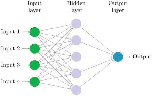
Artificial Neural Networks is an important supervised machine learning algorithm and is one of the powerful algorithm because of its ability to learn any functional relationship between one dependent and one or more independent variables. Moreover, it handles non-linear data effectively because of the use of activation functions. The purpose of activation function such as sigmoid, ReLU and tanh is to effectively handle the nonlinear relationship between the output variable and input variables. A typical ANN architecture consists of two layers (one hidden layer and one output layer). Conventionally, we don’t count input layer as an actual layer and therefore we always see a two-layer neural network as shown in (Figure 1).

Figure 1. Artificial neural network schematic.

Use of ANN has proved to be helpful in efficiently estimating the groundwater levels as compare to hydrologic simulation methods (Dash, Panda, Remesan, & Sahoo, 2010; Sahoo & Jha, 2013; Sahoo, Russo, Elliott, & Foster, 2017). The results from this hybrid ANN method showed that complex, nonlinear relationships among precipitation, temperature, streamflow, climate indices, irrigation demand, and groundwater levels could be represented and reproduced with the method. ANN has been used by Jain & Kumar, 2007 and Bougadis, Adamowski, & Diduch, 2005 to forecast water demand for monthly and weekly lead time respectively. ANNs has also been used in forecasting of energy generation from other renewable source like hydropower (French, Krajewski, & Cuykendall, 1992; Hammid, Sulaiman, & Abdalla, 2018; Lin & Chen, 2004; Luk, Ball, & Sharma, 2000; Pan & Wang, 2004; Ramirez, de Campos Velho, & Ferreira, 2005) and wind power (Barbounis & Theocharis, 2007; Hervás-Martínez et al., 2009; Kariniotakis, Stavrakakis, & Nogaret, 1996; Li & Shi, 2010; Welch, Ruffing, & Venayagamoorthy, 2009). Gomes & Castro, 2012 focused on predicting wind speed and power by statistical models like Artificial neural networks (ANN) and AutoRegressive moving average (ARMA) and concluded that ARMA, despite being more time consuming, performed better than ANN in terms of forecasting accuracy. Bugała et al., 2018 used ANN in short-term forecasting of electric energy from photovoltaic conversion. The independent variables (number of sunny hours, length of the day, air pressure, maximum air temperature, daily insolation, cloudiness) were selected on the basis of Pearson linear correlation coefficients. In Sauhats, Petrichenko, Broka, Baltputnis, & Sobolevskis, 2016, ANN has been used to hourly forecast hydropower reservoir inflow of a hydropower reservoir in Latvia using temperature, precipitation and historical water inflow.

Various types of neural networks are used in energy use analysis including feedforward networks and backpropagation networks. In Brown, Kharouf, Feng, Piessens, & Nestor, 1994; Brown & Matin, 1995 energy consumption is predicted using a feedforward network. Suykens et al., 1996 use a static non-linear neural network model to predict energy consumption. The work (Khotanzad & Elragal, 1999a) proposed a two-stage system for gas demand forecasting, the first stage comprising three ANN forecasters: a multilayer feed-forward network trained with backpropagation, a multilayer feedforward network trained with the Levenberg-Marquad algorithm, and a one-layer functional link network; and the second stage consisting of the nonlinear link functional ANN container which combines the three ANN forecasters of first stage. A similar two-stage approach was reprised in Khotanzad, Elragal, & Lu, 2000 in which the first stage combined two ANN forecasters with different topologies. The first forecaster is a multilayer feedforward architecture while the second one is a functional link ANN. In the second stage, the two individual forecasters of the first stage are combined together in order to achieve the final forecasting. Overall to achieve this, the authors explored eight different combination strategies – averaging, recursive least squares, fuzzy logic, feed-forward ANN, functional link ANN, temperature space approach, linear programming algorithm and modular neural networks.

Genetic algorithms (GA), based on a natural selection process that mimics biological evolution¹, are often used in conjunction with neural networks and other models to solve optimization problems. Because most of the other existing parameter estimation methods require additional information and are difficult to manage in practical applications, GA emerges as a better tool than other methods (e.g. direct search methods, Hooke-Jeeves method, Nelder-Mead method, gradient method) for estimating parameters in a non-linear regression models (Faradonbeh, Monjezi, & Armaghani, 2016; Nash & Walker-Smith, 1987; Nguyen, Reiter, & Rigo, 2014a; Pan, Chen, Kang, & Zhang 1995). In Pelikan & Simunek, 2005, genetic algorithms are used to optimize risk management of natural gas consumption to minimize losses of and maximize the profits of a particular gas distribution company. Aras, 2008 and Ervural, Beyca, & Zaim, 2016 present short-term forecasting of residential natural gas demand using genetic algorithms. In Forouzanfar, Doustmohammadi, Menhaj, & Hasanzadeh, 2010, an approach to forecast natural gas consumption for residential and commercial sectors by estimating the logistic parameters is performed using two different methods: non-linear programming and genetic algorithms.

GA has also been actively used in hydrological resource planning and management (Nicklow et al., 2009; Rani & Moreira, 2010). The study (Rani, Jain, Srivastava, & Perumal, 2013) presents an overview of GA applications to water resource problems such as optimization of water distribution system and reservoir system operation. In the recent past, Abkenar, Stanley, Miller, Chase, & McElmurry, 2015 used genetic algorithms for optimization of pump schedules in water distribution systems. Bi, Dandy, & Maier, 2015 proposed a new heuristic sampling method in improving the efficiency in application of genetic algorithm to water distribution systems. Wafae, Driss, Bouziane, & Hasnaoui, 2016 used genetic algorithm for optimization of operation in reservoir system in Morocco. Tayebiyan, Ali, Ghazali, & Malek, 2016 explored the use of genetic algorithm in optimizing reservoir operations under different water release policies in Cameron highland hydropower system, Malaysia.

3.1.3. Support vector machines

Support vector machine is the powerful supervised learning technique that is used for both classification and regression. Supervised learning approaches to prediction of solar power generation included use of linear least squares regression and support vector machines (SVM) using three different kernels – linear kernel, polynomial kernel, and radial basis function (RBF) kernel (Hossain, Oo, & Ali, 2012). The use of SVM with kernel functions is to map nonlinear data from input space to a higher dimensional space to make it linearly separable. The use of this kernel trick in SVMs have been further explored not only in other domains (Mohandes, Halawani, Rehman, & Hussain, 2004; Pai & Lin, 2005) but also in rainfall forecasting (Hong, 2008; Wang, Xu, Chau, & Chen, 2013) since hydropower generation is subjected to external factors like patterns in precipitation. Support vector machines (SVM) (Chang, 2014; Zeng & Qiao, 2011) has been applied successfully to short-term wind power forecasting. In addition to wind speed predictions, SVMs are applied to future water availability estimates and air and water quality prediction (Wang, Xu, & Weizhen, 2003). Linear least squares regression² techniques and SVM are used by Sharma, Sharma, Irwin, & Shenoy, 2011 to predict solar power generation based on weather forecasts. The potential of circuit-level electricity data for major household appliances such as clothwasher and dishwasher in water end use disaggregation is presented in Vitter & Webber, 2018. This involved an attempt to align electricity consumption data in the disaggregation tool. To classify water events, two different support vector machine classification models were used. The first model used input data with two features event volume and event duration. The second model used these features along with two more features that indicating coincident electricity consumption by a clothwasher or dishwasher. These additional features were used in order to address the problem of overlapping water events (Vitter & Webber, 2018) and unrelated water consumption events.

3.1.4. Decision trees

Decision trees are a supervised machine learning method used for classification and regression. The deeper the tree, the more complex the decision rules and the more fit the model.³ The advantages of this technique includes easy to understand, interpret and visualize while the disadvantages includes high variance that leads to overfitting problem. Energy use is also predicted using decision trees (Al-Gunaid, Shcherbakov, Skorobogatchenko, Kravets, & Kamaev, 2016; Tso & Yau, 2007). Decision tree models can produce rules or logic statements that are easy to interpret, but they don’t perform as well as Neural Networks for non-linear data and they tend to be susceptible to noise (Curram & Mingers, 1994).

3.1.5. Time series analysis models

Use of time series models that typically includes Box-Jenkins models have been presented in several studies related to forecasting energy demand. For example, ARIMA is used in forecasting monthly or annual natural gas consumption in Akkurt, Demirel, & Zaim et al., 2010 and Erdogdu, 2010. Additionally, Akkurt et al., 2010 show that an extension of ARIMA, seasonal autoregressive integrated moving average (SARIMA), can outperform the other models for monthly forecasting, and that further double exponential smoothing can produce optimal results for annual forecasting. The Structure Time Series Model (STSM) is also employed to forecast annual energy demand (as in Dilaver, Dilaver, & Hunt, 2014, which includes in its analysis the effect of various determinants such as income, natural gas price, and underlying energy demand trends (1978–2011) on natural gas demand. A STSM is a model formulated directly in terms of components of interest in a time series, and which has a direct interpretation. In such a model, the trend component is flexible enough to allow response to changes in the general direction, the seasonal component can respond to changes in the seasonal pattern, and these components are treated as stochastic–driven by random disturbances (Harvey, 1990).

The study (Hill, McMillan, Bell, & Infield, 2012) presented the application and use of univariate and multivariate Autoregression Moving Average (ARMA) models to geographically dispersed wind speed data in forecasting wind power. Huang, Huang, Gadh, & Li, 2012 used Autoregression Moving Average (ARMA) and persistence model to forecast future solar generation within the region of University of California, Los Angeles (UCLA). While evaluating the models, ARMA was found to be performing better in short- and medium-time forecasting while persistence model performed better under very short duration.

3.1.6. Comparative analysis of supervised techniques

The supervised learning techniques are often compared for the same problem in order to evaluate the techniques on prediction accuracy and generalizability error. The study (Khan & Coulibaly, 2006) presents a performance comparison of SVM, ANN, and traditional seasonal autoregressive model (SAR) in forecasting of water level of a lake. In this case, SVM was shown to be competitive with the other two methods. The study (Herrera, Torgo, Izquierdo, & Pérez-Garca, 2010) compared the performance of different models: artificial neural networks (ANN)) (Bishop, 1995; Bougadis et al., 2005; Maier & Dandy, 2000; Zhang & Qi, 2005), projection pursuit regression (PPR) (Dahl & Hylleberg, 2004; Friedman & Stuetzle, 1981; Storlie & Helton, 2008a), multivariate adaptive regression splines (MARS) (Friedman & Stuetzle, 1981; Hastie & Tibshirani, 1990; Moisen & Frescino, 2002), support vector regression (SVR) (Cristianini & Shawe-Taylor, 2000; Karatzoglou, 2006; Karatzoglou, Meyer, & Hornik, 2005; Smola & Schölkopf, 2004; Vapnik, 2013; Vapnik & Vapnik, 1998), random forests (Breiman, 2001), and a weighted pattern-based model (Alvisi, Franchini, & Marinelli, 2007; Härdle, Liang, & Gao, 2012; Herrera et al., 2010) used for short-term water demand forecasting for a south-eastern city in Spain. Predictors used for the comparison were water demand at current hour, previous hour, and target hour in previous week; temperature; wind velocity; atmospheric pressure; and rainfall. Monte Carlo estimation method is used to evaluate the models on the data. The Monte Carlo methods depends on the repetition of a simulation experiment to obtain estimates of any variable. Results of the Monte Carlo comparisons for all of the models showed that SVM, Random Forests, PPR and MARS perform better than ANN and the weighted pattern-based model. In light of these results, Tu-Qiao, 2006 and Chen & Zhang, 2006 propose a added Bayesian (predictions made based on prior knowledge) and a least squares SVM, respectively, for forecasting hourly demand. A comparative study (Msiza, Nelwamondo, & Marwala, 2007) is presented that compares the performance of artificial neural network (ANN) and support vector machine (SVM) for forecasting water demand and is observed that the ANN performs better than SVM in better generalizing the unseen data.

The study (Danades, Pratama, Anggraini, & Anggriani, 2016) compares a non-parametric K-Nearest Neighbor (KNN) algorithm and a SVM algorithm in the classification of water quality. It starts by defining a pollution index based on parameters established in previous research. Next, they categorize the dependent variable (predictand) using labels: Good Condition, Lightly Polluted, Medium Polluted and Heavily Polluted. They characterize the independent (predictor) variables with attributes: Total Suspended Solids (TSS), Dissolved Oxygen (DO), Chemical Oxygen Demand (COD), Biochemical Oxygen Demand (BOD), Total Phosphate, Fecal Coliform and Total Coliform. Training and test datasets are apportioned, then the KNN algorithm is run to classify objects based on the learning data located closest to the object. The learning data are projected into many-dimensional space in which each dimension represents features of the data. Next, the Support Vector Machine (SVM) algorithm is run with the data, within a hypothesis space in the form of linear functions in a high-dimensional feature space which makes the use of kernel functions. The result of the experiment shows that SVM performed much better (92.4% accuracy) than the KNN (71.28% accuracy). Several studies (Adamowski, 2008; Adamowski et al., 2012; Caiado, 2009) have compared ANN with the traditional linear regression models, finding ANN to produce a better forecast than the regression models for water demand forecasting.

Daily forecasting of energy consumption is researched in Taspnar, Celebi, & Tutkun, 2013, in which a comparison of the performance of different models is considered with respect to a specific dataset consisting of air temperature, cloud cover, relative humidity, atmospheric pressure and wind speed as predictors. Time series analyses performed include the Box-Jenkins variant, seasonal autoregressive integrated moving average with exogenous inputs (SARIMAX), and two ANNs, one combined using a radial basis function (RBF), as its hidden layer, and the other as a multilayer perceptron (MLP), described next. A MLP is a type of feedforward artificial neural network which consists of at least three layers of nodes and uses a supervised learning technique called backpropagation for training. Results from the Taspnar et al., 2013 study indicate that the MLP architecture performs optimally on energy consumption given meteorological predictors consists of five input, eight hidden, and one output neurons.

Comparisons among multiple regression models, time series models (ARMAX) and artificial neural networks for energy consumption forecasts were made in (Demirel et al., 2012; Werbos, 1988). Results from one study (Demirel et al., 2012) showed that an artificial neural network with backpropagation outperforms multiple regression and the ARMAX model in terms of root mean square error (RMSE) and mean absolute percentage error (MAPE); however, ARMAX provides the best results in terms of mean absolute deviation (MAD). The other research study (Werbos, 1988) showed that artificial neural networks perform much better than time-series and regression models in forecasting energy consumption.

Because of the advantages and limitations of all of these approaches, some researchers have chosen to combine them. For example, Tso & Yau, 2007 used a stepwise regression model, a multi layer perceptron model and a decision tree model within the SAS Enterprise Miner Inc., 2003 statistical framework to determine total weekly electricity consumption (in KWh) using housing type, household characteristics and appliance ownership as the potential factors influencing the electricity energy consumption. Input for these models was collected using a questionnaire-diary method covering the details pertaining to appliances’ ownership and power ratings among participating households during both summer and winter. Results were compared with the model performance measure based on the square root of averaged square error (RASE). It was found that in the summer phase, the decision tree model performs slightly better as compared to the other models while in the winter phase neural network performs slightly better than the other two models.

3.2. Unsupervised learning

Unsupervised learning approaches are based on finding hidden structure from unlabeled data. Unlike supervised learning approach where we have a known labeled data of input and output variables, in the unsupervised learning we learn the hidden patterns, associations, similarities between the inputs without any known output variable. Commonly used techniques of this approach in the energy-water nexus space comprises of clustering techniques based on hierarchical (Helmbrecht, Pastor, & Moya, 2017; Noiva, Fernández, & Wescoat, 2016), density (Zhang, Du, Yao, & Ren, 2016) and partitional (Grubert, 2016; Pastor-Jabaloyes, Arregui, & Cobacho, 2018; Zou, Zou, & Wang, 2015) clustering method. Other techniques used in energy water nexus are Principal component analysis (PCA) citeplam2008principal, ndiaye2011principal and Hidden Markov models (HMM) (Nguyen, Stewart, & Zhang, 2013a, 2014b; Nguyen, Stewart, Zhang, & Jones, 2015; Nguyen, Zhang, & Stewart, 2013b). Table 4 shows unsupervised techniques used within the scope of energy-water nexus.

Hierarchical clustering is used in conjunction with business rule techniques in Helmbrecht et al., 2017 in developing a solution that monitors water supply systems for events detection and water resource management thereby increasing the energy efficiency. Noiva et al., 2016 used hierarchical cluster analysis to analyze water supply and demand for 142 cities around the world using MIT Urban metabolism database. This involved identifying cities having similar characteristics in water and energy demand. Density-based clustering such as Density-Based Spatial Clustering of Applications with Noise (DBSCAN) algorithm has been in conjunction with kernel density estimation in Zhang et al., 2016 for evaluating and clustering maps in the groundwater wells located in red beds of three regions in China. Use of partitional-based clustering can be seen in Grubert, 2016, where the authors employed K-means clustering technique for improving the estimates for comparing hydroelectric power’s water consumption to that of other energy sources using entire United States population of hydroelectric dams with estimates for net and gross evaporation at national and regional level. Another example of using K-means clustering can be seen in the study (Zou et al., 2015), based on water quality analysis of the Haihe River using data obtained by the monitoring network for the period (2006–2013).

With the growing pace of energy demand, it has become important to manage energy supply in an efficient manner through monitoring and assessing the pattern of end energy use. For example, how the information on aggregate household electricity power consumption can be decomposed at individual appliance level. To answer this, researchers have developed Non-Intrusive Appliance Load Monitoring (NIALM) algorithms. NIALM based on machine learning methods includes unsupervised learning algorithms like Hidden Markov Models studied in Johnson & Willsky, 2013; Kolter & Jaakkola, 2012; Parson, Ghosh, Weal, & Rogers, 2014. Although, these algorithms have shown good results in energy use disaggregation, they have been limited in handling appliances in multiple operating modes simultaneously and reconstructing the trajectories of power consumption over time. This limitation has been addressed through a novel sparse based optimization approach (Piga, Cominola, Giuliani, Castelletti, & Rizzoli et al., 2016) where disaggregation problem is being treated as least-square minimization problem with a convex penalty term with information on time-of-day probability for each appliance and an assumption that power consumption of an appliance is piecewise constant over time.

Several studies (Nguyen et al., 2013a, 2014b, 2015, 2013b) has shown a good potential for water end use disaggregation and classification of water consumption events through combining machine learning techniques such as Hidden Markov Models (HMM), Dynamic Time Warping (DTW) and Artificial Neural Networks. This approach was limited in its universal usability and compatibility since the data used for training the algorithms came from a particular water meter data of some specific geographical location where water consumption habits of users tends to be similar in nature. In order to address this, another clustering based algorithm, Partition Around Medoids (PAM) (Reynolds, Richards, de la Iglesia, & Rayward-Smith, 2006) has been used in disaggregating water end use events in Pastor-Jabaloyes et al., 2018. This involved the disaggregation process where all the water consumption events are decomposed into single-use or uncertain type of events which is then used to group single use water events through PAM with a hypothesis that similar characteristics of single use events correspond to the same cluster or group of end use.

Principal component analysis (PCA), another useful unsupervised learning based feature transformation technique that is used to explore variations in inputs or independent variables. It is a standard data reduction technique that forms a new set of orthogonal variables called principal components that are linear composites of the original variables. This technique helps in representing original data into low-dimensional space by identifying linear combination set of features that accounts for maximal variance and are simultaneously uncorrelated. PCA can be applied to processes related to both the electricity sector and the water sector (e.g. Carle, Halpin, & Stow, 2005; Evans, Guthrie, & Videbeck, 2008; Lam, Wan, Cheung, & Yang, 2008; McManamay et al., 2017; Ndiaye & Gabriel, 2011; Parinet, Lhote, & Legube, 2004). Specifically, McManamay et al., 2017 use principal components to calculate a cumulative hydrologic alteration index (from a seasonal hydrologic alteration index) for 250 nonreference hydrological gages based on multidimensional measurements. Indices describe different aspects of the hydrograph, including the magnitude, timing, frequency, duration, and rate of change in flow. This technique has also been applied extensively to rainfall calculations (e.g. Basalirwa, 1995; Dyer, 1975; Munoz-Diaz and Rodrigo, 2004; Ogallo, 1989).

3.3. Ensemble learning

Ensemble learning combines various machine-learning models called “base learners” in order to solve a problem. Usually, in order to get the ensemble learning to work, we firstly, generate a number of base learners either in sequential or parallel in such a way that generation of base learners has influence on the generation of the subsequent learners (Zhou, 2009) and then secondly, we combine the predictions of those base learners in order to get the prediction output of the ensemble model. The combination schemes of the base learners can be either voting for classification problem or weighted averaging for regression problem. Ensemble methods has the advantage of performing better than individual learning algorithms since it reduces the variance and keep the balance of bias-variance in control which helps in giving better generalizability on unseen data. Common methods includes Bootstrap aggregation (Bagging), Boosting, random forests among many others (Dietterich, 2000). Table 5 shows some ensemble learning and hybrid techniques that have been used in the past for predicting energy resource systems.

3.3.1. Bayesian model averaging

There are considerable limitations to employing a single model in predicting future energy consumption because of the level of uncertainty associated with model structure and parameters. Thus, a hybrid model approach is taken in Zhang & Yang, 2015 in which natural gas consumption is forecast by Ensemble Bayesian model averaging (BMA). Bayesian model averaging (BMA) allows the uncertainty of the model itself to be considered in the statistical analysis while it computes the posterior model probability. This approach reduces the uncertainty inherent in individual models. The BMA method shows better prediction accuracy than individual models like grey prediction, linear regression and artificial neural networks, because as it runs it evaluates the performance

using RMSE and mean absolute percentage error (MAPE, $M=\frac{100}{n}\sum _{t=1}^n\left|\frac{A_t-F_t}{A_t}\right|$ with $A_t$ = measured

value, $F_t$ = forecast value and $n$ = total number of samples). BMA can assume different values for parameters (GDP, urban population, energy consumption, industrial structure, etc.) under different scenarios (Zhang & Yang, 2015).

3.3.2. Random forests

Random forests, a supervised learning technique that is built as an ensemble of decision tree is seen to be useful for water (Chen, Long, Xiong, & Bai, 2017; Lin et al., 2015; McManamay, 2014) and energy (Lahouar & Slama, 2017) related application areas. One great advantage of this technique is that it can be useful in both regression and classification problems (Liaw et al., 2002). The method is capable of high classification or regression accuracy, characterization of complex predictor variable interactions, flexible analytical technique selection, and appropriate missing value handling (Breiman, 2001).

The study (McManamay, 2014) applied this technique to hydrological networks to quantify and generalize hydrologic responses to dam regulation, and the authors found that this method is capable of generalizing the directionality of hydrologic responses to dam regulation and providing parameter coefficients to inform future site-specific modeling efforts. Chen et al., 2017 proposed a model, composed of random forests regression and wavelet transform, for predicting daily urban water consumption. This model more accurately predicted water consumption as compare to other individual models such as random forests regression and feed-forward neural network.

Use of random forest has also been carried out in predicting energy generation and consumption. Lin et al., 2015 used random forest modeling as a modeling technique in seasonal analysis and prediction of wind energy. It used AutoRegressive Moving Average (ARMA) model structure to represent wind speed and direction. The functional form of the model structure was then determined using random forest. The modeling accuracy of random forest was compared with Support Vector Regression (SVR) and Artificial neural network (ANN) and it was found that random forests outperformed both SVR and ANN. Using random forest to forecast hour-ahead wind power has been studied in Lahouar & Slama, 2017. This involved selection of important weather factors such as wind speed and wind direction on the basis of correlation and importance measures. The study (Ma & Cheng, 2016) used random forest in exploring the influence of 171 features that are related to the energy use intensity (EUI) of residential buildings. The influential features describing the buildings, households, education, environment, surrounding and transportation were identified based on out-of-bag estimation in random forest.

3.3.3. Other hybrid models

In Tiwari & Adamowski, 2014, 2017, the authors explored the hybrid approach for modeling weekly and monthly urban water demand forecasting in cases where data availability is limited (Donkor, Mazzuchi, Soyer, & Alan Roberson, 2012; Tiwari & Chatterjee, 2010). This approach comprised of wavelet-bootstrap ANN (WBANN), which resulted in handles the uncertainty associated with forecast on urban water demand by mimicry of randomness, thereby reducing the uncertainty in variance (Efron, 1992). A hybrid model using firefly algorithm (FA) (Yang & He, 2013), a nature-inspired optimization tool into least square support vector regression (LSSVR) for predicting hydropower consumption has been proposed in Tang et al., 2015. The optimization tool was used to determine the task of determination of parameters in LSSVR. Hong, 2008 discussed hybrid forecasting technique combining RANN and SVM regression with a chaotic particle swarm optimization algorithm (RSVRCPSO) for forecasting rainfall forecasting. Specifically, Jordan Networks (Jordan, 1986), a variant of RANN is employed as a base to construct the recurrent SVR models. RSVRCPSO holds a particular advantage over the other analytical tools in terms of its ability to (i) capture electricity load data patterns easily, (ii) determine suitable parameters (using the swarm optimization algorithm) that can forecast typhoon rainfall depth data accurately, and (iii) perform structural risk minimization (rather than relying on minimizing training errors). Advantages of this hybrid approach are determination of better, accurate and more reliable results important not only for analyzing hydropower generation, but also in preparation for sudden flood events and recovery of economic and human losses. Ren, Suganthan, & Srikanth, 2015 reviewed some wind power and solar irradiance forecasting with ensemble methods. Short-term forecasting of wind speed and wind power based on wavelet method and improved time series method (ITSM) is presented in Liu et al., 2010. Advantage of this hybrid approach consisted of improved forecasting accuracy without the need to increase the computational model cost. In Peng et al., 2017, the authors used a hybrid two-stage decomposition algorithm embedded with complementary ensemble empirical mode decomposition with adaptive noise (CEEDMAN) (Torres, Colominas, Schlotthauer, & Flandrin, 2011), variational mode decomposition (VMD) (Dragomiretskiy & Zosso, 2014), AdaBoost.RT (Solomatine & Shrestha, 2004) and extreme learning machine (ELM) (Huang, Zhu, & Siew, 2004) for multistep forecasting of wind speed. The algorithm also showed considerable improvement in accuracy due to its capability in capturing non-linear characteristics of wind speed time series in comparison to other methods (Peng et al., 2017).

Use of wavelet recurrent backpropagation network (RBPN) to forecast solar irradiance is presented in Cao & Cao, 2006, 2005 where for one-day ahead forecasting the wavelet RBPN performed better than the RBPN without any wavelet decomposition. A hybrid approach to forecast solar power with effective accuracy is presented in Hossain et al., 2012. It involved the ensemble generation, which comprised of different regression algorithms such as linear regression, multilayer perceptron, support vector machine among others (Hossain et al., 2012). Azimi et al., 2016 proposed a hybrid approach to forecast solar radiation for different time horizons. This approach combined a novel clustering method, TB K-means with time-series analysis, a novel clustering selection algorithm and a multilayer perceptron neural network. The performance of this hybrid approach is then evaluated and compared with different variants of k-means algorithm using different solar datasets and the results shows that this approach gives better forecasting results. Hussain & AlAlili, 2017 used a hybrid modeling approach to estimate solar radiation. This involved the combination of wavelet multiresolution analysis and artificial neural networks. The wavelet multiresolution analysis is applied in order to decompose complex input signals into different frequency and time resolutions. These decomposed signals or time-series were then modeled by four different ANN models (multilayer perceptron (MLP), adaptive neuro-fuzzy inference system (ANFIS), nonlinear autoregressive recurrent exogenous neural network (NARX), and generalized regression neural networks (GRNN)). The modeled time series were then combined to estimate the original signal. This hybrid approach was shown to outperform traditional standalone ANNs in terms of coefficient of determination ($R^2$), root mean square error (RMSE), mean bias error (MBE), mean absolute percentage error (MAPE), and t-statistics.

3.4. Reinforcement learning

Reinforcement learning approach is based on the learning of agents’ behavior by getting a feedback from the environment. It differs from both supervised learning and unsupervised learning approach in a considerable manner. In supervised learning, we have the labeled set of training data and learning is performed based on this limited set of input and outputs that may not cover the exhaustive set of situations that may be unseen in future. This set of learning may not be suitable for interactive problems (Sutton & Barto, 1998) in which reinforcement learning tends to perform better since it constantly interacts with the environment in getting responses for its actions. Similarly, Unsupervised learning also limits in finding structural patterns within the examples in a data while reinforcement learning approach aims at maximizing the reward signals concerning interacting of agent with its environment. The environment is typically formulated as Markov decision process and example of which can be seen in (Nanduri and Saavedra-Antolínez, 2013) where dynamic competition in wholesale electricity markets has been simulated by Competitive Markov Decision models (CMDP) in which stochastic approximation-based reinforcement learning (RL) algorithms have been employed. The advantage of using CMDP is that it allows capture of the inherent dynamic and noncooperative nature of electricity market participants under stochastic demand conditions. Impacts of different forms of joint water and carbon taxes and extreme climatic events such as drought are investigated on the sampled electricity network. The different tax scenarios considered are: (1) ramping up, (2) grandfathering, and (3) uniform adaption. Due to nonconsensus in deciding a better approach amongst tax scenarios, the model determines the impact of different tax scenarios on complex wholesale electricity market operations. Because long-term disruption of water supply is significantly attributed to climate change (DOE, 2007) and water supply plays an important part in power generation, the impact of water shortage on operational performance of power generators is shown.

4. Machine learning opportunities for the energy-water nexus

Energy and water is inherently linked with climate change and so it is require to get useful insights into past and future climate patterns; however, this insight would be pretty difficult to develop (Burkett et al., 2013). Interactions between water and energy have considerable variations across different regions due to factors like climate, population density, and level of economic development among others (DOE, 2014). It is important for us to model the water-system interactions in a way that effectively handles uncertainties of both human earth and natural earth systems (DOE, 2014). Moreover, it would be require to see the impact on water supply as a result of change in energy demands or the impact on energy supply in changing water demands.

Therefore, it is required for us to build the machine learning models in order to predict the water and energy system resources tackling changes in different socioeconomic and biophysical variables and uncertainty in predictions simultaneously. In the following, we describe possible opportunities in machine learning direction for solving energy-water nexus problems.

4.1. Mining patterns and relationships in data

Uncovering patterns and relationships between variables of interactions relevant to energy-water nexus using data mining techniques (Berkhin, 2006; Dunham & Ming, 2003; Han, Pei, & Kamber, 2011) will be significantly important. For example, it would be better to explore an association or relation between precipitation on water discharge through hydroelectric power plant and subsequently electricity generation through data mining techniques. Using spatial (Koperski, Adhikary, & Han, 1996), temporal (Antunes & Oliveira, 2001) and spatio-temporal data mining methods (Shekhar et al., 2015) in discovering useful knowledge from existing datasets may prove to be useful for further research analysis and work. For example, there could be a possible clustering of county-level or state-level regions that exhibit similar trends and characteristics in water-energy resource interactions. Moreover, it can also lead to outlier detection in a way that a particular region doesn’t confirm to the association to and major clustering groups.

Spatio-temporal data mining has various broad applications in ecology, environment management and climatology (Shekhar et al., 2015). Additionally, there is a potential of employing network-mining techniques (Galloway & Simoff, 2006) which can identify any networks between large number of data variables within interacting nexus entities like, for example, energy generation and water distribution. For Energy-water nexus, an integrated linear optimization models to track resource flow throughout energy and water systems using harmonization of varying spatio-temporal data scales is presented in Khan et al., 2018.

4.2. Addressing heterogeneity in data

Data in Energy-water nexus comes from disparate sources and differs in terms of modality and spatio-temporal resolution. To address this issue, it could be better to use kernel methods (Filippone, Camastra, Masulli, & Rovetta, 2008; Ralaivola, 2004) as these methods uses various forms of similarity or kernel functions that incorporates different forms of spatial, temporal or network dependencies (Galloway & Simoff, 2006). Moreover, they can be used to build novel predictive, classification and clustering models that can be used to predict future values of target variables and account for uncertainty propagation in predictions. These methods have been used to understand changes in land biomass using satellite imagery (Chandola & Vatsavai, 2010, 2011).

4.3. Predicting energy-water nexus variables

Forecasting a variable ahead in time based using the historical data is an important task in analyzing the behavior and exploring trends in variables concerned with energy-water nexus. For instance, forecasting short-, medium-, and long-term trends for water consumption in thermoelectric power generation (Feeley III et al., 2008; Van Vliet et al., 2016) or energy consumption in wastewater treatment (Clark, 2018; Longo et al., 2016) would be useful in carrying out water and energy related planning decisions. The study (Yin, Jia, Wu, Dai, & Tang, 2018) used Artificial Neural Networks (ANN) to forecast water and energy demand in Wuxi City, China. The forecasting was consistent with the local planning data, and therefore it was concluded that the model can prove to be useful in providing strategies for development of water and energy in that region.

4.4. Modeling unobserved variables

In energy-water nexus data, modeling the known or observed variable would be an easier task to accomplish relatively to unobserved variables or variables having missing data. To achieve the task of modeling unobserved or latent variable use of latent variable models (Bishop, 1998) such as factor analysis model or finite mixture model (McLachlan & McGiffin, 1994) would be useful approaches. These model aims at indirectly inferring properties of latent variable by connecting them to observed variables. Applications of latent variable models include longitudinal analysis (Verbeke, 1997) and spatial statistics (Rue & Held, 2005).

4.5. Integration of models

It would be difficult to use one common model for building relationships between variables among different resource systems of energy-water nexus that varies greatly over time and space. There would be cases where a model that is producing good results at a particular spatial and temporal scale may not be able to produce effective results when these scales are changed. In such a scenario, it is important to integrate models that vary spatiotemporally using ensemble learning methods (Dietterich, 2000) or hybrid approaches (Krasnopolsky & Fox-Rabinovitz, 2006). Ensemble learning methods like bagging and boosting has the advantage of averaging the bias, reducing the variance and avoid the problem of overfitting which helps in providing better generalizability in predictions on unseen data. It could be also better to find ways to integrate data driven models with process based models in giving better results (Karpatne et al., 2017; Kinnebrew, Segedy, & Biswas, 2017; Wang, Wu, & Xiao, 2017) as this integration would help takes advantage of combining data-driven knowledge with knowledge of scientific principles.

4.6. Deep Learning

Deep Learning is a new evolving field of machine learning and has found its use in many application domains like computer vision (He, Zhang, Ren, & Sun, 2014; Szegedy et al., 2015; Zeiler & Fergus, 2014) and natural language processing (Bengio, Ducharme, Vincent, & Jauvin, 2003; Collobert and Weston, 2008; Pennington, Socher, & Manning, 2014; Rumelhart, Hinton, & Williams, 1986). In terms of performance, deep learning outperforms the traditional learning algorithms due to its ability to automatically extract features and producing good prediction results. In the context of energy-water nexus scope, Nguyen et al., 2017 used high-resolution water energy consumption data to improve water-end use disaggregation through applying a range of pattern recognition approaches which includes a Deep Neural Network – stacked autoencoder network along with Dynamic Time Warping (DTW) algorithm and Hidden Markov Models (HMM). Much of the work has been done in related climatic science, which comes within the scope of energy-water-climate nexus due to availability of labeled datasets, computation advancements (Deng et al., 2009). However, in order to better model energy-water interactions it is important to understand climate variability as it greatly drives this interaction because of an inherent uncertainty associated with uneven occurrence of extreme events which disrupts the water cycle and subsequently disturbing the ecological balance of energy-water nexus.

In order to handle large set of extreme climate patterns and events, deep learning methods have been implemented in Iglesias, Kale, & Liu, 2015; Liu et al., 2016. In Iglesias et al., 2015 a preliminary examination is carried out using multitask neural network (MTNN) in order to explore the potential role of deep learning in detecting extreme climate events. MTNN is used to predict heat waves using time-series data that includes variables related to solar radiation and atmospheric radiations temperature and weather. The research work (Liu et al., 2016) described the use of deep convolutional neural network (CNN) for tackling the extreme weather events – tropical cyclones, atmospheric rivers and weather fronts – detection in climate datasets. Here, deep CNN that consists of four learnable layers that includes two convolution layers and two fully connected layers. Each convolution layer is followed by a Rectified Linear Unit (ReLU) and a max pooling layer. Amongst the two fully connected layers, the first layer is followed by ReLU activation function as characteristic while the second layer or final fully connected layer has logistic activation function as nonlinearity. This configuration demonstrates a fair accuracy of 89%–99% in detecting and classifying extreme events – tropical cyclones, atmospheric rivers and weather fronts. Recurrent Artificial Neural Networks (RANN/RNN) (Elman, 1990; Jordan, 1986; Kechriotis, Zervas, & Manolakos, 1994; Tsoi & Back, 1994; Williams & Zipser, 1989). In RANN, future inputs to the network are derived from past outputs. RANNs are based on feed-forward artificial neural networks, and include established links between layers. Their utility in forecasting of long-term potential energy inflows has been shown for hydropower operations planning by Coulibaly, Anctil, & Bobée, 2000. Because of the nonstationarity of rainfall trends due to ongoing changes in climate, dynamic SVMs can be used to gain understanding of these changing patterns (Cao & Gu, 2002).

5. Conclusions

Maintaining sustainable supplies of water and energy for future generation is the significant challenge in energy water nexus. Due to increasing competition for limited water and energy resources, it is important for the decision and policy makers to act in a prudent manner while formulating policies and decisions on managing these resources. This paper presented the possible challenges and opportunities for machine-learning community in tackling energy-water nexus issues.

Although, machine learning based techniques have been employed in modeling individual resource water and energy systems, there is high potential in these techniques in providing future values for water and energy interactions across varying space and time scale taking account of uncertainty. This would be helpful in gathering key information and results that will help different stakeholders, resource managers, policy makers, and decision makers to invest in formulating policies and decisions that provide easy ways to tackle problems that may arise in the future. It will also be useful for the machine-learning techniques to provide predictions with better generalizability on unseen data in order to get more reliable and accurate future water and energy resource projections. The results should be easily interpretable and communicable to the energy-water nexus researchers.

There is also an urge for relevant stakeholders, science and machine-learning researchers to work in a cooperative and collaborative manner. It is important for energy and hydrological researchers to provide key questions relevant to water-energy interactions. Similarly, machine-learning researchers will provide useful analysis and develop novel methods for providing future projections to key variables in this nexus. Thus, the synergistic and symbiotic relationship between machine learning world and energy-water nexus world will prove to be fruitful and beneficial in the long-term goal of tackling energy water nexus.

Acknowledgements

This manuscript has been authored by employees of UT-Battelle, under contract DE-AC05-00OR22725 with the US Department of Energy. The authors would also like to acknowledge the financial and intellectual support for this research by the Integrated Assessment Research Program of the US Department of Energy’s Office of Science, Biological and Environmental Research. This work is supported in part by NSF ACI-1541215.

Disclosure statement

No potential conflict of interest was reported by the authors.

Notes

1. https://www.mathworks.com/discovery/genetic-algorithm.html.

2. http://www.itl.nist.gov/div898/handbook/pmd/section1/pmd141.htm.

3. http://scikit-learn.org/stable/modules/tree.html.

References

- Abkenar, S. M. S., Stanley, S. D., Miller, C. J., Chase, D. V., & McElmurry, S. P. (2015). Evaluation of genetic algorithms using discrete and continuous methods for pump optimization of water distribution systems. Sustainable Computing: Informatics and Systems, 8, 18–23.
- Abuella, M., & Chowdhury, B. (2015). Solar power probabilistic forecasting by using multiple linear regression analysis. In SoutheastCon 2015 (pp. 1–5). IEEE.
- Adamowski, J., Fung Chan, H., Prasher, S. O., Ozga-Zielinski, B., & Sliusarieva, A. (2012). Comparison of multiple linear and nonlinear regression, autoregressive integrated moving average, artificial neural network, and wavelet artificial neural network methods for urban water demand forecasting in montreal, canada. Water Resources Research, 48(1).
- Adamowski, J. F. (2008). Peak daily water demand forecast modeling using artificial neural networks. Journal of Water Resources Planning and Management, 134(2), 119–128.
- Ahmad, A., Hassan, M., Abdullah, M., Rahman, H., Hussin, F., Abdullah, H., & Saidur, R. (2014). A review on applications of ann and svm for building electrical energy consumption forecasting. Renewable and Sustainable Energy Reviews, 33, 102–109.
- Akkurt, M., Demirel, O. F., Zaim, S. (2010). Forecasting turkey’s natural gas consumption by using time series methods. European Journal of Economic and Political Studies, 3(2), 1–21.
- Al-Garni, A. Z., Zubair, S. M., & Nizami, J. S. (1994). A regression model for electric-energy-consumption forecasting in eastern saudi arabia. Energy, 19(10), 1043–1049.
- Al-Gunaid, M. A., Shcherbakov, M. V., Skorobogatchenko, D. A., Kravets, A. G., & Kamaev, V. A. (2016). Forecasting energy consumption with the data reliability estimation in the management of hybrid energy system using fuzzy decision trees. In Information, Intelligence, Systems & Applications (IISA), 2016 7th International Conference (pp. 1–8). Chalkidiki, Greece: IEEE.
- Alvisi, S., Franchini, M., & Marinelli, A. (2007). A short-term, pattern-based model for water-demand forecasting. Journal of Hydroinformatics, 9(1), 39–50.
- Al-Zahrani, M. A., & Abo-Monasar, A. (2015). Urban residential water demand prediction based on artificial neural networks and time series models. Water Resources Management, 29(10), 3651–3662.
- Antunes, C. M., & Oliveira, A. L. (2001). Temporal data mining: An overview. KDD Workshop on Temporal Data Mining, 1, 1–13.
- Arandia, E., Ba, A., Eck, B., & McKenna, S. (2015). Tailoring seasonal time series models to forecast short-term water demand. Journal of Water Resources Planning and Management, 142(3), 04015067.
- Aras, N. (2008). Forecasting residential consumption of natural gas using genetic algorithms. Energy Exploration & Exploitation, 26(4), 241–266.
- Arbués, F., Garca-Valiñas, M. Á., & Martnez-Espiñeira, R. (2003). Estimation of residential water demand: A state-of-the-art review. The Journal of Socio-Economics, 32(1), 81–102.
- Azimi, R., Ghayekhloo, M., & Ghofrani, M. (2016). A hybrid method based on a new clustering technique and multilayer perceptron neural networks for hourly solar radiation forecasting. Energy Conversion and Management, 118, 331–344.
- Baki, S., & Makropoulos, C. (2014). Tools for energy footprint assessment in urban water systems. Procedia Engineering, 89, 548–556.
- Barbounis, T., & Theocharis, J. B. (2007). Locally recurrent neural networks for wind speed prediction using spatial correlation. Information Sciences, 177(24), 5775–5797.
- Barnett, V., & Lewis, T. (1974). Outliers in statistical data. Hoboken, NJ: Wiley.
- Basalirwa, C. (1995). Delineation of uganda into climatological rainfall zones using the method of principal component analysis. International Journal of Climatology, 15(10), 1161–1177.
- Bengio, Y., Ducharme, R., Vincent, P., & Jauvin, C. (2003). A neural probabilistic language model. Journal of Machine Learning Research, 3(Feb), 1137–1155.
- Berkhin, P. (2006). A survey of clustering data mining techniques. In Grouping multidimensional data (pp. 25–71). Berlin, Heidelberg: Springer.
- Bhagwat, P. P., & Maity, R. (2013). Hydroclimatic streamflow prediction using least square-support vector regression. ISH Journal of Hydraulic Engineering, 19(3), 320–328.
- Bi, W., Dandy, G. C., & Maier, H. R. (2015). Improved genetic algorithm optimization of water distribution system design by incorporating domain knowledge. Environmental Modelling & Software, 69, 370–381.
- Bi, Y., & Jeske, D. R. (2010). The efficiency of logistic regression compared to normal discriminant analysis under class-conditional classification noise. Journal of Multivariate Analysis, 101(7), 1622–1637.
- Bianco, V., Scarpa, F., & Tagliafico, L. A. (2014). Scenario analysis of nonresidential natural gas consumption in Italy. Applied Energy, 113, 392–403.
- Bishop, C. M. (1995). Neural networks for pattern recognition. New York, NY, USA: Oxford University Press, Inc.
- Bishop, C. M. (1998). Latent variable models. In Learning in graphical models (pp. 371–403). Springer.
- Boersma, T., Andrews-Speed, P., Bleischwitz, R., Johnson, C., Kemp, G., & VanDeveer, S. D. (2014). Want, waste or war?: The global resource nexus and the struggle for land, energy, food, water and minerals. Abingdon, UK: Routledge.
- Bougadis, J., Adamowski, K., & Diduch, R. (2005). Short-term municipal water demand forecasting. Hydrological Processes, 19(1), 137–148.
- Breiman, L. (2001). Random forests. Machine Learning, 45(1), 5–32.
- Britt, E. (2018). Hurricanes Harvey and Irma: Electric industry impacts, restoration, and cost recovery. Technical report. http://www.dwmrlaw.com/wp-content/uploads/2018/04/ABA_INFRA57-1.pdf.
- Brown, R. H., Kharouf, P., Feng, X., Piessens, L. P., & Nestor, D. (1994). Development of feed-forward network models to predict gas consumption. In Neural Networks, 1994. IEEE World Congress on Computational Intelligence., 1994 IEEE International Conference (Vol. 2, pp. 802–805). Orlando, FL, USA: EEE.
- Brown, R. H., & Matin, I. (1995). Development of artificial neural network models to predict daily gas consumption. In Industrial Electronics, Control, and Instrumentation, 1995., Proceedings of the 1995 IEEE IECON 21st International Conference (Vol. 2, pp. 1389–1394). Orlando, FL, USA: IEEE.
- Brown, S., Versace, V. L., Laurenson, L., Ierodiaconou, D., Fawcett, J., & Salzman, S. (2012). Assessment of spatiotemporal varying relationships between rainfall, land cover and surface water area using geographically weighted regression. Environmental Modeling & Assessment, 17(3), 241–254.
- Bugała, A., Zaborowicz, M., Boniecki, P., Janczak, D., Koszela, K., Czekaa, W., & Lewicki, A. (2018). Short-term forecast of generation of electric energy in photovoltaic systems. Renewable and Sustainable Energy Reviews, 81, 306–312.
- Burkett, V. R., Kirtland, D. A., Taylor, I. L., Belnap, J., Cronin, T. M., Dettinger, M. D., … Striegl, R. G. (2013). Us geological survey climate and land use change science strategy: A framework for understanding and responding to global change. Technical report. US Geological Survey.
- Cai, X., Wallington, K., Shafiee-Jood, M., & Marston, L. (2018). Understanding and managing the food-energy-water nexus–Opportunities for water resources research. Advances in Water Resources, 111, 259–273.
- Caiado, J. (2009). Performance of combined double seasonal univariate time series models for forecasting water demand. Journal of Hydrologic Engineering, 15(3), 215–222.
- Cao, J., & Cao, S. (2006). Study of forecasting solar irradiance using neural networks with preprocessing sample data by wavelet analysis. Energy, 31(15), 3435–3445.
- Cao, L., & Gu, Q. (2002). Dynamic support vector machines for non-stationary time series forecasting. Intelligent Data Analysis, 6(1), 67–83.
- Cao, S., & Cao, J. (2005). Forecast of solar irradiance using recurrent neural networks combined with wavelet analysis. Applied Thermal Engineering, 25(2–3), 161–172.
- Carle, M. V., Halpin, P. N., & Stow, C. A. (2005). Patterns of watershed urbanization and impacts on water quality. JAWRA Journal of the American Water Resources Association, 41(3), 693–708.
- Carlson, S., & Walburger, A. (2007). Energy index development for benchmarking water and wastewater utilities. Denver, Colorado: American Water Works Association.
- Chandola, V., Banerjee, A., & Kumar, V. (2009). Anomaly detection: A survey. ACM Computing Surveys (CSUR), 41(3), 15.
- Chandola, V., & Vatsavai, R. R. (2010). Scalable time series change detection for biomass monitoring using gaussian process. In CIDU (pp. 69–82).
- Chandola, V., & Vatsavai, R. R. (2011). A scalable Gaussian process analysis algorithm for biomass monitoring. Statistical Analysis and Data Mining: the ASA Data Science Journal, 4(4), 430–445.
- Chang, W.-Y. (2014). A literature review of wind forecasting methods. Journal of Power and Energy Engineering, 2, 4.
- Chen, G., Long, T., Xiong, J., & Bai, Y. (2017). Multiple random forests modelling for urban water consumption forecasting. Water Resources Management, 31(15), 4715–4729.
- Chen, L., & Zhang, T.-Q. (2006). Hourly water demand forecast model based on least squares support vector machine. Journal of Harbin Institute of Technology, 9, 030.
- Chen, Q., Mei, K., Dahlgren, R. A., Wang, T., Gong, J., & Zhang, M. (2016). Impacts of land use and population density on seasonal surface water quality using a modified geographically weighted regression. Science of the Total Environment, 572, 450–466.
- Chen, S., & Chen, B. (2016). Urban energy–Water nexus: A network perspective. Applied Energy, 184, 905–914.
- Chini, C. M., & Stillwell, A. S. (2016). Where are all the data? The case for a comprehensive water and wastewater utility database. Reston, VA, USA: ASCE.
- Clark, I. (2018). Big data enabled intelligent influent forecasting for wastewater treatment systems.
- Collobert, R., & Weston, J. (2008). A unified architecture for natural language processing: Deep neural networks with multitask learning. In Proceedings of the 25th international conference on Machine learning (pp. 160–167). Helsinki, Finland: ACM.
- Cook, M. A., King, C. W., Davidson, F. T., & Webber, M. E. (2015). Assessing the impacts of droughts and heat waves at thermoelectric power plants in the united states using integrated regression, thermodynamic, and climate models. Energy Reports, 1, 193–203.
- Cosgrove, W. J., & Loucks, D. P. (2015). Water management: Current and future challenges and research directions. Water Resources Research, 51(6), 4823–4839.
- Coulibaly, P., Anctil, F., & Bobée, B. (2000). Neural network-based long-term hydropower forecasting system. Computer-Aided Civil and Infrastructure Engineering, 15(5), 355–364.
- Cristianini, N., & Shawe-Taylor, J. (2000). An introduction to support vector machines. New York, NY, USA: Cambridge University Press.
- Curram, S. P., & Mingers, J. (1994). Neural networks, decision tree induction and discriminant analysis: An empirical comparison. Journal of the Operational Research Society, 45(4), 440–450.
- Dahl, C. M., & Hylleberg, S. (2004). Flexible regression models and relative forecast performance. International Journal of Forecasting, 20(2), 201–217.
- Dai, J., Wu, S., Han, G., Weinberg, J., Xie, X., Wu, X., … Yang, Q. (2018). Water-energy nexus: A review of methods and tools for macro-assessment. Applied Energy, 210, 393–408.
- Dalhuisen, J. M., Florax, R. J., De Groot, H. L., & Nijkamp, P. (2003). Price and income elasticities of residential water demand: A meta-analysis. Land Economics, 79(2), 292–308.
- Danades, A., Pratama, D., Anggraini, D., & Anggriani, D. (2016). Comparison of accuracy level k-nearest neighbor algorithm and support vector machine algorithm in classification water quality status. In System Engineering and Technology (ICSET), 2016 6th International Conference (pp. 137–141). Bandung, Indonesia: IEEE.
- Dash, N. B., Panda, S. N., Remesan, R., & Sahoo, N. (2010). Hybrid neural modeling for groundwater level prediction. Neural Computing and Applications, 19(8), 1251–1263.
- Dedgaonkar, S., Patil, V., Rathod, N., Hakare, G., & Bhosale, J. (2016). Solar energy prediction using least square linear regression method. International Journal of Current Engineering and Technology, 6(5), 1549–1552.
- Demirel, Ö. F., Zaim, S., Çalişkan, A., & Özuyar, P. (2012). Forecasting natural gas consumption in istanbul using neural networks and multivariate time series methods. Turkish Journal of Electrical Engineering & Computer Sciences, 20(5), 695–711.
- Deng, J., Dong, W., Socher, R., Li, L.-J., Li, K., & Fei-Fei, L. (2009). Imagenet: A large-scale hierarchical image database. In Computer Vision and Pattern Recognition, 2009. CVPR 2009. IEEE Conference (pp. 248–255). Miami, FL, USA: IEEE.
- Deser, C., Knutti, R., Solomon, S., & Phillips, A. S. (2012). Communication of the role of natural variability in future North American climate. Nature Climate Change, 2(11), 775.
- Diagne, M., David, M., Lauret, P., Boland, J., & Schmutz, N. (2013). Review of solar irradiance forecasting methods and a proposition for small-scale insular grids. Renewable and Sustainable Energy Reviews, 27, 65–76.
- Dietterich, T. G. (2000). Ensemble methods in machine learning. In International workshop on multiple classifier systems (pp. 1–15). Verlag London, UK: Springer.
- Dilaver, Ö., Dilaver, Z., & Hunt, L. C. (2014). What drives natural gas consumption in Europe? analysis and projections. Journal of Natural Gas Science and Engineering, 19, 125–136.
- DOE (2007). Energy demands on water resources: Report to congress on the interdependencies of energy and water. Technical report. U.S. Department of Energy.
- DOE (2014). The water-energy nexus: Challenges and opportunities. Washington, DC: US DOE. http://energy.gov/downloads/water-energy-nexus-challenges-and-opportunities
- Donkor, E. A., Mazzuchi, T. A., Soyer, R., & Alan Roberson, J. (2012). Urban water demand forecasting: Review of methods and models. Journal of Water Resources Planning and Management, 140(2), 146–159.
- Dragomiretskiy, K., & Zosso, D. (2014). Variational mode decomposition. IEEE Transactions on Signal Processing, 62(3), 531–544.
- Dunham, M. H., & Ming, D. (2003). Introductory and advanced topics. Prentice Hall.
- Dyer, T. G. (1975). The assignment of rainfall stations into homogeneous groups: An application of principal component analysis. Quarterly Journal of the Royal Meteorological Society, 101(430), 1005–1013.
- Efron, B. (1992). Bootstrap methods: Another look at the jackknife. In Kotz, Samuel, Johnson, & L. Norman (Eds.), Breakthroughs in statistics (pp. 569–593). Springer.
- Eftelioglu, E., Jiang, Z., Ali, R., & Shekhar, S. (2016). Spatial computing perspective on food energy and water nexus. Journal of Environmental Studies and Sciences, 6(1), 62–76.
- Eftelioglu, E., Jiang, Z., Tang, X., & Shekhar, S. (2017). The nexus of food, energy, and water resources: Visions and challenges in spatial computing. In D. A. Griffith, Y. Chum, & D. J. Dean (Eds.), Advances in geocomputation (pp. 5–20). Springer.
- Egelioglu, F., Mohamad, A., & Guven, H. (2001). Economic variables and electricity consumption in northern cyprus. Energy, 26(4), 355–362.
- EIA-DOE (2011). Improving the quality and scope of eia data. US DOE. https://www.eia.gov/analysis/requests/2011/qualityscope2011.pdf
- Elliott, S., Decker, E., Smith, F. A., Blake, D. R., Simpson, I. J., & Rowland, F. S. (2000). Cities in the earth system. Amsterdam, Netherlands: Elsevier Science.
- Elman, J. L. (1990). Finding structure in time. Cognitive Science, 14(2), 179–211.
- EPSA-DOE (2017). Environment baseline vol. 4: Energy-water nexus. Technical report.
- Erdogdu, E. (2010). Natural gas demand in turkey. Applied Energy, 87(1), 211–219.
- Ervural, B. C., Beyca, O. F., & Zaim, S. (2016). Model estimation of arma using genetic algorithms: A case study of forecasting natural gas consumption. Procedia-Social and Behavioral Sciences, 235, 537–545.
- Espey, M., Espey, J., & Shaw, W. D. (1997). Price elasticity of residential demand for water: A meta-analysis. Water Resources Research, 33(6), 1369–1374.
- Evans, L., Guthrie, G., & Videbeck, S. (2008). Assessing the integration of electricity markets using principal component analysis: Network and market structure effects. Contemporary Economic Policy, 26(1), 145–161.
- Fang, D., & Chen, B. (2017). Linkage analysis for the water–Energy nexus of city. Applied Energy, 189, 770–779.
- Faradonbeh, R. S., Monjezi, M., & Armaghani, D. J. (2016). Genetic programing and non-linear multiple regression techniques to predict backbreak in blasting operation. Engineering with Computers, 32(1), 123–133.
- Feeley, T. J., III, Skone, T. J., Stiegel, G. J., Jr, McNemar, A., Nemeth, M., Schimmoller, B., … Manfredo, L. (2008). Water: A critical resource in the thermoelectric power industry. Energy, 33(1), 1–11.
- Filippone, M., Camastra, F., Masulli, F., & Rovetta, S. (2008). A survey of kernel and spectral methods for clustering. Pattern Recognition, 41(1), 176–190.
- Food, E. (2014, July). Water: Transformative research opportunities in the mathematical and physical sciences. Washington, DC: NSF.
- Forouzanfar, M., Doustmohammadi, A., Menhaj, M. B., & Hasanzadeh, S. (2010). Modeling and estimation of the natural gas consumption for residential and commercial sectors in Iran. Applied Energy, 87(1), 268–274.
- Fotheringham, A. S., Brunsdon, C., & Charlton, M. (2003). Geographically weighted regression. Limited West Atrium: John Wiley & Sons.
- Franklin, S. L., & Maidment, D. R. (1986). An evaluation of weekly and monthly time series forecasts of municipal water use. JAWRA Journal of the American Water Resources Association, 22(4), 611–621.
- French, M. N., Krajewski, W. F., & Cuykendall, R. R. (1992). Rainfall forecasting in space and time using a neural network. Journal of Hydrology, 137(1–4), 1–31.
- Friedman, J. H., & Stuetzle, W. (1981). Projection pursuit regression. Journal of the American Statistical Association, 76(376), 817–823.
- Fullerton, T. M., & Molina, A. L. (2010). Municipal water consumption forecast accuracy. Water Resources Research, 46(6).
- Galelli, S., & Castelletti, A. (2013). Assessing the predictive capability of randomized tree-based ensembles in streamflow modelling. Hydrology and Earth System Sciences, 17(7), 2669–2684.
- Galloway, J., & Simoff, S. J. (2006). Network data mining: Methods and techniques for discovering deep linkage between attributes. In Proceedings of the 3rd Asia-Pacific conference on Conceptual modelling (Vol. 53, pp. 21–32). Hobart, Australia: Australian Computer Society, Inc.
- Geem, Z. W., & Roper, W. E. (2009). Energy demand estimation of South Korea using artificial neural network. Energy Policy, 37(10), 4049–4054.
- GEI Consultants/Navigant Consulting, Inc., U. (2010). Statewide and regional water-energy relationship. embedded energy in water studies. Technical report.
- Gligorijevic, D., Stojanovic, J., & Obradovic, Z. (2016). Uncertainty propagation in long-term structured regression on evolving networks. In AAAI (pp. 1603–1609). Phoenix, AZ.
- Gomes, P., & Castro, R. (2012). Wind speed and wind power forecasting using statistical models: Autoregressive moving average (arma) and artificial neural networks (ann). International Journal of Sustainable Energy Development, 1(1/2).
- Grubert, E. A. (2016). Water consumption from hydroelectricity in the united states. Advances in Water Resources, 96, 88–94.
- Haimi, H., Mulas, M., Corona, F., Marsili-Libelli, S., Lindell, P., Heinonen, M., & Vahala, R. (2016). Adaptive data-derived anomaly detection in the activated sludge process of a large-scale wastewater treatment plant. Engineering Applications of Artificial Intelligence, 52, 65–80.
- Hallegatte, S., Green, C., Nicholls, R. J., & Corfee-Morlot, J. (2013). Future flood losses in major coastal cities. Nature Climate Change, 3(9), 802.
- Halstead, M., Kober, T., & Zwaan, B. C. C. (2014). Understanding the energy-water nexus. Petten, the Netherlands: ECN.
- Hammid, A. T., Sulaiman, M. H. B., & Abdalla, A. N. (2018). Prediction of small hydropower plant power production in himreen lake dam (hld) using artificial neural network. Alexandria Engineering Journal, 57(1), 211–221.
- Han, J., Pei, J., & Kamber, M. (2011). Data mining: Concepts and techniques. Amsterdam, Netherlands: Elsevier.
- Hardisty, F., & Klippel, A. (2010). Analysing spatio-temporal autocorrelation with lista-viz. International Journal of Geographical Information Science, 24(10), 1515–1526.
- Härdle, W., Liang, H., & Gao, J. (2012). Partially linear models. Berlin, Germany: Springer Science & Business Media.
- Harris, M. A., & Diehl, T. H. (2017). A comparison of three federal datasets for thermoelectric water withdrawals in the united states for 2010. JAWRA Journal of the American Water Resources Association, 53(5), 1062–1080.
- Harvey, A. C. (1990). Forecasting, structural time series models and the Kalman filter. Cambridge, UK: Cambridge university press.
- Hastie, T., & Tibshirani, R. (1990). Generalized additive models. Hokoben, NJ, USA: Wiley Online Library.
- He, K., Zhang, X., Ren, S., & Sun, J. (2014). Spatial pyramid pooling in deep convolutional networks for visual recognition. In European conference on computer vision (pp. 346–361). Zurich, Switzerland: Springer.
- Healy, R. W., Alley, W. M., Engle, M. A., McMahon, P. B., & Bales, J. D. (2015). The water-energy nexus: an earth science perspective. Technical report. US Geological Survey.
- Helmbrecht, J., Pastor, J., & Moya, C. (2017). Smart solution to improve water-energy nexus for water supply systems. Procedia Engineering, 186, 101–109.
- Herbert, J. H., Sitzer, S., & Eades-Pryor, Y. (1987). A statistical evaluation of aggregate monthly industrial demand for natural gas in the USA. Energy, 12(12), 1233–1238.
- Herrera, M., Torgo, L., Izquierdo, J., & Pérez-Garca, R. (2010). Predictive models for forecasting hourly urban water demand. Journal of Hydrology, 387(1), 141–150.
- Hervás-Martnez, C., Gutiérrez, P. A., Fernández, J. C., Salcedo-Sanz, S., Portilla-Figueras, A., Pérez-Bellido, A., & Prieto, L. (2009). Hyperbolic tangent basis function neural networks training by hybrid evolutionary programming for accurate short-term wind speed prediction. In Intelligent Systems Design and Applications, 2009. ISDA’09. Ninth International Conference (pp. 193–198). Pisa, Italy: IEEE.
- Hill, D. C., McMillan, D., Bell, K. R., & Infield, D. (2012). Application of auto-regressive models to UK wind speed data for power system impact studies. IEEE Transactions on Sustainable Energy, 3(1), 134–141.
- Hoff, H. (2011). Understanding the nexus: Background paper for the bonn2011 nexus conference. Bonn, Germany.
- Hong, W.-C. (2008). Rainfall forecasting by technological machine learning models. Applied Mathematics and Computation, 200(1), 41–57.
- Hossain, M. R., Oo, A. M. T., & Ali, A. S. (2012). Hybrid prediction method of solar power using different computational intelligence algorithms. In Power Engineering Conference (AUPEC), 2012 22nd Australasian Universities (pp. 1–6). Bali, Indonesia: IEEE.
- Huang, G.-B., Zhu, Q.-Y., & Siew, C.-K. (2004). Extreme learning machine: A new learning scheme of feedforward neural networks. In Neural Networks, 2004. Proceedings. 2004 IEEE International Joint Conference (Vol 2, pp. 985–990). Budapest, Hungary: IEEE.
- Huang, R., Huang, T., Gadh, R., & Li, N. (2012). Solar generation prediction using the arma model in a laboratory-level micro-grid. In Smart Grid Communications (SmartGridComm), 2012 IEEE Third International Conference (pp. 528–533). Tainan City, Taiwan: IEEE.
- Hussain, S., & AlAlili, A. (2017). A hybrid solar radiation modeling approach using wavelet multiresolution analysis and artificial neural networks. Applied Energy, 208, 540–550.
- Iglesias, G., Kale, D. C., & Liu, Y. (2015). An examination of deep learning for extreme climate pattern analysis. In The 5th International Workshop on Climate Informatics. Boulder, CO, USA.
- Jain, A., & Kumar, A. M. (2007). Hybrid neural network models for hydrologic time series forecasting. Applied Soft Computing, 7(2), 585–592.
- Jain, D. A., Joshi, U. C., & Varshney, A. K. (2000). Short-term water demand forecasting using artificial neural networks: IIT Kanpur experience. In Pattern Recognition, 2000. Proceedings. 15th International Conference (Vol. 2, pp. 459–462). Barcelona, Spain: IEEE.
- Javi, S. T., Malekmohammadi, B., & Mokhtari, H. (2014). Application of geographically weighted regression model to analysis of spatiotemporal varying relationships between groundwater quantity and land use changes (case study: Khanmirza plain, Iran). Environmental Monitoring and Assessment, 186(5), 3123–3138.
- Johnson, M. J., & Willsky, A. S. (2013). Bayesian nonparametric hidden semi-Markov models. Journal of Machine Learning Research, 14(Feb), 673–701.
- Jordan, M. I. (1986). Attractor dynamics and parallellism in a connectionist sequential machine. Piscataway, NJ, USA: IEEE Press.
- Jowitt, P. W., & Xu, C. (1992). Demand forecasting for water distribution systems. Civil Engineering Systems, 9(2), 105–121.
- Karatzoglou, A. (2006). Kernel methods software, algorithms and applications. na.
- Karatzoglou, A., Meyer, D., & Hornik, K. (2005). Support vector machines in r. Department of Statistics and Mathematics, WU Vienna University of Economics and Business.
- Kariniotakis, G., Stavrakakis, G., & Nogaret, E. (1996). Wind power forecasting using advanced neural networks models. IEEE Transactions on Energy Conversion, 11(4), 762–767.
- Karpatne, A., Atluri, G., Faghmous, J. H., Steinbach, M., Banerjee, A., Ganguly, A., … Kumar, V. (2017). Theory-guided data science: A new paradigm for scientific discovery from data. IEEE Transactions on Knowledge and Data Engineering, 29(10), 2318–2331.
- Kechriotis, G., Zervas, E., & Manolakos, E. S. (1994). Using recurrent neural networks for adaptive communication channel equalization. IEEE Transactions on Neural Networks, 5(2), 267–278.
- Khan, M. S., & Coulibaly, P. (2006). Application of support vector machine in lake water level prediction. Journal of Hydrologic Engineering, 11(3), 199–205.
- Khan, Z., Linares, P., Rutten, M., Parkinson, S., Johnson, N., & Garca-González, J. (2018). Spatial and temporal synchronization of water and energy systems: Towards a single integrated optimization model for long-term resource planning. Applied Energy, 210, 499–517.
- Khotanzad, A., & Elragal, H. (1999a). Natural gas load forecasting with combination of adaptive neural networks. In Neural Networks, 1999. IJCNN’99. International Joint Conference (Vol. 6, pp. 4069–4072). Washington, DC: IEEE.
- Khotanzad, A., & Elragal, H. (1999b). Natural gas load forecasting with combination of adaptive neural networks. In Neural Networks, 1999. IJCNN’99. International Joint Conference (Vol. 6, pp. 4069–4072). Washington, DC: IEEE.
- Khotanzad, A., Elragal, H., & Lu, T.-L. (2000). Combination of artificial neural-network forecasters for prediction of natural gas consumption. IEEE Transactions on Neural Networks, 11(2), 464–473.
- Kim, B. S., Kang, B. G., Choi, S. H., & Kim, T. G. (2017). Data modeling versus simulation modeling in the big data era: Case study of a greenhouse control system. Simulation, 93(7), 579–594.
- Kinnebrew, J. S., Segedy, J. R., & Biswas, G. (2017). Integrating model-driven and data-driven techniques for analyzing learning behaviors in open-ended learning environments. IEEE Transactions on Learning Technologies, 10(2), 140–153.
- Kolter, J. Z., & Jaakkola, T. (2012). Approximate inference in additive factorial hmms with application to energy disaggregation. In N. D. Lawrence & M. Girolami (Eds.), Artificial intelligence and statistics (pp. 1472–1482).
- Koperski, K., Adhikary, J., & Han, J. (1996). Spatial data mining: Progress and challenges survey paper. In M. J. Zaki & C. C. Agarwal (Eds.), Proc. ACM SIGMOD workshop on research issues on data mining and knowledge discovery (pp. 1–10). Montreal, Canada: Citeseer.
- Kotsiantis, S. B., Zaharakis, I., & Pintelas, P. (2007). Supervised machine learning: A review of classification techniques. Emerging Artificial Intelligence Applications in Computer Engineering, 160, 3–24.
- Krasnopolsky, V. M., & Fox-Rabinovitz, M. S. (2006). Complex hybrid models combining deterministic and machine learning components for numerical climate modeling and weather prediction. Neural Networks, 19(2), 122–134.
- Krawczyk, B. (2016). Learning from imbalanced data: Open challenges and future directions. Progress in Artificial Intelligence, 5(4), 221–232.
- Kulis, B., et al. (2013). Metric learning: A survey. Foundations and Trends in Machine Learning, 5(4), 287–364.
- L’vov, V. S., Pomyalov, A., & Procaccia, I. (2001). Outliers, extreme events, and multiscaling. Physical Review E, 63(5), 056118.
- Lahouar, A., & Slama, J. B. H. (2017). Hour-ahead wind power forecast based on random forests. Renewable Energy, 109, 529–541.
- Lam, J. C., Wan, K. K., Cheung, K., & Yang, L. (2008). Principal component analysis of electricity use in office buildings. Energy and USbuildings, 40(5), 828–836.
- Lee, R.-S., & Singh, N. (1994). Patterns in residential gas and electricity consumption: An econometric analysis. Journal of Business & Economic Statistics, 12(2), 233–241.
- Li, G., & Shi, J. (2010). On comparing three artificial neural networks for wind speed forecasting. Applied Energy, 87(7), 2313–2320.
- Li, Q., Pan, F., Zhao, Z., & Yu, J. (2018). Process modeling and monitoring with incomplete data based on robust probabilistic partial least square method. IEEE Access, 6, 10160–10168.
- Liaw, A., Wiener, M. (2002). Classification and regression by random forest. R News, 2(3), 18–22.
- Lin, G.-F., & Chen, L.-H. (2004). A non-linear rainfall-runoff model using radial basis function network. Journal of Hydrology, 289(1), 1–8.
- Lin, Y., Kruger, U., Zhang, J., Wang, Q., Lamont, L., & El Chaar, L. (2015). Seasonal analysis and prediction of wind energy using random forests and arx model structures. IEEE Transactions on Control Systems Technology, 23(5), 1994–2002.
- Liu, B., Xiao, Y., Cao, L., Hao, Z., & Deng, F. (2013). Svdd-based outlier detection on uncertain data. Knowledge and Information Systems, 34(3), 597–618.
- Liu, B., Xiao, Y., Philip, S. Y., Hao, Z., & Cao, L. (2014). An efficient approach for outlier detection with imperfect data labels. IEEE Transactions on Knowledge and Data Engineering, 26(7), 1602–1616.
- Liu, H., Tian, H.-Q., Chen, C., & Li, Y.-F. (2010). A hybrid statistical method to predict wind speed and wind power. Renewable Energy, 35(8), 1857–1861.
- Liu, Y., Racah, E., Correa, J., Khosrowshahi, A., Lavers, D., Kunkel, K., … Collins, W. (2016). Application of deep convolutional neural networks for detecting extreme weather in climate datasets. arXiv preprint, abs/1605.01156.
- Longo, S., D Antoni, B. M., Bongards, M., Chaparro, A., Cronrath, A., Fatone, F., … Hospido, A. (2016). Monitoring and diagnosis of energy consumption in wastewater treatment plants. a state of the art and proposals for improvement. Applied Energy, 179, 1251–1268.
- Luk, K., Ball, J. E., & Sharma, A. (2000). A study of optimal model lag and spatial inputs to artificial neural network for rainfall forecasting. Journal of Hydrology, 227(1), 56–65.
- Luskova, M., Leitner, B., Sventekova, E., & Dvorak, Z. (2018). Research of extreme weather impact on critical infrastructure. Bánki Közlemények (Bánki Reports), 1(1), 43–48.
- Ma, J., & Cheng, J. C. (2016). Identifying the influential features on the regional energy use intensity of residential buildings based on random forests. Applied Energy, 183, 193–201.
- Maidment, D. R., Miaou, S.-P., & Crawford, M. M. (1985). Transfer function models of daily urban water use. Water Resources Research, 21(4), 425–432.
- Maidment, D. R., & Parzen, E. (1984). Time patterns of water use in six texas cities. Journal of Water Resources Planning and Management, 110(1), 90–106.
- Maier, H., & Dandy, G. (2000). Application of artificial neural networks to forecasting of surface water quality variables: Issues, applications and challenges. In Artificial neural networks in hydrology (pp. 287–309). Dordrecht: Springer.
- Martini, A., Troncossi, M., & Rivola, A. (2015). Automatic leak detection in buried plastic pipes of water supply networks by means of vibration measurements. Shock and Vibration, 2015, 1–13.
- Martini, A., Troncossi, M., Rivola, A., & Nascetti, D. (2014). Preliminary investigations on automatic detection of leaks in water distribution networks by means of vibration monitoring. In G. Dalpiaz, R. Rubini, G. D'Elia, M. Cocconcelli, F. Chaari, R. Zimroz, … M. Haddar. (Eds.), Advances in condition monitoring of machinery in non-stationary operations (pp. 535–544). Springer.
- Maupin, M. A., Kenny, J. F., Hutson, S. S., Lovelace, J. K., Barber, N. L., & Linsey, K. S. (2014). Estimated use of water in the united states in 2010. Technical report. US Geological Survey.
- McLachlan, G. J., & McGiffin, D. (1994). On the role of finite mixture models in survival analysis. Statistical Methods in Medical Research, 3(3), 211–226.
- McManamay, R. A. (2014). Quantifying and generalizing hydrologic responses to dam regulation using a statistical modeling approach. Journal of Hydrology, 519, 1278–1296.
- McManamay, R. A., Nair, S. S., DeRolph, C. R., Ruddell, B. L., Morton, A. M., Stewart, R. N., … Bhaduri, B. L. (2017). US cities can manage national hydrology and biodiversity using local infrastructure policy. Proceedings of the National Academy of Sciences, 201706201.
- Mentch, L., & Hooker, G. (2016). Quantifying uncertainty in random forests via confidence intervals and hypothesis tests. The Journal of Machine Learning Research, 17(1), 841–881.
- Miaou, S.-P. (1990). A class of time series urban water demand models with nonlinear climatic effects. Water Resources Research, 26(2), 169–178.
- Michalek, J. E., & Tripathi, R. C. (1980). The effect of errors in diagnosis and measurement on the estimation of the probability of an event. Journal of the American Statistical Association, 75(371), 713–721.
- Michalski, R. S., Carbonell, J. G., & Mitchell, T. M. (2013). Machine learning: An artificial intelligence approach. Berlin, Germany: Springer Science & Business Media.
- Mohandes, M. A., Halawani, T. O., Rehman, S., & Hussain, A. A. (2004). Support vector machines for wind speed prediction. Renewable Energy, 29(6), 939–947.
- Mohtar, R. H., & Daher, B. (2012).Water, energy, and food: The ultimate nexus. In D. R. Heldman & C. I. Moraru (Eds.), Encyclopedia of agricultural, food, and biological engineering. CRC Press, Taylor and Francis Group.
- Moisen, G. G., & Frescino, T. S. (2002). Comparing five modelling techniques for predicting forest characteristics. Ecological Modelling, 157(2), 209–225.
- Molinos-Senante, M., Sala-Garrido, R., & Iftimi, A. (2018). Energy intensity modeling for wastewater treatment technologies. Science of the Total Environment, 630, 1565–1572.
- Msiza, I. S., Nelwamondo, F. V., & Marwala, T. (2007). Artificial neural networks and support vector machines for water demand time series forecasting. In Systems, Man and Cybernetics, 2007. ISIC. IEEE International Conference (pp. 638–643). Montreal, Que., Canada: IEEE.
- Munoz-Diaz, D., & Rodrigo, F. S. (2004). Spatio-temporal patterns of seasonal rainfall in Spain (1912-2000) using cluster and principal component analysis: Comparison. Annales Geophysicae, 22, 1435–1448.
- Nanduri, V., & Saavedra-Antolnez, I. (2013). A competitive markov decision process model for the energy–Water–Climate change nexus. Applied Energy, 111, 186–198.
- Nash, J. C., & Walker-Smith, M. (1987). Nonlinear parameter estimation. New York: Marcel Decker.
- Ndiaye, D., & Gabriel, K. (2011). Principal component analysis of the electricity consumption in residential dwellings. Energy and Buildings, 43(2), 446–453.
- Nexus, E.-W. (2009). Improvements to federal water use data would increase understanding of trends in power plant water use. US General Accounting Office.
- Nguwi, -Y.-Y., & Cho, S.-Y. (2010). An unsupervised self-organizing learning with support vector ranking for imbalanced datasets. Expert Systems with Applications, 37(12), 8303–8312.
- Nguyen, A.-T., Reiter, S., & Rigo, P. (2014a). A review on simulation-based optimization methods applied to building performance analysis. Applied Energy, 113, 1043–1058.
- Nguyen, K. A., Stewart, R. A., & Zhang, H. (2013a). An intelligent pattern recognition model to automate the categorisation of residential water end-use events. Environmental Modelling & Software, 47, 108–127.
- Nguyen, K. A., Stewart, R. A., & Zhang, H. (2014b). An autonomous and intelligent expert system for residential water end-use classification. Expert Systems with Applications, 41(2), 342–356.
- Nguyen, K. A., Stewart, R. A., & Zhang, H. (2017). Water end-use classification with contemporaneous water-energy data and deep learning network. World Academy of Science, Engineering and Technology, International Journal of Computer, Electrical, Automation, Control and Information Engineering, 12(1), 1–6.
- Nguyen, K. A., Stewart, R. A., Zhang, H., & Jones, C. (2015). Intelligent autonomous system for residential water end use classification: Autoflow. Applied Soft Computing, 31, 118–131.
- Nguyen, K. A., Zhang, H., & Stewart, R. A. (2013b). Development of an intelligent model to categorise residential water end use events. Journal of Hydro-Environment Research, 7(3), 182–201.
- Nicklow, J., Reed, P., Savic, D., Dessalegne, T., Harrell, L., Chan-Hilton, A., … Singh, A., et al. (2009). State of the art for genetic algorithms and beyond in water resources planning and management. Journal of Water Resources Planning and Management, 136(4), 412–432.
- Noiva, K., Fernández, J. E., & Wescoat, J. L., Jr. (2016). Cluster analysis of urban water supply and demand: Toward large-scale comparative sustainability planning. Sustainable Cities and Society, 27, 484–496.
- Oe-Doe, U. (2013). Comparing the impacts of northeast hurricanes on energy infrastructure. Technical report. https://www.energy.gov/sites/prod/files/2013/04/f0/Northeast%20Storm%20Comparison_FINAL_041513b.pdf.
- Ogallo, L. (1989). The spatial and temporal patterns of the east African seasonal rainfall derived from principal component analysis. International Journal of Climatology, 9(2), 145–167.
- Oh, H.-S., & Yamauchi, H. (1974). An economic analysis of the patterns and trends in water consumption within the service area of the Honolulu board of water supply (pp. 84). Honolulu: Univ. of Honolulu Rep.
- Oki, T., & Kanae, S. (2006). Global hydrological cycles and world water resources. Science, 313(5790), 1068–1072.
- Oyebode, O. K., Otieno, F. A. O., & Adeyemo, J. (2014). Review of three data-driven modelling techniques for hydrological modelling and forecasting. http://hdl.handle.net/10321/2381.
- Pai, P.-F., & Lin, C.-S. (2005). Using support vector machines to forecast the production values of the machinery industry in Taiwan. The International Journal of Advanced Manufacturing Technology, 27(1), 205–210.
- Pan, T., & Wang, R. (2004). State space neural networks for short term rainfall-runoff forecasting. Journal of Hydrology, 297(1), 34–50.
- Pan, Z., Chen, Y., Kang, L., & Zhang, Y. (1995). Parameter estimation by genetic algorithms for nonlinear regression. High Technology, 946, 953.
- Parikh, J., Purohit, P., & Maitra, P. (2007). Demand projections of petroleum products and natural gas in India. Energy, 32(10), 1825–1837.
- Parinet, B., Lhote, A., & Legube, B. (2004). Principal component analysis: An appropriate tool for water quality evaluation and management? Application to a tropical lake system. Ecological Modelling, 178(3), 295–311.
- Parson, O., Ghosh, S., Weal, M., & Rogers, A. (2014). An unsupervised training method for non-intrusive appliance load monitoring. Artificial Intelligence, 217, 1–19.
- Pastor-Jabaloyes, L., Arregui, F., & Cobacho, R. (2018). Water end use disaggregation based on soft computing techniques. Water, 10(1), 46.
- Pelikan, E., & Simunek, M. (2005). Risk management of the natural gas consumption using genetic algorithms. Neural Network World, 15(5), 425–436.
- Peng, T., Zhou, J., Zhang, C., & Zheng, Y. (2017). Multi-step ahead wind speed forecasting using a hybrid model based on two-stage decomposition technique and adaboost-extreme learning machine. Energy Conversion and Management, 153, 589–602.
- Pennington, J., Socher, R., & Manning, C. (2014). Glove: Global vectors for word representation. In Proceedings of the 2014 conference on empirical methods in natural language processing (EMNLP) (pp. 1532–1543). Doha, Qatar.
- Piga, D., Cominola, A., Giuliani, M., Castelletti, A., Rizzoli, A. E., et al. (2016). Sparse optimization for automated energy end use disaggregation. IEEE Transactions on Control Systems and Technology, 24(3), 1044–1051.
- Qin, Y., Curmi, E., Kopec, G. M., Allwood, J. M., & Richards, K. S. (2015). China’s energy-water nexus–Assessment of the energy sector’s compliance with the ?3 red lines? industrial water policy. Energy Policy, 82, 131–143.
- Ralaivola, L. (2004). Dynamical modeling with kernels for nonlinear time series prediction. In Advances in neural information processing systems (pp. 129–136). Vancouver, BC.
- Ramirez, M. C. V., de Campos Velho, H. F., & Ferreira, N. J. (2005). Artificial neural network technique for rainfall forecasting applied to the Sao Paulo region. Journal of Hydrology, 301(1), 146–162.
- Rani, D., Jain, S. K., Srivastava, D. K., & Perumal, M. (2013). Genetic algorithms and their applications to water resources systems. In Metaheuristics in Water, Geotechnical and Transport Engineering (pp. 43–78). Amsterdam, Netherlands: Elsevier.
- Rani, D., & Moreira, M. M. (2010). Simulation–Optimization modeling: A survey and potential application in reservoir systems operation. Water Resources Management, 24(6), 1107–1138.
- Ranjan, M., & Jain, V. (1999). Modelling of electrical energy consumption in Delhi. Energy, 24(4), 351–361.
- Rasul, G. (2014). Food, water, and energy security in south Asia: A nexus perspective from the Hindu Kush Himalayan region? Environmental Science & Policy, 39, 35–48.
- Rasul, G. (2016). Managing the food, water, and energy nexus for achieving the sustainable development goals in south Asia. Environmental Development, 18, 14–25.
- Ren, Y., Suganthan, P., & Srikanth, N. (2015). Ensemble methods for wind and solar power forecasting? A state-of-the-art review. Renewable and Sustainable Energy Reviews, 50, 82–91.
- Reynolds, A. P., Richards, G., de la Iglesia, B., & Rayward-Smith, V. J. (2006). Clustering rules: A comparison of partitioning and hierarchical clustering algorithms. Journal of Mathematical Modelling and Algorithms, 5(4), 475–504.
- Reynolds, K., & Madden, L. (1988). Analysis of epidemics using spatio-temporal autocorrelation. Phytopathology, 78(2), 240–246.
- Rothausen, S. G., & Conway, D. (2011). Greenhouse-gas emissions from energy use in the water sector. Nature Climate Change, 1(4), 210.
- Rue, H., & Held, L. (2005). Gaussian Markov random fields: Theory and applications. Boca Raton, FL: CRC press.
- Rumelhart, D. E., Hinton, G. E., & Williams, R. J. (1986). Learning representations by back-propagating errors. Nature, 323(6088), 533.
- Sabo, K., Scitovski, R., Vazler, I., & Zekić-Sušac, M. (2011). Mathematical models of natural gas consumption. Energy Conversion and Management, 52(3), 1721–1727.
- Sahoo, S., & Jha, M. K. (2013). Groundwater-level prediction using multiple linear regression and artificial neural network techniques: A comparative assessment. Hydrogeology Journal, 21(8), 1865–1887.
- Sahoo, S., Russo, T., Elliott, J., & Foster, I. (2017). Machine learning algorithms for modeling groundwater level changes in agricultural regions of the US. Water Resources Research, 53(5), 3878–3895.
- SAS Institute Inc. (2003). S/STAT user’s guide. Cary: SAS Institute Inc.
- Sauhats, A., Petrichenko, R., Broka, Z., Baltputnis, K., & Sobolevskis, D. (2016). Ann-based forecasting of hydropower reservoir inflow. In Power and Electrical Engineering of Riga Technical University (RTUCON), 2016 57th International Scientific Conference (pp. 1–6). Riga, Latvia: IEEE.
- Schleich, J., & Hillenbrand, T. (2009). Determinants of residential water demand in Germany. Ecological Economics, 68(6), 1756–1769.
- Scott, C. A., Kurian, M., & Wescoat, J. L. (2015). The water-energy-food nexus: Enhancing adaptive capacity to complex global challenges. In M. Kurian & R. Ardakanian (Eds.), Governing the nexus (pp. 15–38). Springer.
- Scott, C. A., Pierce, S. A., Pasqualetti, M. J., Jones, A. L., Montz, B. E., & Hoover, J. H. (2011). Policy and institutional dimensions of the water–Energy nexus. Energy Policy, 39(10), 6622–6630.
- Sharma, N., Sharma, P., Irwin, D., & Shenoy, P. (2011). Predicting solar generation from weather forecasts using machine learning. In Smart Grid Communications (SmartGridComm), 2011 IEEE International Conference (pp. 528–533). Brussels, Belgium: IEEE.
- Shekhar, S., Jiang, Z., Ali, R. Y., Eftelioglu, E., Tang, X., Gunturi, V., & Zhou, X. (2015). Spatiotemporal data mining: A computational perspective. ISPRS International Journal of Geo-Information, 4(4), 2306–2338.
- Shuckburgh, E., Mitchell, D., & Stott, P. (2017). Hurricanes Harvey, Irma and Maria: How natural were these? Natural disasters? Weather, 72(11), 353–354.
- Siddiqi, A., Kajenthira, A., & Anadón, L. D. (2013). Bridging decision networks for integrated water and energy planning. Energy Strategy Reviews, 2(1), 46–58.
- Smith, J. A. (1988). A model of daily municipal water use for short-term forecasting. Water Resources Research, 24(2), 201–206.
- Smith, R. C. (2013). Uncertainty quantification: Theory, implementation, and applications (Vol. 12). Philadelphia, PA, USA: Siam.
- Smola, A. J., & Schölkopf, B. (2004). A tutorial on support vector regression. Statistics and Computing, 14(3), 199–222.
- Solomatine, D. P., & Ostfeld, A. (2008). Data-driven modelling: Some past experiences and new approaches. Journal of Hydroinformatics, 10(1), 3–22.
- Solomatine, D. P., & Shrestha, D. L. (2004). Adaboost. rt: A boosting algorithm for regression problems. Neural Networks, 2, 1163–1168.
- Spang, E. S., & Loge, F. J. (2015). A high-resolution approach to mapping energy flows through water infrastructure systems. Journal of Industrial Ecology, 19(4), 656–665.
- Spruston, S., Kolesov, A., & Main, D. (2012). Leveraging the energy of the group to manage the energy of the utility: The nwwbi adopts industry tools to improve energy performance. Proceedings of the Water Environment Federation, 2012(14), 2383–2402.
- Storlie, C. B., & Helton, J. C. (2008a). Multiple predictor smoothing methods for sensitivity analysis: Description of techniques. Reliability Engineering & System Safety, 93(1), 28–54.
- Suh, D., Kim, H., & Kim, J. (2015). Estimation of water demand in residential building using machine learning approach. In IT Convergence and Security (ICITCS), 2015 5th International Conference (pp. 1–2). Kuala Lumpur, Malaysia: IEEE.
- Sutton, R. S., & Barto, A. G. (1998). Reinforcement learning: An introduction (Vol. 1). Cambridge, Massachusetts: MIT Press Cambridge.
- Suykens, J., Lemmerling, P., Favoreel, W., De Moor, B., Crepel, M., & Briol, P. (1996). Modelling the Belgian gas consumption using neural networks. Neural Processing Letters, 4(3), 157–166.
- Szegedy, C., Liu, W., Jia, Y., Sermanet, P., Reed, S., Anguelov, D., … Rabinovich, A. (2015). Going deeper with convolutions. Boston, Massachusetts: CVPR.
- Tabor, J., & Spurek, P. (2014). Cross-entropy clustering. Pattern Recognition, 47(9), 3046–3059.
- Tang, L., Wang, Z., Li, X., Yu, L., & Zhang, G. (2015). A novel hybrid fa-based lssvr learning paradigm for hydropower consumption forecasting. Journal of Systems Science and Complexity, 28(5), 1080–1101.
- Taspnar, F., Celebi, N., & Tutkun, N. (2013). Forecasting of daily natural gas consumption on regional basis in turkey using various computational methods. Energy and Buildings, 56, 23–31.
- Tayebiyan, A., Ali, T. A. M., Ghazali, A. H., & Malek, M. (2016). Optimization of exclusive release policies for hydropower reservoir operation by using genetic algorithm. Water Resources Management, 30(3), 1203–1216.
- Tidwell, V. C., & Pebbles, V. (2015). The water-energy-environment nexus in the great lakes region: The case for integrated resource planning. Energy and Environment Research, 5(2), 1.
- Tilman, D., Socolow, R., Foley, J. A., Hill, J., Larson, E., Lynd, L., … Somerville, C., et al. (2009). Beneficial biofuels? The food, energy, and environment trilemma. Science, 325(5938), 270–271.
- Tinker, A., Bame, S., Burt, R., & Speed, M. (2005). Impact of “non-behavioral fixed effects” on water use: Weather and economic construction differences on residential water use in Austin, Texas. Electronic Green Journal, 1, 22.
- Tiwari, M. K., & Adamowski, J. F. (2014). Medium-term urban water demand forecasting with limited data using an ensemble wavelet–Bootstrap machine-learning approach. Journal of Water Resources Planning and Management, 141(2), 04014053.
- Tiwari, M. K., & Adamowski, J. F. (2017). An ensemble wavelet bootstrap machine learning approach to water demand forecasting: A case study in the city of Calgary, Canada. Urban Water Journal, 14(2), 185–201.
- Tiwari, M. K., & Chatterjee, C. (2010). Uncertainty assessment and ensemble flood forecasting using bootstrap based artificial neural networks (banns). Journal of Hydrology, 382(1), 20–33.
- Torres, M. E., Colominas, M. A., Schlotthauer, G., & Flandrin, P. (2011). A complete ensemble empirical mode decomposition with adaptive noise. In Acoustics, speech and signal processing (ICASSP), 2011 IEEE international conference (pp. 4144–4147). Prague, Czech Republic: IEEE.
- Tso, G. K., & Yau, K. K. (2003). A study of domestic energy usage patterns in Hong Kong. Energy, 28(15), 1671–1682.
- Tso, G. K., & Yau, K. K. (2007). Predicting electricity energy consumption: A comparison of regression analysis, decision tree and neural networks. Energy, 32(9), 1761–1768.
- Tsoi, A. C., & Back, A. D. (1994). Locally recurrent globally feedforward networks: A critical review of architectures. IEEE Transactions on Neural Networks, 5(2), 229–239.
- Tu-Qiao, C. L. Z. (2006). Hourly water demand forecast model based on Bayesian least squares support vector machine [j]. Journal of Tianjin University, 9, 005.
- UNDP (2017). Regional overview: Impact of hurricanes Irma and Maria. Technical report. https://reliefweb.int/sites/reliefweb.int/files/resources/UNDP%20%20Regional%20Overview%20Impact%20of%20Hurricanes%20Irma%20and%20Maria.pdf.
- van Vliet, M. T., Sheffield, J., Wiberg, D., & Wood, E. F. (2016). Impacts of recent drought and warm years on water resources and electricity supply worldwide. Environmental Research Letters, 11(12), 124021.
- Vapnik, V. (2013). The nature of statistical learning theory. Berlin, Germany: Springer Science & Business Media.
- Vapnik, V. N., & Vapnik, V. (1998). Statistical learning theory (Vol. 1). Hokoben, NJ, USA: Wiley New York.
- Verbeke, G. (1997). Linear mixed models for longitudinal data. In Linear mixed models in practice (pp. 63–153). New York, NY: Springer.
- Vitter, J., & Webber, M. (2018). A non-intrusive approach for classifying residential water events using coincident electricity data. Environmental Modelling & Software, 100, 302–313.
- Wafae E. H., Driss O., Bouziane A., & Hasnaoui M. D. (2016). Genetic algorithm applied to reservoir operation optimization with emphasis on the Moroccan context. In Logistics Operations Management (GOL), 2016 3rd International Conference (pp. 1–4). Fez, Morocco: IEEE.
- Wang, J.-X., Wu, J.-L., & Xiao, H. (2017). Physics-informed machine learning approach for reconstructing Reynolds stress modeling discrepancies based on DNS data. Physical Review Fluids, 2(3), 034603.
- Wang, W., Xu, Z., & Weizhen, L. J. (2003). Three improved neural network models for air quality forecasting. Engineering Computations, 20(2), 192–210.
- Wang, W.-C., Xu, D.-M., Chau, K.-W., & Chen, S. (2013). Improved annual rainfall-runoff forecasting using pso–Svm model based on eemd. Journal of Hydroinformatics, 15(4), 1377–1390.
- Wang, Y., & Chen, L. (2014). Multi-exemplar based clustering for imbalanced data. In Control Automation Robotics & Vision (ICARCV), 2014 13th International Conference (pp. 1068–1073). Singapore, Singapore: IEEE.
- Wani, O., Beckers, J. V., Weerts, A. H., & Solomatine, D. P. (2017). Residual uncertainty estimation using instance-based learning with applications to hydrologic forecasting. Hydrology and Earth System Sciences, 21(8), 4021–4036.
- Webber, M. E. (2013). Effect of drought on the energy sector. Technical report. https://www.energy.senate.gov/public/index.cfm/files/serve?File_id=D0B0A3ED-6C12-46DB-B87D-3762DE9A1AF0.
- Welch, R. L., Ruffing, S. M., & Venayagamoorthy, G. K. (2009). Comparison of feedforward and feedback neural network architectures for short term wind speed prediction. In Neural Networks, 2009. IJCNN 2009. International Joint Conference (pp. 3335–3340). Atlanta, GA, USA: IEEE.
- Werbos, P. J. (1988). Generalization of backpropagation with application to a recurrent gas market model. Neural Networks, 1(4), 339–356.
- Wheeler, D., & Tiefelsdorf, M. (2005). Multicollinearity and correlation among local regression coefficients in geographically weighted regression. Journal of Geographical Systems, 7(2), 161–187.
- Williams, R. J., & Zipser, D. (1989). A learning algorithm for continually running fully recurrent neural networks. Neural Computation, 1(2), 270–280.
- Witten, D. M. (2013). Penalized unsupervised learning with outliers. Statistics and Its Interface, 6(2), 211.
- Witten, I. H., Frank, E., Hall, M. A., & Pal, C. J. (2016). Data Mining: Practical machine learning tools and techniques. Burlington, Massachusetts: Morgan Kaufmann.
- Yan, Y. Y. (1998). Climate and residential electricity consumption in Hong Kong. Energy, 23(1), 17–20.
- Yang, X.-S., & He, X. (2013). Firefly algorithm: Recent advances and applications. International Journal of Swarm Intelligence, 1(1), 36–50.
- Yazdekhasti, S., Piratla, K. R., Atamturktur, S., & Khan, A. A. (2017). Novel vibration-based technique for detecting water pipeline leakage. Structure and Infrastructure Engineering, 13(6), 731–742.
- Yin, Z., Jia, B., Wu, S., Dai, J., & Tang, D. (2018). Comprehensive forecast of urban water-energy demand based on a neural network model. Water, 10(4), 385.
- Zeiler, M. D., & Fergus, R. (2014). Visualizing and understanding convolutional networks. In European conference on computer vision (pp. 818–833). Zurich, Switzerland: Springer.
- Zeng, J., & Qiao, W. (2011). Support vector machine-based short-term wind power forecasting. In Power Systems Conference and Exposition (PSCE), 2011 IEEE/PES (pp. 1–8). Phoenix, AZ, USA: IEEE.
- Zeng, R., Cai, X., Ringler, C., & Zhu, T. (2017). Hydropower versus irrigation? An analysis of global patterns. Environmental Research Letters, 12(3), 034006.
- Zhang, G. P., & Qi, M. (2005). Neural network forecasting for seasonal and trend time series. European Journal of Operational Research, 160(2), 501–514.
- Zhang, H., Du, Q., Yao, M., & Ren, F. (2016). Evaluation and clustering maps of groundwater wells in the red beds of Chengdu, Sichuan, China. Sustainability, 8(1), 87.
- Zhang, H. H., & Brown, D. F. (2005). Understanding urban residential water use in Beijing and Tianjin, China. Habitat International, 29(3), 469–491.
- Zhang, J., & Yang, Y. (2003). Robustness of regularized linear classification methods in text categorization. In Proceedings of the 26th annual international ACM SIGIR conference on Research and development in informaion retrieval (pp. 190–197). Toronto, Canada: ACM.
- Zhang, W., & Yang, J. (2015). Forecasting natural gas consumption in China by Bayesian model averaging. Energy Reports, 1, 216–220.
- Zhou, Z.-H. (2009). Ensemble Learning (pp. 270–273). Boston, MA: Springer US.
- Zou, H., Zou, Z., & Wang, X. (2015). An enhanced k-means algorithm for water quality analysis of the Haihe River in China. International Journal of Environmental Research and Public Health, 12(11), 14400–14413.