A multivariable adaptive controller for a quadrotor with guaranteed matching conditions

Abstract

This paper develops an adaptive control system for a quadrotor unmanned aerial vehicle. It employs a state feedback output tracking design for multi-input multi-output systems, using a less restrictive matching condition than a state tracking design, and offers a simpler controller structure than an output feedback design. Some key characteristics of the quadrotor dynamics are derived for adaptive control design which deals with system uncertainties from changing operating points. The plant–model matching is ensured despite of system parameter uncertainties which cannot be handled by an existing state tracking design. The adaptive law is based on a parametrization using an LDS decomposition of the high-frequency gain matrix, which ensures closed-loop stability and asymptotic output tracking. A simulation study is carried out on the nonlinear quadrotor model, and results are presented to demonstrate the desired adaptive system performance.

Keywords:

• adaptive control
• multivariable system
• nonlinear model
• state feedback
• output tracking
• quadrotor

1. Introduction

This research develops an adaptive control architecture for a quadrotor unmanned aerial vehicle (UAV). Traditional controllers require accurate models, but in practice the system is rarely completely known in advance or may change over time. Adaptive controllers are designed to accommodate these uncertainties by adapting to the changing system online. Model reference adaptive control (MRAC) is a fundamental adaptive control architecture, but established theory often requires a strict matching condition between the open and closed-loop systems, which may be difficult or impossible to obtain a priori.

Quadrotors are highly maneuverable and have a very simple structural design, so these vehicles have many military and civilian surveillance applications. As demand and expectations for these vehicles continue to increase, robust controllers designed around multiple operating points will be required. However, existing quadrotor controllers are often based on simplifying assumptions or single operating points, and cannot accommodate a wide range of conditions.

Background: This paper builds upon research on adaptive control theory and quadrotor controller architecture. Both areas of research are well documented in the literature.

MRAC is a fundamental adaptive control methodology with a rich literature including Elliott and Wolovich (1982), Goodwin and Sin (1984), Ioannou and Sun (1996), and Tao(2003a); which provide comprehensive material on parameter estimation and adaptive control theory. State feedback output tracking for nonlinear systems is documented in Isidori (1995), Krstic, Kanellakopoulos, and Kokotovic(1995), and Guo, Liu, & Tao (2009). High-frequency gain matrix decompositions, commonly used with output tracking designs, are presented in Guo, Tao, and Liu (2011), Tao(2003b), and Imai, Costa, Hsu, Tao, and Kokotovic (2001).

Quadrotor research has received considerable attention from numerous groups. A comprehensive quadrotor model is presented with proportional-derivative (PD) and linear quadratic regulator (LQR) controller designs in Bouabdallah, Murrieri, and Siegwart (2004). Stability and robustness under the presence of external disturbances is covered in Nicol, Macnab, and Ramirez-Serrano (2011). A large quadrotor with high fidelity model is presented in Dydek, Annaswamy, and Lavretsky (2013), and Pounds,Mahony, and Corke (2010) provide a comparison of many traditional controllers and then supplement the design with an adaptive control scheme. A nonlinear approach to quadrotor control is addressed in Diao, Xian, Yin,Zeng, Li, and Yang (2011), dynamic inversion is covered in Das, Subbarao, and Lewis (2009), and back-stepping control is presented in Madani and Benallegue (2006). Even the classic control problem of the “inverted pendulum” is applied to quadrotor vehicles in Hehn and D'Andrea (2011).

Motivation: Both state feedback and output feedback control designs can be applied to MRAC; however, state tracking requires a strict matching condition between the plant and model, and output feedback requires a more complicated controller structure. This work reviews state feedback with output tracking based on an LDS decomposition of the high-frequency gain matrix, which keeps the simple state feedback structure while relaxing the required matching condition. Quadrotors have nonlinear coupling that is often simplified during the design process, time-varying parameters which move the model off the nominal design condition, and ancillary tasks which alter the vehicle parameters. This research offers a controller that adapts to changing system parameters and can accommodate different operating points. The contributions of this paper include:

• (1) a characterization of the quadrotor system,

• (2) a controller with ensured matching condition, and

• (3) a system that adapts to many operating points.

Problem statement: Quadrotor dynamics are often simplified, unknown, or changing over time, and they may maintain several different operating points during a flight, so the controller must adapt to accommodate this uncertainty. State feedback offers a simple controller structure, but state tracking requires a strict matching condition between the plant and the reference model, so the controller should maintain the simple structure and guarantee a matching condition. The open-loop dynamics of the quadrotor are unstable, so the controller must ensure asymptotic stability, alter the system dynamics to some prescribed response characteristics, and prove that all output errors decay to zero exponentially.

Paper outline: This work investigates an adaptive controller applied to a quadrotor. The dynamics and equations of motion are discussed in Section 2, and the theory for nominal and adaptive control is reviewed in Section 3. The state feedback output tracking controller for the quadrotor is developed in Section 4, and the controller is evaluated through a simulation of the nonlinear system in Section 5. Finally, Section 6 closes the paper with the conclusions.

2. System model

This section presents the problem statement, describes the general quadrotor system, derives the dynamics of the vehicle, and outlines the linearization process.

2.1 System description

The quadrotor has four fixed-pitch props arranged in a symmetric “X” formation. A diagram of the vehicle geometry and coordinate system is provided in Figure 1. The vehicle is controlled entirely through the motor systems, where

• Roll is differential thrust between left/right motors.

• Pitch is differential thrust between front/rear motors.

• Yaw is differential torque between clockwise (CW) and counterclockwise (CCW) motors.

• Altitude ramps up/down the motors in unison.

Figure 1. Quadrotor configuration.

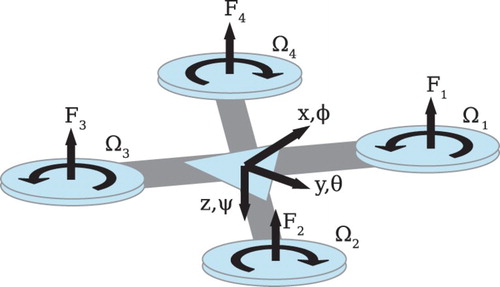
The vehicle is an underactuated system, so independently manipulating all six degrees of freedom is not possible. Forward and lateral translations are coupled to pitch and roll of the vehicle, so it must pitch to move longitudinally, and roll to move laterally. Rotation matrix R, described by

maps the body frame to the inertial frame, where sine and cosine (s_*, c_*) are applied to the vehicle attitude ().

2.2 Quadrotor dynamics

The vehicle is modeled as a rigid body with external forces and moments acting on the body. Gravity, the gyroscopic effects from the propellers, and the control inputs from the motors are the primary external forces and moments on the vehicle (Bouabdallah et al. 2004). This section presents the rigid body dynamics and then addresses external forces and moments individually.

Rigid body dynamics: The dynamics of a rigid body under external forces and moments expressed in the inertial frame are governed by

where and represent the external forces and moments acting on the vehicle, v is the velocity in the body frame, ω the angular rate of the vehicle, m the quadrotor mass, and J the moment of inertia matrix.

Control inputs: The controller design is better suited for manipulating forces and moments on the vehicle, but the vehicle is physically controlled by adjusting motor speeds. Simplified propeller dynamics reduce to a linear relationship between the squared rotor angular rate and the force and moment of the propellers. The relationship is given by

where i is the motor index, c_f and c_m are thrust and drag coefficients, and Ω_i the rotor angular velocity. The motors are all aligned with the vertical axis of the body frame, so the force and moments only occur in the z-direction of the body frame; i.e. F_xi=F_yi=0 and M_xi=M_yi=0, where F_z is negative to remain consistent with the downward z-axis convention. The relationship that maps motor angular velocities to forces and moments on the vehicle is

where d is the distance between the motors and CG.

Gyroscopic moment: The spinning propellers create a gyroscopic torque when the quadrotor rotates in space. All propellers have the same moment of inertia, so the sum of the rotor angular velocities, , can be used to model gyroscopic effects. The rotational velocity of the vehicle ω and the net angular velocity of the rotors Ω_r determine the resultant gyroscopic moment: .

Complete equations of motion: The complete equations of motion for the quadrotor are obtained by expanding out the rigid body dynamics, and then adding the external forces and moments from the control inputs, the gyroscopic effects, and the gravitational force. After manipulating terms, the vehicle dynamics are determined to be

which are expressed in the inertial frame. Sine and cosine terms (s_*, c_*) come from the rotation R between the body frame and the inertial frame, translation () is dictated by the vertical force from the props (F_z) and the attitude () of the quadrotor, and rotational acceleration () is dominated by the moments (M_x, M_y, M_z) from the props.

2.3 Linearized system

Linearization takes the nonlinear dynamic system, identifies meaningful operating points, and creates a linear model around those points. The nominal controller is developed around the linearized model, and the adaptive controller adapts to the linearized model during changing conditions.

The equations of motion of the plant are expressed in compact form as where

which has n=12 states and m=4 control inputs. Denote an operating point as ◯_p and û, so that perturbations are described by and . The Taylor series expansion of the nonlinear system yields

and after disregarding higher order terms (HOT), becomes

When an operating point is also an equilibrium point (derivatives are equal to zero), then and the system reduces to , where future equations omit the Δ symbol for readability.

Linearization is accurate within a small region, and most quadrotor controller research limits the flight envelop to stay within this trusted region. The proposed controller adapts to changes in the high-frequency gain matrix, K_p, so the vehicle can accommodate different and changing operating points during a flight.

General form: The general form of the linearized system uses arbitrary values for all the states. The state matrix A_p is filled with the partial derivatives with respect to each state

and the quadrotor's B_p matrix is populated with the partial derivatives with respect to each control input

where submatrices A_t, A_r, B_t, and B_r are given by

The controller uses diagonal matrices to decouple the inputs and outputs, so the system outputs must closely match the control inputs. With , the system output is selected as . Nominal control inputs are needed to complete the linearization process. Maintaining a zero rotational acceleration implies , whereas maintaining a zero vertical acceleration necessitates .

Hover condition: The logical starting point for linearization is around the hover condition. During hover the vehicle has zero tilt about the roll and pitch axes, the heading is arbitrary, and the angular rates must all be equal to zero. The position in space is arbitrary, but the velocities must all be zero. With this description, the nominal state is given by , and the nominal control input is given by . This state represents an equilibrium point, so . Evaluating A_p at the operating point yields

and evaluating B_p at the operating point yields

A similar procedure can be used to evaluate operating points other than the hover condition.

3. Control system design

This section addresses the conditions to implement the controller, describes the theory to develop a nominal controller for a multi-input multi-output (MIMO) system, and then builds upon that foundation to develop the adaptive controller for the quadrotor.

3.1 Plant assumptions

Consider a linearized MIMO system described by

with transfer matrix , where the parameters in A_p, B_p, and C are unknown. From Tao(2003a), we know that an m×m strictly proper and full rank rational transfer matrix G(s) has an interactor matrix ξ(s) such that the high-frequency gain matrix of G(s), defined as , is finite and nonsingular. Also, the high-frequency gain matrix , with all its leading principle minors Δ_i being nonzero, has a non-unique decomposition K_p=LDS, where S=S^T>0, is a unity lower triangular matrix, and

such that γ_i>0, i=1, … , m, is arbitrary.

For a MIMO state feedback controller, the following conditions must be satisfied (Tao 2003a):

• (1) (A_p, B_p) controllable and (A_p, C) observable;

• (2) all zeros of G(s) have negative real parts;

• (3) G(s) has full rank with known ξ(s); and

• (4) all leading principle minors Δ_i, i=1, … , m, of K_p are nonzero and their signs are known.

Condition (1) is needed for stable plant–model matching. Zeros of a MIMO system cause G(s) to lose rank, so that a control input u(t) ¬=0 exists where ; meaning the control input has no influence on the system output. Condition (2) ensures that no transmission zeros exist which can cause the system to become uncontrollable. Condition (3) is needed to select a viable reference model, and Condition (4) ensures that the adaptation laws converge in the correct direction.

3.2 Nominal controller design

All states are available for measurement, so state feedback control is used. This section describes state tracking control, and illustrates the limitations with the matching condition when plant matrices are unknown. Then output tracking is presented because it offers a simple control structure and alleviates the matching condition requirement.

State tracking: The goal of state feedback state tracking control is to influence the system (17), by designing a control input u(t) such that all the signals in the closed-loop system are bounded, and the state vector signal x_p(t) asymptotically tracks a reference state vector signal x_m(t). A bounded reference signal is applied to the reference system

where stable and describe the desired system characteristics. The control input

with and , achieves the desired control objective by producing a closed-loop system governed by . The gains must be selected so and B_m=B_p K_r, which describe the necessary matching condition (Franklin, Powell,& Emami-Naeini 2009).

Matching condition limitations: Consider the general structure of the quadrotor plant matrices A_p and B_p, given in Equations (9) and (10). Denote the submatrices as and for i, j=1, 2, 3, the column vector as , and the diagonal matrix as . The matching condition becomes

where

for i=1, 2, 3 and , and

for i=1, 2, 3 and j=1, 2, 3, 4. The sparse nature of the required A_m and B_m matrices, and the limited options for elements within those matrices, make the matching condition difficult or impossible to satisfy.

Output tracking: To alleviate the state tracking matching condition, an output tracking controller is presented. The goal of state feedback output tracking control is to influence the system (17), by designing a control input u(t) such that all the signals in the closed-loop system are bounded, and the output y_p(t) asymptotically tracks a reference output y_m(t); meaning . A bounded reference signal is applied to the reference system

where the closed-loop transfer matrix G_c is described by

and is the modified left interactor matrix, where d_i(s) are the desired closed-loop characteristic polynomials of degree l_i. The high-frequency gain matrix K_p is related to the control gains K_x and K_r through the relationships

where the i{th} row of K₀ is described by

where c_i is the ith row of the C matrix, and d_ij are coefficients of the desired characteristic polynomials (Goodwin,Graebe, & Salgado 2001).

Relaxed matching condition: Whereas, state tracking control requires a strict matching condition between and B_m=B_pK_r, the structure of the output tracking controller is more flexible. The gain matrices K_x and K_r are defined in terms of K₀, which encompasses the terms for the desired closed-loop characteristic polynomials d_i(s). These polynomials can be arbitrarily tailored to suit any desired system response. The only restriction on the selection of d_i(s) is the degree of each polynomial must match the degree of the plant interactor matrix ξ(s), which is common in any traditional pole placement controller design.

3.3 Adaptive controller design

When the state and input matrices A_p and B_p are known, the state feedback gains K_x and K_r can be uniquely determined (Chen 2013). However, when A_p and B_p are either unknown or changing, then static values for K_x and K_r are not appropriate. The uncertainty associated with the nominal controller motivates the development of the adaptive controller, where the parameters of A_p and B_p are estimated to determine the appropriate feedback gains.

The goal of the adaptive control algorithm is to have the system output y_p(t) track a desired output y_m(t) given by Equation (24), and to have the tracking error, , decay to zero exponentially. Let K_x* and K_r* denote the true (unknown) feedback gains, and K_x(t) and K_r(t) be their estimates. The feedback control law becomes

where K_x(t) and K_r(t) are updated from adaptive laws. Uncertainties in A_p and B_p are accounted for in the high-frequency gain matrix K_p, and the LDS decomposition of K_p is included within the adaptation process.

Control structure: Substituting the estimates of the gain matrices K_x(t) and K_r(t) for the control law yields

so the output tracking error is expressed as

where

When there is no estimation error, and . This indicates , because the estimation error is zero, and the stability of ensures converges to zero exponentially.

Error parametrization: Following Guo et al. (2011), we ignore the exponentially decaying term, and substitute the LDS decomposition for K_p, so the tracking error is expressed as

Eliminate the unity on the diagonal in L⁻¹ by introducing , so that on its diagonal and upper triangle, and then substituting in Λ* yields

Introduce a stable filter F(s)=1/f(s), where f(s) is a stable monic polynomial, where the degree of f(s) matches the degree of ξ_m(s). Operate on both sides by F(s), so

where the transformed error signal is given by

The term can be expressed as

where and , for i=2, … , m, and isolate the transformed error so

Let be the estimate of , and denoting Ψ*=DS, let Ψ(t) be the estimate of Ψ*. Estimation errors are the difference between the estimates and their true values, so

Define ε(t) as the summation of all the parameter estimates

where and . Substituting in the transformed tracking error yields

which puts ε(t) completely in terms of parameter errors.

Adaptive laws: The estimates do not always equal their true values, so K_x(t) and K_r(t) are updated from adaptive laws. Select a normalizing signal m(t) described by

then the expression for the estimation error ε(t) suggests the following adaptive laws:

where the adaptive gains are selected so that and , for i=2, 3, … , m.

Stability analysis: To evaluate the closed-loop stability, define a positive definite function as

and calculate its time derivative as

Having implies that all the estimation signals are bounded: , , and for i=2, … , m. It also shows that , which implies that , , and for i=2, … , m. From these properties, the boundedness of x_p(t) can be shown. The boundedness of x_p(t), r(t), K_x(t), and K_r(t) guarantees that u(t) is bounded, thus all closed-loop control signals are bounded and approaches zero asymptotically (Hsu, Costa, Imai, and Kokotovic 2001).

4. Quadrotor controller development

This section utilizes established control theory to develop the nominal controller, and then expands to the adaptive control architecture applied to the quadrotor system.

4.1 Quadrotor nominal controller

Before embarking on the adaptive controller analysis, it is crucial to understand the characteristics of the vehicle and the structure of the nominal controller. To numerically evaluate the system, consider a quadrotor with the following estimated parameters: , m=0.6 kg, , , , and , with dimensions n=12 and m=4. The system is a special form where the number of inputs equals the number of outputs. For the nominal controller, the parameter estimates are assumed to be the true values which are used to determine K_x* and K_r*.

Using the specified parameters and inserting zeros for all the states yields the following state and input submatrices:

where the system transfer matrix G(s) is described by

where d(s)=s⁴ is the characteristic equation after pole/zero cancelations. The controllability and observability matrices are both full rank, so the system is fully controllable and observable; and the system transfer matrix G(s) is full rank and strictly proper, which satisfies the design condition.

Finding the poles and zeros of a MIMO system is accomplished with the Smith-McMillan form, described by Goodwin et al. (2001) and Hosoe (1975). Find the greatest common divisors χ_i(s) of all i×i minor determinants of N(s). Then forms , which is used to find the diagonal elements of the Smith-McMillan matrix. Following the procedure, the Smith-McMillan form becomes

where the system zeros are calculated as

and the system poles are found to be

so there are no zeros and 12 poles located at the origin.

The interactor matrix of the quadrotor is generally diagonal, and forms the high-frequency gain matrix

which must be finite and nonsingular; so the limit of all elements of K_p must not grow to infinity, and the determinant must be nonzero. Selecting l₂=l₃=4 and l₁=l₄=2 yields , and the high-frequency gain matrix becomes

where . The polynomials d_i(s) in the modified interactor matrix ξ_m(s) must have degrees of l_i, and the desired poles can be placed arbitrarily. For this analysis, all poles are located at −2, which gives the following:

and

The coefficients d_ij from the polynomials

are used to populate the K₀ matrix which determines the K_x* and K_r* matrices. After pole/zero cancelations, the closed-loop system is described by G_c(s), given as

which shows that the transfer matrix fits the desired form, and all of the poles have been successfully placed at s=−2.

4.2 Quadrotor adaptive controller

When implementing the adaptive controller, the initial parameter estimates are not expected to equal their true values. However, the controller needs to be initialized with some starting values. The initial guesses for the parameters can be used to determine appropriate starting points.

From the nominal controller development, use the initial parameter guesses to find K_x(0) and K_r(0), which provides a starting point to populate Θ(0). In a similar way, the initial parameter estimates form an approximate value for the high-frequency gain matrix, denoted as Kˆ_p. Because the other two parameter estimates, Ψ(t) and , are based on the LDS decomposition of K_p, we can also determine suitable starting values for those matrices.

The structure of D(t) is known to be diagonal, with our choice of γ_i. For simplicity, select S(0)=I₄ as a starting point. Ideally, the parameter estimates should be initialized with zero values, and then adapt as needed. Setting L(0)=I₄ achieves , so selecting values for γ_i is all that remains. The relationship is

where

indicate that D(0) should be initialized with Kˆ_p, so the gain is set to .

5. Simulation study

Two simulations are presented as part of this research. The first simulation shows the system response to a step change in altitude which is then subjected to a physical disturbance. The second simulation illustrates the vehicle trajectory while following a circular path with an initial position error. When running the adaptive controller simulations, the true parameter values are set so that the mass and the moment of inertias are 110% of their estimated values. Both simulations use the parameter and gain values developed previously.

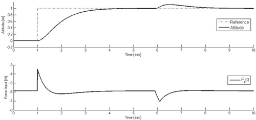
Elevation change: The quadrotor is initially at rest at the origin. At 1.0 s, the reference signal increases altitude by 1.0 m, and at 6.0 s, the system is disturbed by a 2.0 N force. The controller development arbitrarily sets the poles at −2, which implies the system is overdamped. The elevation change simulation, provided in Figure 2, confirms the system is overdamped, because there is no overshoot and the response has a rise time around 2.5 s. The poles of the characteristic polynomials were arbitrarily selected, so the design can be adjusted to achieve a custom system response. The simulation also confirms that the disturbance is quickly rejected, where the system returns to the reference altitude within 2.0 s.

Figure 2. Elevation change: altitude and force input.

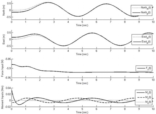
Circular path: The quadrotor starts at rest with an initial position error of 0.15 m in both the north and east directions. The reference signal trajectory is defined as a loiter where the vehicle circles around the origin following a 0.5 m radius at 4.0 s per cycle. The simulation results are provided in Figure 3, which illustrates the quadrotor is capable of tracking the prescribed reference output. Whereas, a fixed controller will have a steady-state error with a sinusoidal signal, the tracking error with the adaptive controller decays to zero exponentially. For this simulation, the tracking error is eliminated within 3.0 s.

Figure 3. Circular path: north/east positions and force/moment inputs.

Simulation summary: The two simulations illustrate important characteristics of the adaptive control system. The control system for both simulations uses arbitrarily prescribed characteristics, so the controller can be further adjusted to achieve any particular system response. The first case shows that the quadrotor accurately tracks a given reference signal, and the vehicle adequately rejects disturbances. The second simulation is more complex with two states changing over time. Despite the coupling between inputs and outputs, the system still tracks the reference signal. The controller successfully rejected the initial position error, and the steady-state error decayed to zero exponentially.

6. Conclusions

This research developed the dynamics, equations of motion, and linearization for the quadrotor vehicle which laid the groundwork for the controller development. Existing linear control theory for both fixed and adaptive controllers was reviewed and applied to the quadrotor system. The adaptive controller was based on an LDS decomposition which relaxed the matching condition between the plant and model structure. This approach maintained the simple state feedback controller structure, and avoided the more complicated output feedback structure. Using this decomposition placed the uncertainty of the high-frequency gain matrix K_p within the adaptation process, which allows the controller to adapt to both parameter uncertainty and varying operating points. It was demonstrated that the adaptive control system ensures closed-loop stability and asymptotic output tracking; and a simulation analysis showed that the quadrotor can overcome initial errors, track reference signals, and reject disturbances, despite coupling between states. Expanding the range of operating points for quadrotor UAVs increases their robustness, which may increase their number of applications.

REFERENCES

- Bouabdallah, S., Murrieri, P., & Siegwart, R. (2004, April). Design and control of an indoor micro quadrotor. Proc. of the 2004 IEEE international conference on robotics and auto, New Orleans, LA, pp. 4393–4398.
- Chen, C. (2013). Linear system theory and design. New York: Oxford University Press.
- Das, A., Subbarao, K., & Lewis, F. (2009). Dynamic inversion with zero-dynamics stabilization for quadrotor control. IET Control Theory and Applications, 3(3), 303–314. doi: 10.1049/iet-cta:20080002
- Diao, C., Xian, B., Yin, Q., Zeng, W., Li, H., & Yang, Y. (2011, May). A nonlinear adaptive control approach for quadrotor UAVs. Proc. of the 2011 8th Asian control conference, Kaohsiung, Taiwan.
- Dydek, Z., Annaswamy, A., & Lavretsky, E. (2013). Adaptive control of quadrotor UAVs: A design trade study with flight evaluations. IEEE Transactions on Control Systems Technology, 21(4), 1400–1406. doi: 10.1109/TCST.2012.2200104
- Elliott, H., & Wolovich, W. (1982). A parameter adaptive control structure for linear multivariable systems. IEEE Transactions on Automatic Control, 27(2), 340–352. doi: 10.1109/TAC.1982.1102914
- Franklin, G., Powell, J., & Emami-Naeini, A. (2009). Feedback control of dynamic systems. Upper Saddle River, NJ: Pearson.
- Goodwin, G., Graebe, S., & Salgado, M. (2001). Control system design. Upper Saddle River, NJ: Prentice Hall.
- Goodwin, G., & Sin, K. S. (1984). Adaptive filtering prediction and control. Englewood Cliffs, NJ: Prentice Hall.
- Guo, J., Liu, Y., & Tao, G. (2009). Multivariable MRAC with state feedback for output tracking. Proc. of the 2009 ACC, St. Louis, MO, USA. pp. 592–597.
- Guo, J., Tao, G., & Liu, Y. (2011, April). A multivariable MRAC scheme with application to a nonlinear aircraft model. Automatica, 47, 804–812. doi: 10.1016/j.automatica.2011.01.069
- Hehn, M., & D'Andrea, R. (2011, May). A flying inverted pendulum. IEEE international conference on robotics and automation, Shanghai, China. pp. 763–770.
- Hosoe, S. (1975, December). On a time-domain characterization of the numerator polynomials of the Smith-McMillan form. IEEE Transactions on Automatic Control, 20(6), pp. 799–800. doi: 10.1109/TAC.1975.1101097
- Hsu, L., Costa, R.R., Imai, A.K., & Kokotovic, P. (2001). Lyapunov-based adaptive control of MIMO systems. Proc. of the 2001 ACC, Arlington, VA, USA, pp. 4808–4813.
- Imai, A.K., Costa, R.R., Hsu, L., Tao, G., & Kokotovic, P. (2001, December). Multivariable MRAC using high-frequency gain matrix factorization. Proc. of the 40th IEEE conference on decision and control, Orlando, FL, pp. 1193–1198.
- Ioannou, P., & Sun, J. (1996). Robust adaptive control. Upper Saddle River, NJ: Prentice Hall.
- Isidori, A. (1995). Nonlinear control systems. Berlin: Springer-Verlag.
- Krstic, M., Kanellakopoulos, I., & Kokotovic, P. V. (1995). Nonlinear and adaptive control design. New York: John Wiley & Sons.
- Madani, T., & Benallegue, A. (2006, October). Backstepping control for a quadrotor helicopter. Proc. of the 2006 IEEE/RSJ, international conference on intelligent robots and systems, Beijing, China, pp. 3255–3260.
- Nicol, C., Macnab, C. J. B., & Ramirez-Serrano, A. (2011). Robust adaptive control of a quadrotor helicopter. Mechatronics, 21, 927–938. doi: 10.1016/j.mechatronics.2011.02.007
- Pounds, P., Mahony, R., & Corke, P. (2010). Modelling and control of a large quadrotor robot. Control Engineering Practice, 18, 691–699. doi: 10.1016/j.conengprac.2010.02.008
- Tao, G. (2003a). Adaptive control design and analysis. Hoboken, NJ: John Wiley and Sons.
- Tao, G. (2003b). A unification of multivariable MRAC based on high-frequency gain matrix decompositions. Proc. of the 2003 ACC, Denver, CO, USA, pp. 945–950.