Design of a robust tracking controller for a nonholonomic mobile robot with side slipping based on Lyapunov Redesign and nonlinear H_∞ methods

ABSTRACT

In this paper, robust control of nonholonomic mobile robots is considered which is more complex with respect to holonomic types, due to fewer degrees of freedom in their model. In addition, side slipping is considered which disturbs the nonholonomic constraint adversely. In previous researches, the slip is either estimated by an estimator or is measured using additional sensors. In this paper, the Kanayama transformation is modified such that the model of the robot only includes matched disturbances. Then, a robust tracking controller is designed using the Lyapunov redesign method when only the upper bound of the side slip is known. Moreover, in order to compare the performance of the proposed controller, the nonlinear H_∞ control is also developed for this robot. Finally, the performance of these two controllers is compared and the simulation results show the appropriate efficiency of the proposed controllers.

KEYWORDS:

• Nonholonomic
• slipping
• Kanayama
• Lyapunov Redesign method
• nonlinear H_∞ method

1. Introduction

Mobile Robots are applicable in different industries such as transmission of materials, military and oil industries. One important category of mobile robots includes nonholonomic ones with nonintegrable constraints. In this category, nonholonomic constraints are due to the assumption that the robot could not move side-wise. However, the slipping can violate the nonholonomic constraints, adversely. Therefore, one important issue is to design a robust controller for nonholonomic mobile robots to compensate the effects of slipping.

In general, dynamic equations of nonholonomic mobile robots are such that in most studies, the backstepping technique is used in the design process (Pourboghrat & Karlsson, 2002). The basic of this technique is to control the linear and angular velocities of the robot, using the input torques and, then tracking the desired path using the controlled velocities. Therefore, in the first step, the linear and angular velocities of the robot are assumed as control variables, to converge the tracking errors to zero. This step is called virtual control. Then, the input torques are designed to converge the mentioned velocities to their desired values.

Many researchers have proposed tracking controllers for a nonholonomic mobile robot (without slipping), using several nonlinear control methods. For instance, in (Pourboghrat & Karlsson, 2002; JIANGdagger & Nijmeijer, 1997; Fierro & Lewis, 1995; Do, 2013), tracking controllers for this robot using backstepping structure and the Lyapunov based methods have been proposed. In (Yang & Kim, 1999; Binazadeh & Shafiei, 2014a; Chwa, 2004), tracking controllers are designed for a nonholonomic mobile robot, using the sliding mode control method in polar coordinates with bounded external disturbances. Moreover, in (Miyasato, 2008), using nonlinear $H_{\mathrm{\infty }}$ control, an adaptive tracking controller has been designed for a robot with uncertainties in the mass, moment of inertia and friction constants of the wheels. Also, in (Li et al., 2010), a control algorithm based on backstepping and sliding mode techniques to control a nonholonomic mobile robot has been proposed.

Unfortunately, these researches have not been developed for the slipping case. In the case of slipping robots, in (Zhou et al., 2007), a tracking controller using the backstepping technique and Lyapunov analysis has been designed in which the slip is estimated by an unscented Kalman filter. In (Yoo, 2013; Li et al., 2018), according to the estimation of slip value and the model’s uncertainties, a controller has been designed by a neural network to track a desired trajectory. Moreover, in (Du et al., 2015), an observer to estimate the side-slip angle has been designed and an observer-based controller for a vehicle with considering the side-slip has been proposed. In the estimation-based methods, a dynamical model is added to the closed-loop system and this leads to a higher-order system which is complicated for closed-loop analyses. Moreover, estimation-based algorithms depend on the model of the system and generally, model-based methods are not robust. On the other hand, in the references like (Li et al., 2018), the slip value has been measured by a GPS receiver and a number of auxiliary sensors. However, using additional sensors make the robot expensive. In (Taheri-Kalani and Khosrowjerdi, 2014; Hwang et al., 2013), adaptive tracking controllers with considering slip have been proposed. The considered slip in (Taheri-Kalani and Khosrowjerdi, 2014) is estimated by a disturbance observer. Whereas, in (Hwang et al., 2013) a robust tracking controller using backstepping technique and Lyapunov redesign method in the presence of slipping, has been proposed. However, in the model considered in (Zhou et al., 2007; Yoo, 2013; Li et al., 2018; Du et al., 2015; Taheri-Kalani and Khosrowjerdi, 2014; Hwang et al., 2013), the admissible amount of the slip value is too small and it only deviates the robot position from its main path. Whereas, the slip value may deviate the direction of the velocity vector (rotating the robot around itself).

In this paper, a tracking controller is suggested for a nonholonomic mobile robot which is robust to the effects of the side slip. In the proposed controller, it is not necessary to have a sensor to measure the value of side slip or an estimator to estimate it. In fact, the priori knowledge in the design procedure includes only an upper bound of the possible slip values. Moreover, the model used in this paper is a more perfect model with respect to the references which have controlled such a robot in the presence of the side slip.

The structure of this paper is as follows; in Section 1, the model of a nonholonomic mobile robot with considering the side slip will be introduced. In Section 2, the tracking problem for the robot will be described. A tracking robust controller will be designed based on Lyapunov redesign method in Section 3. Also, in Section 4, in order to compare the performance of the proposed controller, the nonlinear $H_{\mathrm{\infty }}$ method will be developed in the case of the robot with side slip. Finally, simulation results and comparison of two controllers will be presented for a robot with real values.

2. Model of a nonholonomic mobile robot in the presence of side slip

Figure 1, shows the configuration of a robot in the presence of side-slip. In this robot, the torque inputs are applied to the rear wheels and the front wheel is a castor. The body reference frame of this robot includes axis coordinates of $X_b$ and $Y_b$ and the reference point $P$ (centre of mass) which forms the angle of $\varphi$ with the inertial reference frame, $X$ and $Y$. The vector $\overrightarrow{v}$ is the velocity of the reference point $P$ and ${\overrightarrow{v}}_y$ and ${\overrightarrow{v}}_l$ are the components of $\overrightarrow{v}$ along the $Y_b$ and $X_b$ axes, respectively. Also, the velocity reference frame of this robot includes axis coordinates of $X_v$ and $Y_v$.

Figure 1. Configuration of a nonholonomic mobile robot in the presence of the side slip.

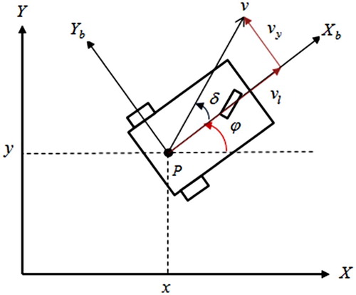
The velocities ${\overrightarrow{v}}_y$ and ${\overrightarrow{v}}_l$, are related to the slip angle ($\delta$), as follows (Wang and Low, 2008): (1) $\begin{array}{rl}\sin \delta & =\frac{v_y}{v}\\ \cos \delta & =\frac{v_l}{v}\end{array}$(1) Therefore, the kinematic model of a nonholonomic mobile robot in the presence of side slip is as follows: (2) $\begin{array}{rl}\dot{x}& =v\cos (\varphi +\delta )\\ \dot{y}& =v\sin (\varphi +\delta )\\ \dot{\varphi }& =\omega +\sigma \end{array}$(2) where $v$ and $\omega$ are the linear and angular velocities of the robot, respectively. In this model, the variable, $\sigma$ is the effect of slip on the direction of the velocity vector. In other words, the slip in addition to deviating the robot position from its main path, also, rotates the main axis of the robot.

In the kinematic model of the nonholonomic mobile robot, the torque inputs, ${\tau }_1,{\tau }_2$ which are applied to the rear wheels have not appeared. Therefore, regarding to Newton laws, it is found that (3) $\begin{array}{rl}\dot{v}& =\frac{1}{rm}({\tau }_1+{\tau }_2)=b_1{u}_1\\ \dot{\omega }& =\frac{l}{rI}({\tau }_2-{\tau }_1)=b_2{u}_2\end{array}$(3) where $b_1=\frac{1}{rm}$ and $b_2=\frac{l}{rI}$. The parameters $m$ and $I$ are the mass and moment of inertia of the robot, respectively. Also, $u_1={\tau }_1+{\tau }_2$ and $u_2={\tau }_1-{\tau }_2$ are the control signals of the system. Using Equations (2) and (3), the dynamical model of the nonholonomic mobile robot will be achieved as (4) $\begin{array}{rl}\ddot{x}& =b_1{u}_1\cos (\varphi +\delta )+\frac{\lambda }{m}\sin (\varphi +\delta )\\ \ddot{y}& =b_1{u}_1\sin (\varphi +\delta )-\frac{\lambda }{m}\cos (\varphi +\delta )\\ \ddot{\varphi }& =\dot{\omega }+\dot{\sigma }\end{array}$(4) where $\lambda$ is the Lagrange coefficient and is defined as (5) $\lambda =-m(\dot{\varphi }+\dot{\delta })\left[\dot{x}\cos (\varphi +\delta )+\dot{y}\sin (\varphi +\delta )\right]$(5)

3. Statement of the tracking problem

In tracking problems, it is necessary to define the tracking error and to develop the error dynamical equations. The tracking problem includes a reference trajectory $q_r\left(t\right)=[x_r\left(t\right),y_r\left(t\right),{\varphi }_r\left(t\right){]}^T$ which should be followed by the considered robot, i.e. the robot trajectory $q\left(t\right)=[x\left(t\right),y\left(t\right),\varphi \left(t\right){]}^T$ must be consistent with $q_r\left(t\right)$. The reference trajectory $q_r\left(t\right)$ is created by a reference robot in order to satisfy the equations of a kinematic model of the mobile robot and nonholonomic constraints. Thus, to generate $q_r\left(t\right)$, the desired values of linear and angular velocities are applied as input signals to the kinematic equation of an ideal robot (Equation (6)). The state variables of this ideal robot is the reference trajectory which should be tracked. The kinematic equations of the reference robot are as follow: (6) $\begin{array}{rl}{\dot{x}}_r& =v_r\cos {\varphi }_r\\ {\dot{y}}_r& =v_r\sin \varphi {}_r\\ {\dot{\varphi }}_r& ={\omega }_r\end{array}$(6) where the subscript $r$ stands for reference trajectory variables, and $v_r$, ${\omega }_r$ are the desired values of linear and angular velocities of the reference robot, respectively (Pourboghrat and Karlsson, 2002).

The following assumptions have been commonly used in the papers which have designed a tracking controller based on the Lyapunov theorem (Pourboghrat and Karlsson, 2002; JIANGdagger and Nijmeijer, 1997; Fierro and Lewis, 1995; Wang and Tsai, 2005; Kanayama et al., 1990):

Assumption 1: Linear and angular velocities of the reference robot and their first derivatives are assumed to be available and bounded.

Assumption 2: In the tracking problem, it is assumed that the linear and angular velocities of the reference robot do not go to zero, simultaneously.

The goal of tracking is to find a feedback control law as $(u_1,u_2{)}^T=u(q,\dot{q},q_r,v_r,{\omega }_r,{\dot{v}}_r,{\dot{\omega }}_r)$ such that with considering the side slip, the value of $\tilde{q}\left(t\right)=q_r\left(t\right)-q\left(t\right)$ (the difference between the reference and real trajectories) converges to zero. In order to make the tracking errors independent from the inertial reference frame, the Kanayama transformation is applied to the vector $\tilde{q}\left(t\right)$ (Do, 2013). This transformation is a conversion in the form of a rotation with the value of $\varphi$ which transfers the inertial reference frame into the body reference frame. However, in this paper due to the presence of the slip, the rotation angle of $(\varphi +\delta )$ instead of $\varphi$ is proposed which transfers the inertial reference frame into the velocity reference frame. Moreover, in the vector $\tilde{q}\left(t\right)$, the third component (the angle error) is replaced by ${\varphi }_e={\varphi }_r-(\varphi +\delta )$. This means that (7) $\left(\begin{array}{c}{e}_1\\ e_2\\ e_3\end{array}\right)=\left(\begin{array}{ccc}\cos (\varphi +\delta )& \sin (\varphi +\delta )& 0\\ -\sin (\varphi +\delta )& \cos (\varphi +\delta )& 0\\ 0& 0& 1\end{array}\right)\left(\begin{array}{c}{x}_r-x\\ y_r-y\\ {\varphi }_r-(\varphi +\delta )\end{array}\right)$(7) where $e=(e_1,e_2,e_3{)}^T$ is the vector of tracking errors in the velocity reference frame and the matrix $T$ is the rotation matrix. This transformation leads to have a model which includes only matched disturbances in order to apply the Lyapunov redesign and nonlinear $H_{\mathrm{\infty }}$ methods. Therefore, dynamical equations of the vector of tracking errors with considering the side slip can be described as follow: (8) $\begin{array}{rl}{\dot{e}}_1& =e_2(\omega +\sigma +\dot{\delta })-v+v_r\cos e_3\\ {\dot{e}}_2& =-e_1(\omega +\sigma +\dot{\delta })+v_r\sin e_3\\ {\dot{e}}_3& ={\omega }_r-\omega -\sigma -\dot{\delta }\end{array}$(8)

4. Design of a robust tracking controller based on Lyapunov Redesign

The objective of this section is to design a robust tracking controller using the backstepping and Lyapunov Redesign methods such that the vector of tracking errors $e$ in the presence of side slip converges to zero, asymptotically. In the proposed method, first, a nominal controller without considering the slip will be designed. Then, the tracking in the presence of side slip will be achieved using Lyapunov Redesign method.

4.1. Nominal Controller design

Since, the real inputs of the system, $u_1$ and $u_2$, have not appeared in Equation (8), the variables $v$ and $\omega$ are considered as virtual controller inputs for this system. These virtual inputs are designed based on Lyapunov theorem to asymptotically stabilize the system (8). The dynamical equations of errors, without side slip (nominal system), are described as follow: (9) $\begin{array}{rl}{\dot{e}}_1& =e_2\omega -v+v_r\cos e_3\\ {\dot{e}}_2& =-e_1\omega +v_r\sin e_3\\ {\dot{e}}_3& ={\omega }_r-\omega \end{array}$(9) The following theorem proposes a stabilizing controller for the system (9):

Theorem 4.1:

Consider the system (9) with the following virtual control laws: (10) $\begin{array}{rl}v& =k_1{e}_1+v_r\cos e_3\\ \omega & ={\omega }_r+k_2{e}_2{v}_r+k_3\sin e_3\end{array}$(10) where $k_1$, $k_2$ and $k_3$ are arbitrary positive constants. Then, the closed-loop system is asymptotically stable and the tracking errors converge to zero.

Proof:

Using the proposed control laws (10) and the equations of the nominal system (9), the equations of the closed-loop system are as follow: (11) $\begin{array}{rl}{\dot{e}}_1& =e_2({\omega }_r+k_2{e}_2{v}_r+k_3\sin e_3)-k_1{e}_1\\ {\dot{e}}_2& =-e_1({\omega }_r+k_2{e}_2{v}_r+k_3\sin e_3)+v_r\sin e_3\\ {\dot{e}}_3& =-k_2{e}_2{v}_r-k_3\sin e_3\end{array}$(11) It can be easily shown that the closed-loop system (11) has two equilibrium points as $(e_1,e_2,e_3{)}^T=(0,0,0{)}^T$, $(e_1,e_2,e_3{)}^T=(0,0,\pi {)}^T$. It is shown that the first point (origin) is a stable equilibrium point and the second one is unstable.

To prove the stability of the origin, a positive definite Lyapunov function is selected as follows: (12) $V_1=\frac{1}{2}(e_1^2+e_2^2)+\frac{1}{k_2}(1-\cos e_3)$(12) where $k_2$ is a positive constant. Then, the derivative of the Lyapunov function along the system (9) results in (13) ${\dot{V}}_1=-k_1{e}_1^2-\frac{k_3}{k_2}{\sin }^2{e}_3\le 0$(13) Although the function ${\dot{V}}_1$ is negative semi-definite, it is proved that the system (11) is asymptotically stable using Barbalat’s lemma (Slotine and Li, 1991). Since, $V_1$ is bounded from below (it is a positive definite function) and ${\dot{V}}_1\le 0$ (negative semi-definite), then $V_1$ will be bounded. Also, according to (12), boundedness of $V_1$ leads to have the variables $e_1$ and $e_2$ with bounded values. In addition, using equations (11) and (12), the second derivative of $V_1$ is as (14) $\begin{array}{rl}{\ddot{V}}_1& =-2k_1{e}_1{e}_2({\omega }_r+k_2{e}_2{v}_r+k_3\sin e_3)+2k_1^2{e}_1^2\\ & +\frac{2k_3}{k_2}\sin e_3\cos e_3(k_2{e}_2{v}_r+k_3\sin e_3)\end{array}$(14) Since, the constants $k_1$, $k_2$ and $k_3$ are bounded and considering Assumption 1, ${\ddot{V}}_1$ is bounded too. This means that ${\dot{V}}_1$ is uniformly continuous. Therefore, according to the Barbalat’s lemma, ${\dot{V}}_1$ converges to zero, as time approaches to infinity. Consequently, $e_1$ and $\sin e_3$ will converge to zero too.

To show that $e_2$ will also converges to zero, consider the following dynamical equation of $e_1$ in the system (11) which is rewritten here (15) ${\dot{e}}_1=e_2{\omega }_r+e_2(k_2{e}_2{v}_r+k_3\sin e_3)-k_1{e}_1$(15) Similar to the previous discussion, it can be easily shown that the second derivative of e₁ is bounded and again according to the Barbalat’s lemma, ${\dot{e}}_1$ converges to zero, as $t\to \mathrm{\infty }$. Therefore, Equation (15) leads to the following equation: (16) $e_2{\omega }_r+k_2{e}_2^2{v}_r=0$(16) Similarly, consider the dynamical equation of $e_3$ in system (11) which is rewritten here (17) ${\dot{e}}_3=-k_2{e}_2{v}_r-k_3\sin e_3$(17) The second derivative of $e_3$ is bounded too and according to the Barbalat’s lemma ${\dot{e}}_3$ converges to zero, as $t\to \mathrm{\infty }$. Therefore, Equation (17) simplifies to (18) $k_2{e}_2{v}_r=0$(18) According to Assumption 2 and Equations (16), (18), $e_2$ converges to zero. It means that the asymptotic stability of the origin in system (11) is guaranteed.

As mentioned before, there is another equilibrium point in system (11). To prove that the second equilibrium point is unstable, Chetaev instability theorem (Khalil, 2002) will be used. First, this point will be shifted to the origin with the conversion, ${\overline{e}}_3=e_3-\pi$. Therefore, the state space equation of the closed-loop system (11) with this conversion is as follows: (19) $\begin{array}{rl}{\dot{e}}_1& =e_2({\omega }_r+k_2{e}_2{v}_r-k_3\sin {\overline{e}}_3)-k_1{e}_1\\ {\dot{e}}_2& =-e_1({\omega }_r+k_2{e}_2{v}_r-k_3\sin {\overline{e}}_3)-v_r\sin {\overline{e}}_3\\ {\dot{\overline{e}}}_3& =-k_2{e}_2{v}_r+k_3\sin {\overline{e}}_3\end{array}$(19) Now, the origin of this system which is equivalent to the second equilibrium point in system (11) is analysed. In the Chetaev instability theorem, it is not necessary to use a positive definite function and the chosen function should be positive in one x₀ which is close enough to the origin. Therefore, the following function is selected: (20) ${\overline{V}}_1=-\frac{1}{2}(e_1^2+e_2^2)+\frac{1}{k_2}(1-\cos {\overline{e}}_3)$(20) This function is zero (at the origin) and it is positive in the region which is shown in Figure 2.

Figure 2. The subspace of $R^3$, where the function ${\overline{V}}_1$ is positive.

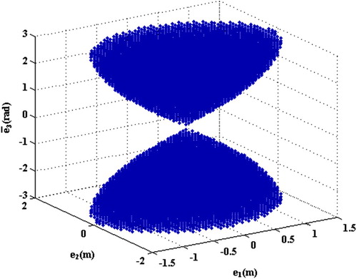
The derivative of this Lyapunov function for the closed-loop system (19) is as follows: (21) ${\dot{\overline{V}}}_1=k_1{e}_1^2+\frac{k_3}{k_2}{\sin }^2{\overline{e}}_3>0$(21) Since, in the region which has been shown in Figure 2, ${\overline{V}}_1$ and ${\dot{\overline{V}}}_1$ are positive, according to the instability theorem, the second point is unstable and the robot will not converge to this point.

4.2. Design of a robust virtual tracking controller using the Lyapunov Redesign method

In this section, a robust tracking controller will be designed based on the Lyapunov Redesign method.

Theorem 4.2:

Consider the system (8) with the following robust virtual control laws: (22) $\begin{array}{rl}v& =k_1{e}_1+v_r\cos e_3\\ \omega & ={\omega }_r+k_2{e}_2{v}_r+k_3\sin e_3+\eta \mathrm{sgn}\left(\sin e_3\right)\end{array}$(22) Then, the closed-loop system is asymptotically stable and the tracking errors converge to zero.

Proof: Considering Equations (8) and (22), the closed-loop system in the presence of side slip is as follows: (23) $\begin{array}{rl}{\dot{e}}_1& =e_2({\omega }_r+k_2{e}_2{v}_r+k_3\sin e_3+\eta \mathrm{sgn}(\sin e_3)+\sigma +\dot{\delta })\\ & -k_1{e}_1\\ {\dot{e}}_2& =-e_1({\omega }_r+k_2{e}_2{v}_r+k_3\sin e_3+\eta \mathrm{sgn}(\sin e_3)\\ & +\sigma +\dot{\delta })+v_r\sin e_3\\ {\dot{e}}_3& =-k_2{e}_2{v}_r-k_3\sin e_3-\eta \mathrm{sgn}\left(\sin e_3\right)-\sigma -\dot{\delta }\end{array}$(23) If the Lyapunov function (12) is considered, ${\dot{V}}_1$ along the system (23), will be as follows: (24) $\begin{array}{rl}{\dot{V}}_1& =-k_1{e}_1^2-\frac{k_3}{k_2}{\sin }^2{e}_3\\ & -\frac{1}{k_2}\sin e_3\left(\eta \mathrm{sgn}\left(\sin e_3\right)+\sigma +\dot{\delta }\right)\end{array}$(24) According to the inequality (13) one has (25) ${\dot{V}}_1\le -\frac{\eta }{k_2}\sin e_3\mathrm{sgn}\left(\sin e_3\right)-\frac{1}{k_2}\sin e_3(\sigma +\dot{\delta })$(25) On the other hand, to satisfy inequality (25), it is necessary to assume an upper bound on the slip value. If $||\sigma \left(t\right)+\dot{\delta }\left(t\right)|{|}_{\mathrm{\infty }}\le \beta$ one has (26) ${\dot{V}}_1\le -\frac{1}{k_2}|\sin e_3|(\eta -\beta )$(26) If $\eta \ge \beta$, according to the Barbalat’s lemma, the asymptotic stability of the closed-loop system (23) in the presence of side slip will be achieved.

4.3. The Real tracking controller design

The designed control laws (22) are not realistic and $v$, $\omega$ are not real inputs of the robot. Since the robot is controlled using the torques ${\tau }_1$ and ${\tau }_2$, the control laws (22) are considered as desired values of linear and angular velocities ($v_d,{\omega }_d$). Therefore, it is essential to design another controller to converge the linear and angular velocities of the robot to $v_d$ and ${\omega }_d$. In fact, in the transient response of the system, the desired and real velocities may not be the same. Therefore, two new state variables are defined as follow: (27) $\begin{array}{rl}\tilde{v}& =v-v_d\\ \tilde{\omega }& =\omega -{\omega }_d\end{array}$(27) Then, according to these new definitions and the dynamical Equations (3) and (8) one has (28) $\begin{array}{rl}{\dot{e}}_1& =e_2({\omega }_d+\tilde{\omega }+\sigma +\dot{\delta })-v_d-\tilde{v}+v_r\cos e_3\\ {\dot{e}}_2& =-e_1({\omega }_d+\tilde{\omega }+\sigma +\dot{\delta })+v_r\sin e_3\\ {\dot{e}}_3& ={\omega }_r-{\omega }_d-\tilde{\omega }-\sigma -\dot{\delta }\\ \dot{\tilde{v}}& =b_1{u}_1-{\dot{v}}_d\\ \dot{\tilde{\omega }}& =b_2{u}_2-{\dot{\omega }}_d\end{array}$(28)

Theorem 4.3:

Consider the system (28) with the following real control laws: (29) $\begin{array}{rl}{u}_1& =\frac{1}{b_1}(-c_1\tilde{v}+e_1+{\dot{v}}_d)\\ u_2& =\frac{1}{b_2}(-c_2\tilde{\omega }+\frac{\sin e_3}{k_2}+{\dot{\omega }}_d)\end{array}$(29) where $c_1$ and $c_2$ are arbitrary positive constants. Then, the closed-loop system is asymptotically stable and the tracking errors and also $\tilde{v}$ $\tilde{\omega }$ converge to zero.

Proof:

Using the proposed control laws of Equations (22) and (29) the closed-loop system is as follow: (30) $\begin{array}{rl}{\dot{e}}_1& =e_2({\omega }_r+k_2{e}_2{v}_r+k_3\sin e_3+\eta \mathrm{sgn}(\sin e_3)\\ & +\tilde{\omega }+\sigma +\dot{\delta })-k_1{e}_1-\tilde{v}\\ {\dot{e}}_2& =-e_1({\omega }_r+k_2{e}_2{v}_r+k_3\sin e_3+\eta \mathrm{sgn}(\sin e_3)\\ & +\tilde{\omega }+\sigma +\dot{\delta })+v_r\sin e_3\\ {\dot{e}}_3& =-k_2{e}_2{v}_r-k_3\sin e_3-\eta \mathrm{sgn}\left(\sin e_3\right)\\ & -\tilde{\omega }-\sigma -\dot{\delta }\\ \dot{\tilde{v}}& =-c_1\tilde{v}+e_1\\ \dot{\tilde{\omega }}& =-c_2\tilde{\omega }+\frac{\sin e_3}{k_2}\end{array}$(30) Now, the following positive definite Lyapunov function is selected (31) $V_2=V_1+\frac{1}{2}({\tilde{v}}^2+{\tilde{\omega }}^2)$(31) Then, real control inputs are designed such that in addition to convergence of the tracking errors, these new state variables converge to zero asymptotically, too. Therefore, ${\dot{V}}_2$ along the closed-loop system (30) is as (32) $\begin{array}{rl}{\dot{V}}_2& =-k_1{e}_1^2-\frac{k_3}{k_2}{\sin }^2{e}_3-\frac{\eta }{k_2}\sin e_3\mathrm{sgn}\left(\sin e_3\right)\\ & -\frac{\sin e_3}{k_2}(\sigma +\dot{\delta })-c_1{\tilde{v}}^2-c_2{\tilde{\omega }}^2\end{array}$(32) If $||\sigma \left(t\right)+\dot{\delta }\left(t\right)|{|}_{\mathrm{\infty }}\le \beta$, Equation (32) leads to (33) $\begin{array}{rl}{\dot{V}}_2& \le -k_1{e}_1^2-\frac{k_3}{k_2}{\sin }^2{e}_3-\frac{1}{k_2}|\sin e_3|(\eta -\beta )\\ & -c_1{\tilde{v}}^2-c_2{\tilde{\omega }}^2\end{array}$(33) where $\eta \ge \beta$. Consequently, ${\dot{V}}_2\le 0$. Therefore, according to Barbalat’s lemma the closed-loop system (30) will be asymptotically stable.

5. Design of a robust tracking controller using nonlinear $H_{\mathrm{\infty }}$ control

In this section, the nonlinear $H_{\mathrm{\infty }}$ method (proposed in (Miyasato, 2008) for a robot without slip) is developed for a robot in the presence of side slip. Then, using the backstepping technique two controllers (virtual and real controllers) as mentioned in the previous section, are designed.

5.1. Virtual controllers

Consider the dynamical equation of the tracking errors (8) in the presence of the side slip. Also, suppose that the linear and angular velocity inputs are selected as follow: (34) $\begin{array}{rl}v& =v_r\cos e_3+v_0\\ \omega & ={\omega }_r+k_2{e}_2{v}_r+{\omega }_0\end{array}$(34) where $v_0$ and ${\omega }_0$ are stabilizing signals to be designed later, using the nonlinear $H_{\mathrm{\infty }}$control method. Now, considering the Lyapunov function (12), its derivative along the closed-loop system (8) with inputs (34) results in (35) ${\dot{V}}_1=-e_1{v}_0-\frac{\sin e_3}{k_2}({\omega }_0+\sigma +\dot{\delta })$(35) According to the equation of ${\dot{V}}_1$ a virtual system is defined such that the derivative of the following Lyapunov function is equal to ${\dot{V}}_1$ (Equation (35)). (36) $W=\frac{1}{2}{e}_1^2+\frac{1}{k_2}(1-\cos e_3)$(36) Therefore, this virtual system is defined as (37) $\begin{array}{rl}\overline{e}& =\left(\begin{array}{c}{\dot{e}}_1\\ {\dot{e}}_3\end{array}\right)=\underset{g_{01}}{\underbrace{\left(\begin{array}{cc}0& 0\\ 0& -1\end{array}\right)}}\underset{d_0}{\underbrace{\left(\begin{array}{c}0\\ \sigma +\dot{\delta }\end{array}\right)}}+\underset{g_{02}}{\underbrace{\left(\begin{array}{cc}-1& 0\\ 0& -1\end{array}\right)}}\underset{V_0}{\underbrace{\left(\begin{array}{c}{v}_0\\ {\omega }_0\end{array}\right)}}\\ & \equiv F_0+g_{01}{d}_0+g_{02}{V}_0\end{array}$(37) where $F_0\equiv 0$. Then, the goal is to stabilize that virtual system (37) via control input $V_0$, using the nonlinear $H_{\mathrm{\infty }}$ control method. In this system, $d_0$ is considered as a disturbance and the corresponding Hamilton-Jacobi-Isaacs (HJI) equation is formed as follows: (38) $\begin{array}{rl}& \frac{\mathrm{\partial }W}{\mathrm{\partial }\overline{e}}{F}_0+\frac{1}{4}\frac{\mathrm{\partial }W}{\mathrm{\partial }\overline{e}}\left[\frac{1}{{\gamma }^2}{g}_{01}{g_{01}}^T-g_{02}{R}_0^{-1}{g_{02}}^T\right]\\ & \frac{{\mathrm{\partial }}^{T}W}{\mathrm{\partial }\overline{e}}+q_0=0\end{array}$(38) Since, the HJI equation does not have a closed form analytical solution, the idea of inverse optimality is used. In this idea, a Lyapunov function $W$ is chosen and then, a symmetric positive definite matrix $R_0$, a positive function $q_0$ and a positive constant $\gamma$ are found such that Equation (38) is satisfied. Therefore, choosing $R_0^{-1}=\left(\begin{array}{cc}\alpha & 0\\ 0& \beta \end{array}\right)$ for simplicity, where $\alpha ,\beta <0$, and substituting $F_0$, $g_{01}$, $g_{02}$ and $\frac{\mathrm{\partial }W}{\mathrm{\partial }\overline{e}}$ in Equation (38) yields (39) $\frac{1}{4{\gamma }^2}\frac{{\sin }^2{e}_3}{k_2^2}-\frac{1}{4}\alpha e_1^2-\frac{1}{4}\frac{\beta }{k_2^2}{\sin }^2{e}_3+q_0=0$(39) Consequently, $\alpha$, $\beta$ and $q_0$ are determined such that Equation (39) is satisfied. Therefore, the function $q_0$ is evaluated as follows: (40) $q_0=\frac{1}{4}\alpha e_1^2+\frac{1}{4k_2^2}{\sin }^2{e}_3(\beta -\frac{1}{{\gamma }^2})$(40) In order to have a positive function $q_0$ and a symmetric positive definite matrix $R_0$, the following conditions should be satisfied: (41) $\begin{array}{rl}\alpha & >0\\ \beta & >\frac{1}{{\gamma }^2}\end{array}$(41) Therefore, according to the nonlinear $H_{\mathrm{\infty }}$ method the stabilizing signal $V_0$ yields as follows: (42) $V_0=\left(\begin{array}{c}{v}_0\\ {\omega }_0\end{array}\right)=-\frac{1}{2}{R}_0^{-1}{\left(\frac{\mathrm{\partial }W}{\mathrm{\partial }e}{g}_{02}\right)}^T=\frac{1}{2}\left(\begin{array}{c}\alpha e_1\\ \frac{\beta }{k_2}\sin e_3\end{array}\right)$(42) Now, the stabilizing signals $v_0$ and ${\omega }_0$ may be substituted in Equation (34). Therefore, the linear and angular velocity inputs lead to (43) $\begin{array}{rl}v& =v_r\cos e_3+\frac{1}{2}\alpha e_1\\ \omega & ={\omega }_r+k_2{e}_2{v}_r+\frac{\beta }{2k_2}\sin e_3\end{array}$(43)

5.2. Real controllers

Consider again the system (28) and the Lyapunov function $V_2$ in Equation (31). Now, suppose that the real inputs $u_1$ and $u_2$ are selected as follow: (44) $\begin{array}{rl}{u}_1& =\frac{1}{b_1}({\dot{v}}_d+e_1+u_{01})\\ u_2& =\frac{1}{b_2}({\dot{\omega }}_d+\frac{\sin e_3}{k_2}+u_{02})\end{array}$(44) where $u_{01}$ and $u_{02}$ are stabilizing signals to be designed later, using nonlinear $H_{\mathrm{\infty }}$ control method. Therefore, using the proposed control laws of Equations (43) and (44) the closed-loop system is as follow: (45) $\begin{array}{rl}{\dot{e}}_1& =e_2({\omega }_r+k_2{e}_2{v}_r+\frac{\beta }{2k_2}\sin e_3+\tilde{\omega }+\sigma +\dot{\delta })\\ & -\frac{1}{2}\alpha e_1-\tilde{v}\\ {\dot{e}}_2& =-e_1({\omega }_r+k_2{e}_2{v}_r+\frac{\beta }{2k_2}\sin e_3+\tilde{\omega }+\sigma +\dot{\delta })\\ & +v_r\sin e_3\\ {\dot{e}}_3& =-k_2{e}_2{v}_r-\frac{\beta }{2k_2}\sin e_3-\tilde{\omega }-\sigma -\dot{\delta }\\ \dot{\tilde{v}}& =u_{01}+e_1\\ \dot{\tilde{\omega }}& =u_{02}+\frac{\sin e_3}{k_2}\end{array}$(45) Then, ${\dot{V}}_2$ along the close-loop system (45) is as (46) $\begin{array}{rl}{\dot{V}}_2& =e_1(-\frac{1}{2}\alpha e_1-\tilde{v})+\frac{\sin e_3}{k_2}(-\frac{1}{2k_2}\beta \sin e_3\\ & -\tilde{\omega }-\sigma -\dot{\delta })+\tilde{v}(u_{01}+e_1)+\tilde{\omega }(u_{02}+\frac{\sin e_3}{k_2})\end{array}$(46) According to the function ${\dot{V}}_2$ a virtual system is defined such that the derivative of the following Lyapunov function is equal to ${\dot{V}}_2$: (47) $W_1=\frac{1}{2}{e}_1^2+\frac{1}{k_2}(1-\cos e_3)+\frac{1}{2}({\tilde{v}}^2+{\tilde{\omega }}^2)$(47) Therefore, this virtual system is defined as (48) $\begin{array}{rl}\underset{\dot{x}}{\underbrace{\left(\begin{array}{c}{\dot{e}}_1\\ {\dot{e}}_3\\ \dot{\tilde{v}}\\ \dot{\tilde{\omega }}\end{array}\right)}}& =\underset{F_1}{\underbrace{\left(\begin{array}{c}-\frac{1}{2}\alpha e_1\\ -\frac{1}{2k_2}\beta \sin e_3\\ 0\\ 0\end{array}\right)}}+\underset{g_{11}}{\underbrace{\left(\begin{array}{c}\begin{array}{cc}0& 0\end{array}\\ \begin{array}{cc}0& -1\end{array}\\ \begin{array}{cc}0& 0\end{array}\\ \begin{array}{cc}0& 0\end{array}\end{array}\right)}}\underset{d_1}{\underbrace{\left(\begin{array}{c}0\\ (\sigma +\dot{\delta })\end{array}\right)}}\\ & +\underset{g_{12}}{\underbrace{\left(\begin{array}{cc}\begin{array}{c}0\\ 0\\ 1\\ 0\end{array}& \begin{array}{c}0\\ 0\\ 0\\ 1\end{array}\end{array}\right)}}\underset{u_0}{\underbrace{\left(\begin{array}{c}{u}_{01}\\ u_{02}\end{array}\right)}}\end{array}$(48) Then, the following HJI equation can be easily formed: (49) $\begin{array}{rl}& \frac{\mathrm{\partial }{W}_1}{\mathrm{\partial }x}{F}_1+\frac{1}{4}\frac{\mathrm{\partial }{W}_1}{\mathrm{\partial }x}\left[\frac{1}{{\gamma }^2}{g}_{11}{g_{11}}^T-g_{12}{R}_1^{-1}{g_{12}}^T\right]\\ & \frac{{\mathrm{\partial }}^T{W}_1}{\mathrm{\partial }x}+q_1=0\end{array}$(49) Similarly, the idea of inverse optimality is used and choosing $R_1^{-1}=\left(\begin{array}{cc}{\alpha }_1& 0\\ 0& {\beta }_1\end{array}\right)$, leads to the following $q_1$ function: (50) $q_1=\frac{1}{2}\alpha e_1^2+\frac{{\sin }^2{e}_3}{2k_2^2}(\beta -\frac{1}{2{\gamma }^2})+\frac{1}{4}({\alpha }_1{\tilde{v}}^2+{\beta }_1{\tilde{\omega }}^2)$(50) In order to have a positive function $q_1$ and a symmetric positive definite matrix $R_1$, the following conditions should be satisfied: (51) $\begin{array}{rl}& \alpha ,{\alpha }_1,{\beta }_1>0\\ & \beta >\frac{1}{2{\gamma }^2}\end{array}$(51) Therefore, according to the nonlinear $H_{\mathrm{\infty }}$ method, the stabilizing signals $u_{01}$ and $u_{02}$ yields as follow: (52) $\left(\begin{array}{c}{u}_{01}\\ u_{02}\end{array}\right)=-\frac{1}{2}\left(\begin{array}{c}{\alpha }_1\tilde{v}\\ {\beta }_1\tilde{\omega }\end{array}\right)$(52) Now, the stabilizing signals $u_{01}$ and $u_{02}$ may be substituted in Equation (44). Consequently, the real control inputs are as follow: (53) $\begin{array}{rl}{u}_1& =\frac{1}{b_1}({\dot{v}}_d+e_1-\frac{1}{2}{\alpha }_1\tilde{v})\\ u_2& =\frac{1}{b_2}({\dot{\omega }}_d+\frac{\sin e_3}{k_2}-\frac{1}{2}{\beta }_1\tilde{\omega })\end{array}$(53)

6. Simulation results

In this section, simulation results of Lyapunov redesign and nonlinear $H_{\mathrm{\infty }}$ control methods will be compared for a nonholonomic mobile robot in the presence of side slip. The parameters of the robot including mass, moment of inertia, wheels radius and the axis distance of rear wheels are presented in Table 1. In this simulation, the initial value of the considered robot are selected as $q\left(0\right)=(x\left(0\right),y\left(0\right),\varphi \left(0\right){)}^T=(5,5,1{)}^T$. Also, a side slip with the value of 60 degrees is happened at the moment of 10 s.

Table 1. The parameters of the nonholonomic mobile robot.

The parameters	Values
Mass (m)	2 (kg)
Moment of inertia (I)	18 (km^2)
Wheels radius (r)	0.3 (m)
Axis distance of rear wheels (2 l)	0.5 (m)

The simulation results of tracking a circular trajectory are shown in Figure 3. Figure 3(a,b) compare the trajectories of the reference robot ($q_r\left(t\right)$) and real robot ($q\left(t\right)$) using Lyapunov redesign and nonlinear $H_{\mathrm{\infty }}$ control methods, respectively.

Figure 3. The trajectories of the reference robot (bold line) and the real robot (dashed line) using (a) Lyapunov redesign method (b) nonlinear $H_{\mathrm{\infty }}$ control.

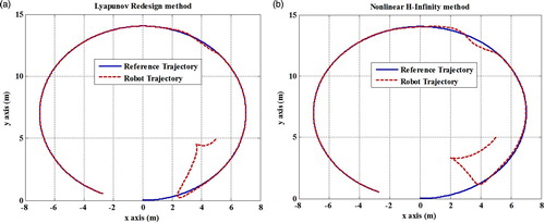
In this figure, it is evident that both methods are perfectly able to remain the robot on its reference trajectory; however, the proposed method (Lyapunov redesign method) is more robust to the side slip compared with nonlinear $H_{\mathrm{\infty }}$ control. Indeed, when the side slip has been happened as a disturbance, the max deviation from the reference trajectory in the proposed method is less than the other method. Moreover, Figure 4 shows the tracking errors ($e_1$ to $e_3$) for both methods. Since the tracking error has been defined as $e=T\left(q_r\left(t\right)-q\left(t\right)\right)$ and the matrix $T$ is non-singular, the convergence of $e_1$ to $e_3$ to zero, leads to converge of $q\left(t\right)$ to $q_r\left(t\right)$.

Figure 4. The resulting tracking errors (a) $e_1$, (b) $e_2$, (c) $e_3$, relating to Lyapunov redesign and nonlinear $H_{\mathrm{\infty }}$ methods.

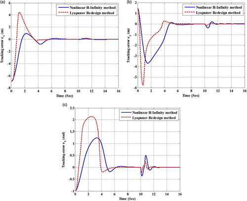
As seen in Figure 4, although the proposed method experiences higher transient peaks with respect to the nonlinear $H_{\mathrm{\infty }}$ control, in the initial seconds, it is more robust against the side slip. This robustness is the main goal of the paper.

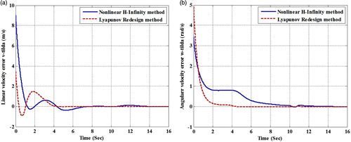
On the other hand, in the virtual control step it is desirable that $\tilde{v}$ and $\tilde{\omega }$ converge to zero, i.e. the linear and angular velocities of the robot will converge to their desired values ($v_d,{\omega }_d$). Figure 5 shows the errors of linear and angular velocities.

Figure 5. The resulting (a) linear velocity error ($\tilde{v}=v-v_d$) and (b) angular velocity error ($\tilde{\omega }=\omega -{\omega }_d$) relating to Lyapunov redesign and nonlinear $H_{\mathrm{\infty }}$ methods.

Control signals of the proposed methods are shown in Figure 6. Since $u_1={\tau }_1+{\tau }_2$ and $u_2={\tau }_1-{\tau }_2$, in simulation results in the torques ${\tau }_1$ and ${\tau }_2$ are shown.

Figure 6. The Control signals (a) ${\tau }_1$, (b) ${\tau }_2$ relating to Lyapunov redesign and nonlinear $H_{\mathrm{\infty }}$ methods.

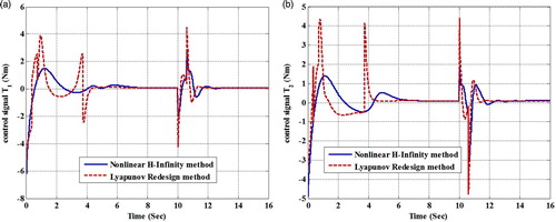
The goal of the proposed method is robustness against the side slip as an external disturbance. In Figure 6, it is seen that the control signals using the nonlinear $H_{\mathrm{\infty }}$ control are smoother with respect to Lyapunov redesign method. However, according to Figure 3, the proposed method is more robust to the side slip compared with nonlinear $H_{\mathrm{\infty }}$control. This is at the expense of having higher peaks in the control signal.

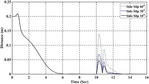
In Figure 7, the performance of Lyapunov redesign controller has been compared for different values of the side slip. In this figure, the distance of the robot from the reference path has been simulated for the side slips 10, 30 and 60 degrees which have been applied to the robot at the time t = 10 s.

Figure 7. The distance of the robot with the reference path using Lyapunov redesign methods for different values of side slip.

Remark 6.1:

In this paper, asymptotic stability has been considered for convergence of tracking error. Suggestions to improve this work are extending the results in the case of finite-time convergence of the error (Binazadeh and Shafiei, 2014b) and a mobile robot with slowly varying dynamic (Binazadeh and Shafiei, 2013). These trends have practical motivations in this field.

7. Conclusion

In this paper, a more realistic model compared with other references was considered for a nonholonomic mobile robot in the presence of side slip. Also, the Kanayama transformation was modified to have matched disturbances in equations of the tracking error. Then, a robust tracking controller using Lyapunov redesign method was designed for this robot. Moreover, in order to compare the proposed controller with an efficient nonlinear method, the nonlinear $H_{\mathrm{\infty }}$ control was developed for the robot with the side slip. It is worth noting that two proposed robust controllers were designed without any estimator or sensor to measure the slip value. The simulation results showed the effectiveness of the proposed controllers against the side slip and the asymptotic stability of tracking errors.

Disclosure statement

No potential conflict of interest was reported by the authors.

References

- Binazadeh, T., & Shafiei, M. H. (2013). Extending satisficing control strategy to slowly varying nonlinear systems. Communications in Nonlinear Science and Numerical Simulation, 18(4), 1071–1078. doi: 10.1016/j.cnsns.2012.07.025
- Binazadeh, T., & Shafiei, M. H. (2014a). Nonsingular terminal sliding-mode control of a tractor–trailer system. Systems Science & Control Engineering: An Open Access Journal, 2(1), 168–174. doi: 10.1080/21642583.2014.890552
- Binazadeh, T., & Shafiei, M. H. (2014b). A novel approach in the finite-time controller design. Systems Science & Control Engineering: An Open Access Journal, 2(1), 119–124. doi: 10.1080/21642583.2014.883946
- Chwa, D. (2004). Sliding-mode tracking control of nonholonomic wheeled mobile robots in polar coordinates. IEEE Transactions on Control Systems Technology, 12(4), 637–644. doi: 10.1109/TCST.2004.824953
- Do, K. D. (2013). Bounded controllers for global path tracking control of unicycle-type mobile robots. Robotics and Autonomous Systems, 61(8), 775–784. doi: 10.1016/j.robot.2013.04.014
- Du, H., Lam, J., Cheung, K.-C., Li, W., & Zhang, N. (2015). Side-slip angle estimation and stability control for a vehicle with a non-linear tyre model and a varying speed. Proceedings of the Institution of Mechanical Engineers, Part D: Journal of Automobile Engineering, 229(4), 486–505.
- Fierro, R., & Lewis, F. L. (1995). Control of a nonholonomic mobile robot: Backstepping kinematics into dynamics. IEEE Conference on Decision and Control, 4, 3805–3810.
- Hwang, E.-J., Kang, H.-S., Hyun, C.-H., & Park, M. (2013). Robust backstepping control based on a Lyapunov Redesign for Skid-Steered Wheeled Mobile Robots. International Journal of Advanced Robotic Systems, 10(1), 26. doi: 10.5772/55059
- JIANGdagger, Z.-P., & Nijmeijer, H. (1997). Tracking control of mobile robots: A case study in backstepping. Automatica, 33(7), 1393–1399. doi: 10.1016/S0005-1098(97)00055-1
- Kanayama, Y., Kimura, Y., Miyazaki, F., & Noguchi, T. (1990). A stable tracking control method for an autonomous mobile robot. In IEEE International Conference on Robotics and Automation (pp. 384–389). Cincinnati, OH: IEEE.
- Khalil, H. (2002). Nonlinear Systems (3rd edition). Upper Saddle River: Prentice hall.
- Li, S., Ding, L., Gao, H., Chen, C., Liu, Z., & Deng, Z. (2018). Adaptive neural network tracking control-based reinforcement learning for wheeled mobile robots with skidding and slipping. Neurocomputing, 283, 20–30. doi: 10.1016/j.neucom.2017.12.051
- Li, Y., Wang, Z., & Zhu, L. (2010). Adaptive neural network PID sliding mode dynamiccontrol of nonholonomic mobile robot. In Information and Automation (ICIA), 2010 IEEE International Conference on (pp. 753–757). Harbin, China: IEEE.
- Miyasato, Y. (2008). Adaptive H∞ control of nonholonomic mobile robot based on inverse optimality. In American Control Conference (pp. 3524–3529). Seattle, Washington: IEEE.
- Pourboghrat, F., & Karlsson, M. P. (2002). Adaptive control of dynamic mobile robots with nonholonomic constraints. Computers & Electrical Engineering, 28(4), 241–253. doi: 10.1016/S0045-7906(00)00053-7
- Slotine, J. J., & Li, W. (1991). Applied nonlinear control. vol. 199, no. 1. Englewood Cliffs, NJ: Prentice-Hall.
- Taheri-Kalani, J., & Khosrowjerdi, M. J. (2014). Adaptive trajectory tracking control of wheeled mobile robots with disturbance observer. International Journal of Adaptive Control and Signal Processing, 28(1), 14–27. doi: 10.1002/acs.2382
- Wang, D., & Low, C. B. (2008). Modeling and analysis of skidding and slipping in wheeled mobile robots: Control design perspective. IEEE Transactions on Robotics, 24(3), 676–687. doi: 10.1109/TRO.2008.921563
- Wang, T.-Y., & Tsai, C.-C. (2005). Adaptive robust control of Nonholonomic Wheeled Mobile Robots. 16th IFAC World Congress.
- Yang, J.-M., & Kim, J.-H. (1999). Sliding mode control for trajectory tracking of nonholonomic wheeled mobile robots. IEEE Transactions on Robotics and Automation, 15(3), 578–587. doi: 10.1109/70.768190
- Yoo, S. J. (2013). Adaptive neural tracking and obstacle avoidance of uncertain mobile robots with unknown skidding and slipping. Information Sciences, 238, 176–189. doi: 10.1016/j.ins.2013.03.013
- Zhou, B., Peng, Y., & Han, J. (2007). December. UKF based estimation and tracking control ofnonholonomic mobile robots with slipping. In IEEE International Conference on Robotics and Biomimetics (pp. 2058–2063). Sanya, China: IEEE.