The paradigm of complex probability and Monte Carlo methods

Abstract

In 1933, Andrey Nikolaevich Kolmogorov established the system of five axioms that define the concept of mathematical probability. This system can be developed to include the set of imaginary numbers and this by adding a supplementary three original axioms. Therefore, any experiment can be performed in the set $\mathcal{C}$ of complex probabilities which is the summation of the set $\mathcal{R}$ of real probabilities and the set $\mathcal{M}$ of imaginary probabilities. The purpose here is to include additional imaginary dimensions to the experiment taking place in the ‘real’ laboratory in $\mathcal{R}$ and hence to evaluate all the probabilities. Consequently, the probability in the entire set $\mathcal{C}$ = $\mathcal{R}$ + $\mathcal{M}$ is permanently equal to one no matter what the stochastic distribution of the input random variable in $\mathcal{R}$ is, therefore the outcome of the probabilistic experiment in $\mathcal{C}$ can be determined perfectly. This is due to the fact that the probability in $\mathcal{C}$ is calculated after subtracting from the degree of our knowledge the chaotic factor of the random experiment. This novel complex probability paradigm will be applied to the classical probabilistic Monte Carlo numerical methods and to prove as well the convergence of these stochastic procedures in an original way.

KEYWORDS:

• Complex set
• degree of our knowledge
• chaotic factor
• complex random vector
• probability norm
• simulation
• convergence probability
• divergence probability

Nomenclature

$\mathcal{R}$	=	real set of events
$\mathcal{M}$	=	imaginary set of events
$\mathcal{C}$	=	complex set of events
i	=	the imaginary number where $i=\sqrt{-1}$ or $i^2=-1$
EKA	=	Extended Kolmogorov's Axioms
CPP	=	Complex Probability Paradigm
Prob	=	probability of any event
Pr	=	probability in the real set $\mathcal{R}$ = probability of convergence in $\mathcal{R}$
Pm	=	probability in the imaginary set $\mathcal{M}$ corresponding to the real probability in $\mathcal{R}$ = probability of divergence in $\mathcal{M}$
Pc	=	probability of an event in $\mathcal{R}$ with its associated event in $\mathcal{M}$ = probability in the complex probability set $\mathcal{C}$
$R_E$	=	the exact result of the random experiment
$R_A$	=	the approximate result of the random experiment
z	=	complex probability number = sum of Pr and Pm = complex random vector
$DOK=|z{|}^2$	=	the degree of our knowledge of the random system or experiment, it is the square of the norm of z
Chf	=	the chaotic factor of z
MChf	=	magnitude of the chaotic factor of z
N	=	number of random vectors = number of iterations cycles
$N_C$	=	number of random vectors = number of iterations cycles till the convergence of Monte Carlo method to $R_E$
Z	=	the resultant complex random vector = $\sum _{j=1}^N{z}_j$
$DO{K}_Z=\frac{{|Z|}^2}{N^2}$	=	the degree of our knowledge of the whole stochastic system
$Ch{f}_Z=\frac{Chf}{N^2}$	=	the chaotic factor of the whole stochastic system
$MCh{f}_Z$	=	magnitude of the chaotic factor of the whole stochastic system
$Z_U$	=	the resultant complex random vector corresponding to a uniform random distribution
$DO{K}_{Z_U}$	=	the degree of our knowledge of the whole stochastic system corresponding to a uniform random distribution
$Ch{f}_{Z_U}$	=	the chaotic factor of the whole stochastic system corresponding to a uniform random distribution
$MCh{f}_{Z_U}$	=	the magnitude of the chaotic factor of the whole stochastic system corresponding to a uniform random distribution
$P{c}_U$	=	probability in the complex probability set $\mathcal{C}$ of the whole stochastic system corresponding to a uniform random distribution

I. Introduction

Firstly, in this introductory section an overview of Monte Carlo methods will be done. Before the Monte Carlo method was developed, simulations tested a previously understood deterministic problem, and statistical sampling was used to estimate uncertainties in the simulations. Monte Carlo simulations invert this approach, solving deterministic problems using a probabilistic analog (one can refer to Simulated annealing).

An early variant of the Monte Carlo method can be seen in the Buffon's needle experiment, in which π can be estimated by dropping needles on a floor made of parallel and equidistant strips. In the 1930s, Enrico Fermi first experimented with the Monte Carlo method while studying neutron diffusion, but did not publish anything on it (Metropolis, 1987).

The modern version of the Markov Chain Monte Carlo method was invented in the late 1940s by Stanislaw Ulam, while he was working on nuclear weapons projects at the Los Alamos National Laboratory. Immediately after Ulam's breakthrough, John von Neumann understood its importance and programmed the ENIAC computer to carry out Monte Carlo calculations. In 1946, physicists at Los Alamos Scientific Laboratory were investigating radiation shielding and the distance that neutrons would likely travel through various materials. Despite having most of the necessary data, such as the average distance a neutron would travel in a substance before it collided with an atomic nucleus, and how much energy the neutron was likely to give off following a collision, the Los Alamos physicists were unable to solve the problem using conventional, deterministic mathematical methods. Ulam had the idea of using random experiments. He recounts his inspiration as follows:

The first thoughts and attempts I made to practice [the Monte Carlo Method] were suggested by a question which occurred to me in 1946 as I was convalescing from an illness and playing solitaires. The question was what are the chances that a Canfield solitaire laid out with 52 cards will come out successfully? After spending a lot of time trying to estimate them by pure combinatorial calculations, I wondered whether a more practical method than ‘abstract thinking’ might not be to lay it out say one hundred times and simply observe and count the number of successful plays. This was already possible to envisage with the beginning of the new era of fast computers, and I immediately thought of problems of neutron diffusion and other questions of mathematical physics, and more generally how to change processes described by certain differential equations into an equivalent form interpretable as a succession of random operations. Later [in 1946], I described the idea to John von Neumann, and we began to plan actual calculations. (Eckhardt, 1987)

Being secret, the work of von Neumann and Ulam required a code name (Mazhdrakov, Benov, & Valkanov, 2018). A colleague of von Neumann and Ulam, Nicholas Metropolis, suggested using the name Monte Carlo, which refers to the Monte Carlo Casino in Monaco where Ulam's uncle would borrow money from relatives to gamble (Metropolis, 1987). Using lists of ‘truly random’ random numbers was extremely slow, but von Neumann developed a way to calculate pseudorandom numbers, using the middle-square method. Though this method has been criticized as crude, von Neumann was aware of this: he justified it as being faster than any other method at his disposal, and also noted that when it went awry it did so obviously, unlike methods that could be subtly incorrect (Peragine, 2013).

Monte Carlo methods were central to the simulations required for the Manhattan Project, though severely limited by the computational tools at the time. In the 1950s they were used at Los Alamos for early work relating to the development of the hydrogen bomb, and became popularized in the fields of physics, physical chemistry, and operations research. The Rand Corporation and the U.S. Air Force were two of the major organizations responsible for funding and disseminating information on Monte Carlo methods during this time, and they began to find a wide application in many different fields.

The theory of more sophisticated mean field type particle Monte Carlo methods had certainly started by the mid-1960s, with the work of Henry P. McKean Jr. on Markov interpretations of a class of nonlinear parabolic partial differential equations arising in fluid mechanics (McKean, 1967, 1966). We also quote an earlier pioneering article by Theodore E. Harris and Herman Kahn, published in 1951, using mean field genetic-type Monte Carlo methods for estimating particle transmission energies (Herman & Theodore, 1951). Mean field genetic type Monte Carlo methodologies are also used as heuristic natural search algorithms (also known as Metaheuristic) in evolutionary computing. The origins of these mean field computational techniques can be traced to 1950 and 1954 with the work of Alan Turing on genetic type mutation-selection learning machines (Turing, 1950) and the articles by Nils Aall Barricelli at the Institute for Advanced Study in Princeton, New Jersey (Barricelli, 1954, 1957).

Quantum Monte Carlo, and more specifically Diffusion Monte Carlo methods can also be interpreted as a mean field particle Monte Carlo approximation of Feynman-Kac path integrals (Assaraf, Caffarel, & Khelif, 2000; Caffarel, Ceperley, & Kalos, 1993; Del Moral, 2003; Del Moral, 2004; Del Moral & Miclo, 2000a, 2000b; Hetherington, 1984). The origins of Quantum Monte Carlo methods are often attributed to Enrico Fermi and Robert Richtmyer who developed in 1948 a mean field particle interpretation of neutron-chain reactions (Fermi & Richtmyer, 1948), but the first heuristic-like and genetic type particle algorithm (also known as Resampled or Reconfiguration Monte Carlo methods) for estimating ground state energies of quantum systems (in reduced matrix models) is due to Jack H. Hetherington in 1984 (Hetherington, 1984) In molecular chemistry, the use of genetic heuristic-like particle methodologies (also known as pruning and enrichment strategies) can be traced back to 1955 with the seminal work of Rosenbluth and Rosenbluth (1955).

The use of Sequential Monte Carlo in advanced signal processing and Bayesian inference is more recent. It was in 1993, that Gordon et al., published in their seminal work (Gordon, Salmond, & Smith, 1993) the first application of a Monte Carlo resampling algorithm in Bayesian statistical inference. The authors named their algorithm ‘the bootstrap filter’, and demonstrated that compared to other filtering methods, their bootstrap algorithm does not require any assumption about that state-space or the noise of the system. We also quote another pioneering article in this field of Genshiro Kitagawa on a related ‘Monte Carlo filter’ (Kitagawa, 1996), and the ones by Pierre Del Moral (1996) and Carvalho, Del Moral, Monin, and Salut (1997) on particle filters published in the mid-1990s. Particle filters were also developed in signal processing in the early 1989–1992 by P. Del Moral, J.C. Noyer, G. Rigal, and G. Salut in the LAAS-CNRS in a series of restricted and classified research reports with STCAN (Service Technique des Constructions et Armes Navales), the IT company DIGILOG, and the LAAS-CNRS (the Laboratory for Analysis and Architecture of Systems) on RADAR/SONAR and GPS signal processing problems (Del Moral, Noyer, Rigal, & Salut, 1992c; Del Moral, Rigal, & Salut, 1991, September; Del Moral, Rigal, & Salut, 1991, April; Del Moral, Rigal, & Salut, 1992, October; Del Moral, Rigal, & Salut, 1992, January; Del Moral, Rigal, & Salut, 1993). These Sequential Monte Carlo methodologies can be interpreted as an acceptance–rejection sampler equipped with an interacting recycling mechanism.

From 1950 to 1996, all the publications on Sequential Monte Carlo methodologies including the pruning and resample Monte Carlo methods introduced in computational physics and molecular chemistry, present natural and heuristic-like algorithms applied to different situations without a single proof of their consistency, nor a discussion on the bias of the estimates and on genealogical and ancestral tree-based algorithms. The mathematical foundations and the first rigorous analysis of these particle algorithms are due to Del Moral (1996, 1998) in 1996. Branching type particle methodologies with varying population sizes were also developed in the end of the 1990s by Dan Crisan, Jessica Gaines and Terry Lyons (Crisan & Lyons, 1997, 1999; Crisan, Gaines, & Lyons, 1998) and by Crisan, Del Moral, and Lyons (1999), Further developments in this field were developed in 2000 by P. Del Moral, A. Guionnet and L. Miclo (Del Moral & Guionnet, 1999, 2001; Del Moral & Miclo, 2000a).

Finally, and to conclude, this research work is organized as follows: After the introduction in section 1, the purpose and the advantages of the present work are presented in section 2. Afterward, in section 3, we will explain and illustrate the complex probability paradigm with its original parameters and interpretation. In section 4, the Monte Carlo techniques of integration and simulation will be explained. In section 5, I will extend Monte Carlo methods to the imaginary and complex probability sets and hence link this concept to my novel complex probability paradigm. Moreover, in section 6, I will prove the convergence of Monte Carlo methods using the concept of the resultant complex random vector Z. Furthermore, in section 7 we will evaluate the original paradigm parameters and in section 8 a flowchart of the complex probability and Monte Carlo methods prognostic model will be drawn. Additionally, in section 9 simulations of Monte Carlo methods will be accomplished in the continuous and discrete cases. Finally, I conclude the work by doing a comprehensive summary in section 10, and then present the list of references cited in the current research work.

II. The purpose and the advantages of the present work

In this section we will present the purpose and the advantages of the current research work. Computing probabilities is the main work of classical probability theory. Adding new dimensions to the stochastic experiments will lead to a deterministic expression of probability theory. This is the original idea at the foundations of this work. Actually, the theory of probability is a nondeterministic system in its essence; that means that the events outcomes are due to chance and randomness. The addition of novel imaginary dimensions to the chaotic experiment occurring in the set $\mathcal{R}$ will yield a deterministic experiment and hence a stochastic event will have a certain result in the complex probability set $\mathcal{C}$. If the random event becomes completely predictable then we will be fully knowledgeable to predict the outcome of stochastic experiments that arise in the real world in all stochastic processes. Consequently, the work that has been accomplished here was to extend the real probabilities set $\mathcal{R}$ to the deterministic complex probabilities set $\mathcal{C}$ = $\mathcal{R}$ + $\mathcal{M}$ by including the contributions of the set $\mathcal{M}$ which is the imaginary set of probabilities. Therefore, since this extension was found to be successful, then a novel paradigm of stochastic sciences and prognostic was laid down in which all stochastic phenomena in $\mathcal{R}$ was expressed deterministically. I called this original model ‘the Complex Probability Paradigm’ that was initiated and illustrated in my twelve research publications (Abou Jaoude, 2013a, 2013b, 2014, 2015a, 2015b, 2016a, 2016b, 2017a, 2017b, 2017c, 2018; Abou Jaoude, El-Tawil, & Kadry, 2010).

Accordingly, the advantages and the purpose of the current paper are to:

1. Extend classical probability theory to the set of complex numbers, therefore to link the theory of probability to the field of complex variables and analysis. This job was started and elaborated in my previous twelve papers.

2. Apply the new axioms of probability and paradigm to Monte Carlo methods.

3. Show that all stochastic phenomena can be expressed deterministically in the set of complex probabilities $\mathcal{C}$.

4. Measure and compute both the degree of our knowledge and the chaotic factor of Monte Carlo methods.

5. Draw and illustrate the graphs of the parameters and functions of the original paradigm corresponding to Monte Carlo methods.

6. Show that the classical concept of probability is always equal to one in the complex set; hence, no randomness, no chaos, no uncertainty, no ignorance, no disorder, and no unpredictability exist in: $\mathcal{C}\left(\text{complex}\text{set}\right)=\mathcal{R}\left(\text{real}\text{set}\right)+\mathcal{M}\left(\text{imaginary}\text{set}\right)$

7. Prove the convergence of the stochastic Monte Carlo procedures in an original way by using the newly defined axioms and paradigm.

8. Pave the way to implement this novel model to other areas in stochastic processes and to the field of prognostics. These will be the topics of my future research works.

Concerning some applications of the original elaborated paradigm and as a future work, it can be applied to any random phenomena using Monte Carlo methods whether in the discrete or in the continuous cases.

Furthermore, compared with existing literature, the main contribution of the present research work is to apply the novel paradigm of complex probability to the concepts and techniques of the stochastic Monte Carlo methods and simulations.

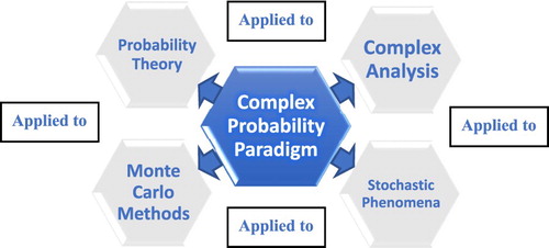
The following figure shows the main purposes of the Complex Probability Paradigm (CPP) (Figure 1).

Figure 1. The diagram of the main purposes of the Complex Probability Paradigm.

III. The complex probability paradigm

III.1. The original Andrey Nikolaevich Kolmogorov system of axioms

The simplicity of Kolmogorov’s system of axioms may be surprising. Let E be a collection of elements {E₁, E₂, … } called elementary events and let F be a set of subsets of E called random events. The five axioms for a finite set E are (Benton, 1966a, 1966b; Feller, 1968; Freund, 1973; Montgomery & Runger, 2003; Walpole, Myers, Myers, & Ye, 2002):

Axiom 1: F is a field of sets.

Axiom 2: F contains the set E.

Axiom 3: A non-negative real number P_rob(A), called the probability of A, is assigned to each set A in F. We have always 0 ≤ P_rob(A) ≤ 1.

Axiom 4: P_rob(E) equals 1.

Axiom 5: If A and B have no elements in common, the number assigned to their union is: $P_{\text{rob}}(A\cup B)=P_{\text{rob}}\left(A\right)+P_{\text{rob}}\left(B\right)$ hence, we say that A and B are disjoint; otherwise, we have: $P_{\text{rob}}(A\cup B)=P_{\text{rob}}\left(A\right)+P_{\text{rob}}\left(B\right)-P_{\text{rob}}(A\cap B)$ And we say also that: $P_{\text{rob}}(A\cap B)=P_{\text{rob}}\left(A\right)\times P_{\text{rob}}\left(B/A\right)=P_{\text{rob}}\left(B\right)\times P_{\text{rob}}\left(A/B\right)$ which is the conditional probability. If both A and B are independent then: $P_{\text{rob}}(A\cap B)=P_{\text{rob}}\left(A\right)\times P_{\text{rob}}\left(B\right)$.

Moreover, we can generalize and say that for N disjoint (mutually exclusive) events $A_1,A_2,\dots ,A_j,\dots ,A_N$ (for $1\le j\le N$), we have the following additivity rule: $P_{\text{rob}}\left(\bigcup _{j=1}^N{A}_j\right)=\sum _{j=1}^N{P}_{\text{rob}}\left(A_j\right)$ And we say also that for N independent events $A_1,A_2,\dots ,A_j,\dots ,A_N$ (for $1\le j\le N$), we have the following product rule: $P_{\text{rob}}\left(\bigcap _{j=1}^N{A}_j\right)=\prod _{j=1}^N{P}_{\text{rob}}\left(A_j\right)$

III.2. Adding the imaginary part $\mathcal{M}$

Now, we can add to this system of axioms an imaginary part such that:

Axiom 6: Let $P_m=i\times (1-P_r)$ be the probability of an associated event in $\mathcal{M}$ (the imaginary part) to the event A in $\mathcal{R}$ (the real part). It follows that $P_r+P_m/i=1$ where i is the imaginary number with $i=\sqrt{-1}$ or $i^2=-1$.

Axiom 7: We construct the complex number or vector $Z=P_r+P_m=P_r+i(1-P_r)$ having a norm $|Z|$ such that: $|Z{|}^2=P_r^2+(P_m/i{)}^2.$

Axiom 8: Let Pc denote the probability of an event in the complex probability universe $\mathcal{C}$ where $\mathcal{C}$ = $\mathcal{R}$ + $\mathcal{M}$. We say that Pc is the probability of an event A in $\mathcal{R}$ with its associated event in $\mathcal{M}$ such that: $\begin{array}{rl}P{c}^2& ={\left(P_r+\frac{P_m}{i}\right)}^2\\ & =|Z{|}^2-2i{P}_r{P}_m\text{and}\text{is}\text{always}\text{equal}\text{to}1.\end{array}$ We can see that by taking into consideration the set of imaginary probabilities we added three new and original axioms and consequently the system of axioms defined by Kolmogorov was hence expanded to encompass the set of imaginary numbers.

III.3. The purpose of extending the axioms

After adding the new three axioms, it becomes clear that the addition of the imaginary dimensions to the real stochastic experiment yields a probability always equal to one in the complex probability set $\mathcal{C}$. Actually, we will understand directly this result when we realize that the set of probabilities is formed now of two parts: the first part is real and the second part is imaginary. The stochastic event that is happening in the set $\mathcal{R}$ of real probabilities (like in the experiment of coin tossing and getting a tail or a head) has a corresponding real probability $P_r$ and a corresponding imaginary probability $P_m$. In addition, let $\mathcal{M}$ be the set of imaginary probabilities and let $|Z{|}^2$ be the Degree of Our Knowledge (DOK for short) of this experiment. According to the axioms of Kolmogorov, $P_r$ is always the probability of the phenomenon in the set $\mathcal{R}$ (Barrow, 1992; Bogdanov & Bogdanov, 2009; Srinivasan & Mehata, 1988; Stewart, 1996; Stewart, 2002; Stewart, 2012).

• In fact, a total ignorance of the set $\mathcal{M}$ leads to:

  P_rob(event) $=P_r=0.5$, $P_m$ = P_rob(imaginary part) = 0.5i, and $|Z{|}^2=DOK$ in this case is equal to: $1-2P_r(1-P_r)=1-(2\times 0.5)\times (1-0.5)=0.5$

• Conversely, a total knowledge of the set in $\mathcal{R}$ leads to:

  P_rob(event) $=P_r=1$ and $P_m$ = P_rob(imaginary part) = 0. Here we have $DOK=1-(2\times 1)\times (1-1)=1$ because the phenomenon is totally known, that is, all the variables and laws affecting the experiment are determined completely, therefore; our degree of our knowledge (DOK) of the system is 1 = 100%.

• Now, if we are sure that an event will never happen i.e. like ‘getting nothing’ (the empty set), $P_r$ is accordingly = 0, that is, the event will never occur in $\mathcal{R}$. $P_m$ will be equal to: $i(1-P_r)=i(1-0)=i$, and $|Z{|}^2=DOK=1-(2\times 0)\times (1-0)=1$, because we are sure that the event of getting nothing will never happen; therefore, the Degree of Our Knowledge (DOK) of the system is 1 = 100%.

We can deduce that we have always: $0.5\le |Z{|}^2\le 1,\mathrm{\forall }{P}_r:0\le P_r\le 1$ and $|Z{|}^2=DOK=P_r^2+(P_m/i{)}^2$, where $0\le P_r,P_m/i\le 1$.

And what is crucial is that in all cases we have: $\begin{array}{rl}P{c}^2& ={\left(P_r+\frac{P_m}{i}\right)}^2=|Z{|}^2-2i{P}_r{P}_m\\ & =[P_r+(1-P_r){]}^2=1^2=1\end{array}$ Actually, according to an experimenter in $\mathcal{R}$, the phenomenon is random: the experimenter ignores the outcome of the chaotic phenomenon. Each outcome will be assigned a probability $P_r$ and he will say that the outcome is nondeterministic. But in the complex probability universe $\mathcal{C}$ = $\mathcal{R}$ + $\mathcal{M}$, the outcome of the random phenomenon will be totally predicted by the observer since the contributions of the set $\mathcal{M}$ were taken into consideration, so this will give: $P{c}^2={\left(P_r+\frac{P_m}{i}\right)}^2$

Therefore $Pc$ is always equal to 1. Actually, adding the imaginary set to our stochastic phenomenon leads to the elimination of randomness, of ignorance, and of nondeterminism. Subsequently, conducting experiments of this class of phenomena in the set $\mathcal{C}$ is of great importance since we will be able to foretell with certainty the output of all random phenomenon. In fact, conducting experiments in the set $\mathcal{R}$ leads to uncertainty and unpredictability. So, we place ourselves in the set $\mathcal{C}$ instead of placing ourselves in the set $\mathcal{R}$, then study the random events, since in $\mathcal{C}$ we take into consideration all the contributions of the set $\mathcal{M}$ and therefore a deterministic study of the stochastic experiment becomes possible. Conversely, by taking into consideration the contributions of the probability set $\mathcal{M}$ we place ourselves in the set $\mathcal{C}$ and by disregarding $\mathcal{M}$ we restrict our experiment to nondeterministic events in $\mathcal{R}$ (Bell, 1992; Bogdanov & Bogdanov, 2010; Bogdanov & Bogdanov, 2012; Bogdanov & Bogdanov, 2013; Boursin, 1986; Dacunha-Castelle, 1996; Dalmedico-Dahan, Chabert, & Chemla, 1992; Ekeland, 1991; Gleick, 1997; Van Kampen, 2006).

Furthermore, we can deduce from the above axioms and definitions that: $\begin{array}{rl}2i{P}_r{P}_m& =2i\times P_r\times i\times (1-P_r)\\ & =2i^2\times P_r\times (1-P_r)=-2P_r(1-P_r)\\ & =Chf\end{array}$ $2i{P}_r{P}_m$ will be called the Chaotic factor in our stochastic event and will be denoted accordingly by ‘Chf’. We will understand why we have named this term the chaotic factor; in fact:

• In case P_r = 1, that means in the case of a certain event, then the chaotic factor of the event is equal to 0.

• In case P_r = 0, that means in the case of an impossible event, then Chf = 0. Therefore, in both two last cases, there is no chaos because the output of the event is certain and is known in advance.

• In case P_r = 0.5, Chf = −0.5.

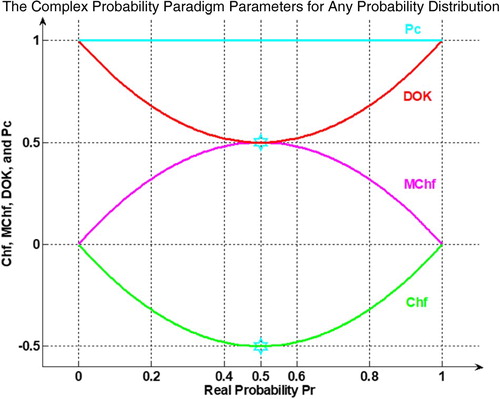
So, we deduce that: $-0.5\le Chf\le 0,\mathrm{\forall }{P}_r:0\le P_r\le 1$. (Figures 2–4)

Figure 2. Chf, DOK, and Pc for any probability distribution in 2D.

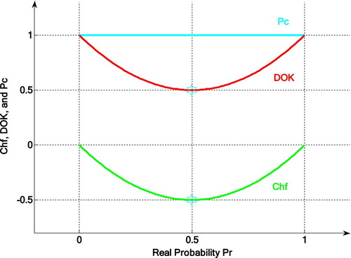
Figure 3. DOK, Chf, and Pc for any probability distribution in 3D with $P{c}^2=DOK-Chf=1=Pc$.

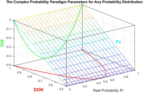
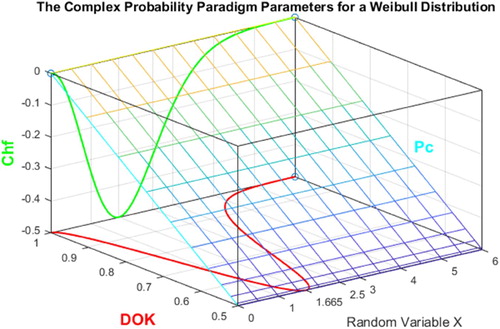
Figure 4. DOK, Chf, and Pc for a Weibull probability distribution in 3D with $P{c}^2=DOK-Chf=1=Pc$.

Consequently, what is truly interesting here is therefore we have quantified both the degree of our knowledge and the chaotic factor of any stochastic phenomenon and hence we can state accordingly: $P{c}^2=|Z{|}^2-2i{P}_r{P}_m=DOK-Chf$ Then we can conclude that: $\begin{array}{rl}P{c}^2& =\text{Degree}\text{of}\text{our}\text{knowledge}\text{of}\text{the}\text{system}\text{--}\\ & \text{Chaotic}\text{factor}=1,\end{array}$ therefore $Pc=1$ permanently and constantly.

This directly leads to the following crucial conclusion: if we succeed to subtract and eliminate the chaotic factor in any stochastic phenomenon, then we will have the outcome probability always equal to one (Abou Jaoude, 2013a, 2013b, 2014, 2015a, 2015b, 2016a, 2016b, 2017a, 2017b, 2017c, 2018; Abou Jaoude et al., 2010) (Dalmedico-Dahan & Peiffer, 1986; Davies, 1993; Gillies, 2000; Guillen, 1995; Gullberg, 1997; Hawking, 2002, 2005, 2011; Pickover, 2008; Science Et Vie, 1999).

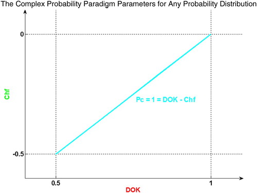
The graph below illustrates the linear relation between both DOK and Chf. (Figure 5)

Figure 5. Graph of $P{c}^2=DOK-Chf=1=Pc$ for any probability distribution.

Furthermore, we require in our present analysis the absolute value of the chaotic factor that will quantify for us the magnitude of the chaotic and stochastic influences on the random system considered which is materialized by the real probability $P_r$ and a probability density function, and which lead to an increasing or decreasing system chaos in $\mathcal{R}$. This additional and original term will be denoted accordingly MChf or Magnitude of the Chaotic factor. Therefore, we define this new term by: $\begin{array}{rl}MChf& =|Chf|=|2i{P}_r{P}_m|\\ & =-2i{P}_r{P}_m=2P_r(1-P_r)\ge 0,\mathrm{\forall }{P}_r:0\le P_r\le 1,\end{array}$ and $\begin{array}{rl}P{c}^{\text{2}}& =DOK-Chf\\ & =DOK+|Chf|,\text{since}-\text{0}\text{.5}\le Chf\le \text{0 }\\ & =DOK+MChf=\text{1,}\end{array}$ $\iff \text{0}\le MChf\le \text{0}\text{.5}$ where $\text{0}\text{.5}\le DOK\le \text{1}$.

The graph below (Figure 6) illustrates the linear relation between both DOK and MChf. Moreover, Figures 7–13 illustrate the graphs of Chf, MChf, DOK, and Pc as functions of the real probability P_r and of the random variable X for any probability distribution and for a Weibull probability distribution (Abou Jaoude, 2013a, 2013b, 2014, 2015a, 2015b, 2016a, 2016b, 2017a, 2017b, 2017c, 2018; Abou Jaoude et al., 2010).

Figure 6. Graph of $P{c}^2=DOK+MChf=1=Pc$ for any probability distribution.

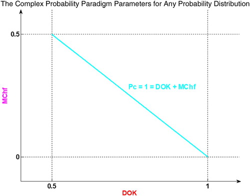
Figure 7. MChf, DOK, and Pc for any probability distribution in 2D.

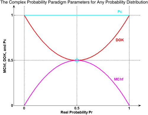
Figure 8. DOK, MChf, and Pc for any probability distribution in 3D with $P{c}^2=DOK+MChf=1=Pc$.

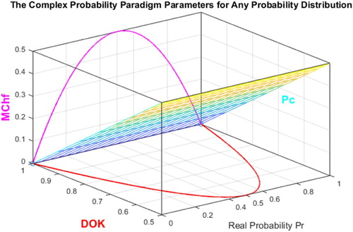
Figure 9. DOK, MChf, and Pc for a Weibull probability distribution in 3D with $P{c}^2=DOK+MChf=1=Pc$.

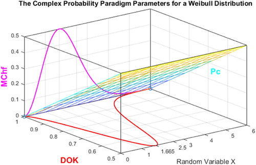
Figure 10. Chf and MChf for any probability distribution in 2D.

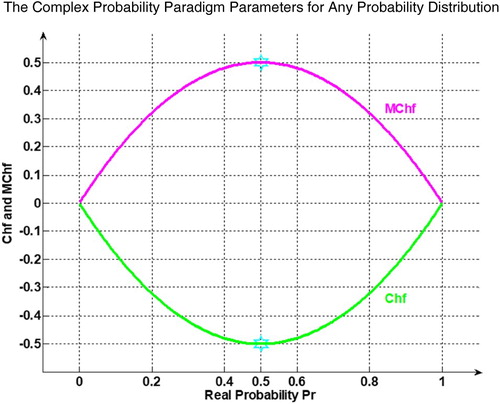
Figure 11. Chf and MChf for any probability distribution in 3D with MChf + Chf = 0.

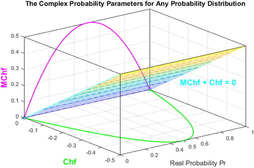
Figure 12. Chf and MChf for a Weibull probability distribution in 3D with MChf + Chf = 0.

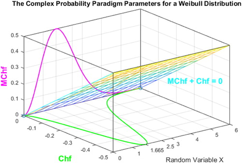
Figure 13. Chf, MChf, DOK, and Pc for any probability distribution in 2D.

To conclude and to summarize, in the real probability universe $\mathcal{R}$ our degree of our certain knowledge is regrettably imperfect, therefore we extend our study to the complex set $\mathcal{C}$ which embraces the contributions of both the real probabilities set $\mathcal{R}$ and the imaginary probabilities set $\mathcal{M}$. Subsequently, this will lead to a perfect and complete degree of knowledge in the universe $\mathcal{C}$ = $\mathcal{R}$ + $\mathcal{M}$ (since Pc = 1). In fact, working in the complex universe $\mathcal{C}$ leads to a certain prediction of any random event, because in $\mathcal{C}$ we eliminate and subtract from the calculated degree of our knowledge the quantified chaotic factor. 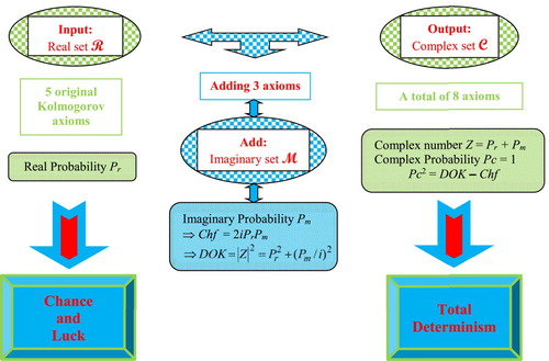This will yield a probability in the universe $\mathcal{C}$ equal to one (Pc²= DOK−Chf = DOK + MChf = 1 = Pc). Many illustrations considering various continuous and discrete probability distributions in my twelve previous research papers verify this hypothesis and novel paradigm (Abou Jaoude, 2013a, 2013b, 2014, 2015a, 2015b, 2016a, 2016b, 2017a, 2017b, 2017c, 2018; Abou Jaoude et al., 2010). The Extended Kolmogorov Axioms (EKA for short) or the Complex Probability Paradigm (CPP for short) can be summarized and shown in the following figure (Figure 14):

Figure 14. The EKA or the CPP diagram.

IV. The Monte Carlo techniques of integration and simulation (Gentle, 2003; Monte Carlo Method; Probability; Probability Axioms; Probability Density Function; Probability Distribution; Probability Interpretations; Probability Measure; Probability Theory; Stochastic Process; Probability Space Wikipedia)

In applied mathematics, the name Monte Carlo is given to the method of solving problems by means of experiments with random numbers. This name, after the casino at Monaco, was first applied around 1944 to the method of solving deterministic problems by reformulating them in terms of a problem with random elements which could then be solved by large-scale sampling. But, by extension, the term has come to mean any simulation that uses random numbers.

The development and proliferation of computers has led to the widespread use of Monte Carlo methods in virtually all branches of science, ranging from nuclear physics (where computer-aided Monte Carlo was first applied) to astrophysics, biology, engineering, medicine, operations research, and the social sciences.

The Monte Carlo Method of solving problems by using random numbers in a computer – either by direct simulation of physical or statistical problems or by reformulating deterministic problems in terms of one incorporating randomness – has become one of the most important tools of applied mathematics and computer science. A significant proportion of articles in technical journals in such fields as physics, chemistry, and statistics contain articles reporting results of Monte Carlo simulations or suggestions on how they might be applied. Some journals are devoted almost entirely to Monte Carlo problems in their fields. Studies in the formation of the universe or of stars and their planetary systems use Monte Carlo techniques. Studies in genetics, the biochemistry of DNA, and the random configuration and knotting of biological molecules are studied by Monte Carlo methods. In number theory, Monte Carlo methods play an important role in determining primality or factoring of very large integers far beyond the range of deterministic methods. Several important new statistical techniques such as ‘bootstrapping’ and ‘jackknifing’ are based on Monte Carlo methods.

Hence, the role of Monte Carlo methods and simulation in all of the sciences has increased in importance during the past several years. These methods play a central role in the rapidly developing subdisciplines of the computational physical sciences, the computational life sciences, and the other computational sciences. Therefore, the growing power of computers and the evolving simulation methodology have led to the recognition of computation as a third approach for advancing the natural sciences, together with theory and traditional experimentation. At the kernel of Monte Carlo simulation is random number generation.

Now we turn to the approximation of a definite integral by the Monte Carlo method. If we select the first N elements $x_1,x_2,\dots ,x_N$ from a random sequence in the interval (0,1), then: ${\int }_0^{1}f\left(x\right).\text{d}x\cong \frac{(1-0)}{N}\sum _{j=1}^{N}f\left(x_j\right)=\frac{1}{N}\sum _{j=1}^{N}f\left(x_j\right)$ Here the integral is approximated by the average of N numbers $f\left(x_1\right),f\left(x_2\right),\dots ,f\left(x_N\right)$. When this is actually carried out, the error is of order $1/\sqrt{N}$, which is not at all competitive with good algorithms, such as the Romberg method. However, in higher dimensions, the Monte Carlo method can be quite attractive. For example, $\begin{array}{rl}& {\int }_0^1{\int }_0^1{\int }_0^{1}f(x,y,z).\text{d}x.\text{d}y.\text{d}z\\ & \cong \frac{\left[\right(1-0)\times (1-0)\times (1-0\left)\right]}{N}\sum _{j=1}^{N}f(x_j,y_j,z_j)\\ & =\frac{1}{N}\sum _{j=1}^{N}f(x_j,y_j,z_j)\end{array}$ where $(x_j,y_j,z_j)$ is a random sequence of N points in the unit cube $0\le x\le 1$, $0\le y\le 1$, and $0\le z\le 1$. To obtain random points in the cube, we assume that we have a random sequence in (0,1) denoted by ${\xi }_1,{\xi }_2,{\xi }_3,{\xi }_4,{\xi }_5,{\xi }_6,\dots$To get our first random point $p_1$ in the cube, just let $p_1=({\xi }_1,{\xi }_2,{\xi }_3)$. The second is, of course, $p_2=({\xi }_4,{\xi }_5,{\xi }_6)$ and so on.

If the interval (in a one-dimensional integral) is not of length 1, but say is the general case (a, b), then the average of f over N random points in (a, b) is not simply an approximation for the integral but rather for: $\frac{1}{b-a}{\int }_a^{b}f\left(x\right).\text{d}x$ which agrees with our intention that the function $f\left(x\right)=1$ has an average of 1. Similarly, in higher dimensions, the average of f over a region is obtained by integrating and dividing by the area, volume, or measure of that region. For instance, $\begin{array}{rl}& \frac{1}{\left[\right(7-4)\times (5-(-2))\times (3-0\left)\right]}\\ & \times {\int }_4^7{\int }_{-2}^5{\int }_0^{3}f(x,y,z).\text{d}x.\text{d}y.\text{d}z\\ & =\frac{1}{63}{\int }_4^7{\int }_{-2}^5{\int }_0^{3}f(x,y,z).\text{d}x.\text{d}y.\text{d}z\end{array}$ is the average of f over the parallelepiped described by the following three inequalities: $0\le x\le 3,-2\le y\le 5,4\le z\le 7.$ To keep the limits of integration straight, we recall that: ${\int }_a^b{\int }_c^{d}f(x,y).\text{d}x.\text{d}y={\int }_a^b\left[{\int }_c^{d}f(x,y).\text{d}x\right].\text{d}y$ and $\begin{array}{rl}& {\int }_{a1}^{a2}{\int }_{b1}^{b2}{\int }_{c1}^{c2}f(x,y,z).\text{d}x.\text{d}y.\text{d}z\\ & ={\int }_{a1}^{a1}\left\{{\int }_{b1}^{b2}\left[{\int }_{c1}^{c2}f(x,y,z).\text{d}x\right].\text{d}y\right\}.\text{d}z\end{array}$ So, if $(x_j,y_j)$ denote random points with appropriate uniform distribution, the following examples illustrate Monte Carlo techniques: ${\int }_1^{9}f\left(x\right).\text{d}x\cong \frac{(9-1)}{N}\sum _{j=1}^{N}f\left(x_j\right)=\frac{8}{N}\sum _{j=1}^{N}f\left(x_j\right)$ $\begin{array}{rl}{\int }_4^8{\int }_2^{5}f(x,y).\text{d}x.\text{d}y& \cong \frac{\left[\right(8-4)\times (5-2\left)\right]}{N}\sum _{j=1}^{N}f(x_j,y_j)\\ & =\frac{12}{N}\sum _{j=1}^{N}f(x_j,y_j)\end{array}$ In each case, the random points should be uniformly distributed in the regions involved.

In general, we have: $\begin{array}{rl}& {\int }_{A}f\cong \left(\text{measure}\text{of}A\right)\\ & \times \left(\text{average}\text{of}f\text{over}N\text{random}\text{points}\text{in}A\right)\end{array}$ Here we are using the fact that the average of a function on a set is equal to the integral of the function over the set divided by the measure of the set.

V. The complex probability paradigm and Monte Carlo methods parameters (Abou Jaoude, 2013a, 2013b, 2014, 2015a, 2015b, 2016a, 2016b, 2017a, 2017b, 2017c, 2018, 2019a, 2019b; Abou Jaoude et al., 2010; Bidabad, 1992; Chan Man Fong, De Kee, & Kaloni, 1997; 2004, 2005, 2007; Cox, 1955; Fagin, Halpern, & Megiddo, 1990; Ognjanović, Marković, Rašković, Doder, & Perović, 2012; Stepić & Ognjanović, 2014; Wei, Park, Qiu, Wu, & Jung, 2017; Wei, Qiu, Karimi, & Ji, 2017; Weingarten, 2002; Youssef, 1994)

V.1. The probabilities of convergence and divergence

Let $R_E$ be the exact result of the random experiment or of a simple or a multidimensional integral that are not always possible to evaluate by ordinary methods of probability theory or calculus or deterministic numerical methods. And let $R_A$ be the approximate result of these experiments and integrals found by Monte Carlo methods.

The relative error in the Monte Carlo methods is: $\text{Rel}\text{. Error }=\left|\frac{R_E-R_A}{R_E}\right|=\left|1-\frac{R_A}{R_E}\right|$

In addition, the percent relative error is $=100\mathrm{\%}\times |\left(R_E-R_A\right)/R_E|$ and is always between 0% and 100%. Therefore, the relative error is always between 0 and 1. Hence: $\begin{array}{rl}0& \le \left|\frac{R_E-R_A}{R_E}\right|\le 1\\ & \iff \left\{\begin{array}{ll}0\le \left(\frac{R_E-R_A}{R_E}\right)\le 1& \text{if}{R}_A\le R_E\\ 0\le -\left(\frac{R_E-R_A}{R_E}\right)\le 1& \text{if}{R}_A\ge R_E\end{array}\right.\\ & \iff \left\{\begin{array}{l}0\le R_A\le R_E\\ R_E\le R_A\le 2R_E\end{array}\right.\end{array}$ Moreover, we define the real probability by: $\begin{array}{rl}{P}_r& =1-\left|\frac{R_E-R_A}{R_E}\right|=1-\left|1-\frac{R_A}{R_E}\right|\\ & =\left\{\begin{array}{ll}1-\left(1-\frac{R_A}{R_E}\right)& \text{if}\text{0}\le R_A\le R_E\\ 1+\left(1-\frac{R_A}{R_E}\right)& \text{if }{R}_E\le R_A\le 2R_E\end{array}\right.\\ & =\left\{\begin{array}{ll}\frac{R_A}{R_E}& \text{if}\text{0}\le R_A\le R_E\\ 2-\frac{R_A}{R_E}& \text{if}{R}_E\le R_A\le 2R_E\end{array}\right.\end{array}$

= 1 – the relative error in the Monte Carlo method

= Probability of Monte Carlo method convergence in $\mathcal{R}$.

And therefore: $\begin{array}{rl}{P}_m& =i\left(1-P_r\right)=i\left\{1-\left[1-\left|\frac{R_E-R_A}{R_E}\right|\right]\right\}\\ & =i\left\{1-\left[1-\left|1-\frac{R_A}{R_E}\right|\right]\right\}=i\left|1-\frac{R_A}{R_E}\right|\\ & =\left\{\begin{array}{ll}i\left(1-\frac{R_A}{R_E}\right)& \text{if}\text{0}\le R_A\le R_E\\ -i\left(1-\frac{R_A}{R_E}\right)& \text{if}{R}_E\le R_A\le 2R_E\end{array}\right.\\ & =\left\{\begin{array}{ll}i\left(1-\frac{R_A}{R_E}\right)& \text{if}\text{0}\le R_A\le R_E\\ i\left(\frac{R_A}{R_E}-1\right)& \text{if}{R}_E\le R_A\le 2R_E\end{array}\right.\end{array}$ = Probability of Monte Carlo method divergence in the imaginary probability set $\mathcal{M}$ since it is the imaginary complement of $P_r$.

Consequently, $\begin{array}{rl}\frac{P_m}{i}& =1-P_r=\left|1-\frac{R_A}{R_E}\right|\\ & =\left\{\begin{array}{ll}1-\frac{R_A}{R_E}& \text{if}\text{0}\le R_A\le R_E\\ \frac{R_A}{R_E}-1& \text{if}{R}_E\le R_A\le 2R_E\end{array}\right.\end{array}$ = The relative error in the Monte Carlo method

= Probability of Monte Carlo method divergence in $\mathcal{R}$ since it is the real complement of $P_r$.

In the case where $0\le R_A\le R_E$ we have $0\le \frac{R_A}{R_E}\le 1\Rightarrow 0\le P_r\le 1$ and we deduce also that $0\le \left(1-\frac{R_A}{R_E}\right)\le 1\Rightarrow 0\le P_m/i\le 1$ and $\Rightarrow 0\le P_m\le i$.

And in the case where $R_E\le R_A\le 2R_E\Rightarrow 1\le \frac{R_A}{R_E}\le 2\Rightarrow 0\le P_r\le 1$ and we deduce also that $0\le \left(\frac{R_A}{R_E}-1\right)\le 1\Rightarrow 0\le P_m/i\le 1$ and $\Rightarrow 0\le P_m\le i$

Therefore, if $R_A=0$ or $R_A=2R_E$ that means before the beginning of the simulation, then:

$P_r$ = P_rob (convergence) in $\mathcal{R}$ = 0

$P_m$ = P_rob (divergence) in $\mathcal{M}$ = i

$P_m/i$ = P_rob (divergence) in $\mathcal{R}$ = 1

And if $R_A=R_E$ that means at the end of Monte Carlo simulation then:

$P_r$ = P_rob (convergence) in $\mathcal{R}$ = 1

$P_m$ = P_rob (divergence) in $\mathcal{M}$ = 0

$P_m/i$ = P_rob (divergence) in $\mathcal{R}$ = 0

V.2. The complex random vector Z in $\mathcal{C}$

We have $\begin{array}{rl}Z& =P_r+P_m\\ & =\left\{\begin{array}{ll}\frac{R_A}{R_E}+i\left(1-\frac{R_A}{R_E}\right)& \text{if}0\le R_A\le R_E\\ \left(2-\frac{R_A}{R_E}\right)+i\left(\frac{R_A}{R_E}-1\right)& \text{if}{R}_E\le R_A\le 2R_E\end{array}\right.\end{array}$ where $\begin{array}{rl}\text{Re}\left(Z\right)& =P_r=\left\{\begin{array}{ll}\frac{R_A}{R_E}& \text{if}\text{0}\le R_A\le R_E\\ 2-\frac{R_A}{R_E}& \text{if}{R}_E\le R_A\le 2R_E\end{array}\right.\\ & =\text{the}\text{real}\text{part}\text{of}Z\end{array}$

And $\begin{array}{rl}\text{Im}\left(Z\right)& =\frac{P_m}{i}=\left\{\begin{array}{ll}1-\frac{R_A}{R_E}& \text{if}\text{0}\le R_A\le R_E\\ \frac{R_A}{R_E}-1& \text{if}{R}_E\le R_A\le 2R_E\end{array}\right.\\ & =\text{the}\text{imaginary}\text{part}\text{of}Z.\end{array}$ That means that the complex random vector Z is the sum in $\mathcal{C}$ of the real probability of convergence in $\mathcal{R}$ and of the imaginary probability of divergence in $\mathcal{M}$.

If $R_A=0$ (before the simulation begins) then $P_r=R_A/R_E=0$ and $P_m=i\left(1-\left(R_A/R_E\right)\right)=i(1-0)=i$ therefore $Z=0+i=i$.

If $R_A=R_E\text{/}2$ or $R_A=3R_E\text{/}2$ (at the middle of the simulation) then: $\begin{array}{rl}{P}_r& =\left\{\begin{array}{ll}\frac{R_A}{R_E}& \text{if}\text{0}\le R_A\le R_E\\ 2-\frac{R_A}{R_E}& \text{if}{R}_E\le R_A\le 2R_E\end{array}\right.\\ & =\left\{\begin{array}{ll}\frac{R_E}{2R_E}=0.5& \text{if}\text{0}\le R_A\le R_E\\ 2-\frac{3R_E}{2R_E}=0.5& \text{if}{R}_E\le R_A\le 2R_E\end{array}\right.\iff P_r=0.5\end{array}$ and $\begin{array}{rl}{P}_m& =\left\{\begin{array}{ll}i\left(1-\frac{R_A}{R_E}\right)& \text{if}0\le R_A\le R_E\\ i\left(\frac{R_A}{R_E}-1\right)& \text{if}{R}_E\le R_A\le 2R_E\end{array}\right.\\ & =\left\{\begin{array}{ll}i\left(1-\frac{R_E}{2R_E}\right)=0.5i& \text{if}0\le R_A\le R_E\\ i\left(\frac{3R_E}{2R_E}-1\right)=0.5i& \text{if}{R}_E\le R_A\le 2R_E\end{array}\right.\\ \iff P_m& =0.5i\end{array}$ therefore $Z=0.5+0.5i$.

If $R_A=R_E$ (at the simulation end) then: $\begin{array}{rl}{P}_r& =\left\{\begin{array}{ll}\frac{R_A}{R_E}=\frac{R_E}{R_E}=1& \text{if}0\le R_A\le R_E\\ \begin{array}{l}2-\frac{R_A}{R_E}\\ =2-\frac{R_E}{R_E}=2-1=1\end{array}& \text{if}{R}_E\le R_A\le 2R_E\end{array}\right.\\ \iff P_r& =1\end{array}$ and $\begin{array}{rl}{P}_m& =\left\{\begin{array}{ll}i\left(1-\frac{R_A}{R_E}\right)& \text{if}0\le R_A\le R_E\\ i\left(\frac{R_A}{R_E}-1\right)& \text{if}{R}_E\le R_A\le 2R_E\end{array}\right.\\ & =\left\{\begin{array}{ll}i\left(1-\frac{R_E}{R_E}\right)& \text{if}0\le R_A\le R_E\\ i\left(\frac{R_E}{R_E}-1\right)& \text{if}{R}_E\le R_A\le 2R_E\end{array}\right.\\ & =\left\{\begin{array}{ll}0& \text{if}0\le R_A\le R_E\\ 0& \text{if}{R}_E\le R_A\le 2R_E\end{array}\right.\\ \iff P_m& =0\end{array}$ therefore $Z=1+0i=1$.

V.3. The degree of our knowledge DOK

We have: $\begin{array}{rl}DOK& =|Z{|}^2=P_r^2+{\left(\frac{P_m}{i}\right)}^2\\ & =\left\{\begin{array}{ll}{\left(\frac{R_A}{R_E}\right)}^2& \text{if}0\le R_A\le R_E\\ {\left(2-\frac{R_A}{R_E}\right)}^2& \text{if}{R}_E\le R_A\le 2R_E\end{array}\right.\\ & +\left\{\begin{array}{ll}{\left(1-\frac{R_A}{R_E}\right)}^2& \text{if}0\le R_A\le R_E\\ {\left(\frac{R_A}{R_E}-1\right)}^2& \text{if}{R}_E\le R_A\le 2R_E\end{array}\right.\\ & =\left\{\begin{array}{ll}{\left(\frac{R_A}{R_E}\right)}^2+{\left(1-\frac{R_A}{R_E}\right)}^2& \text{if}0\le R_A\le R_E\\ {\left(2-\frac{R_A}{R_E}\right)}^2+{\left(\frac{R_A}{R_E}-1\right)}^2& \text{if}{R}_E\le R_A\le 2R_E\end{array}\right.\\ & =\left\{\begin{array}{ll}2{\left(\frac{R_A}{R_E}\right)}^2-2\left(\frac{R_A}{R_E}\right)+1& \text{if}0\le R_A\le R_E\\ 2{\left(\frac{R_A}{R_E}\right)}^2-6\left(\frac{R_A}{R_E}\right)+5& \text{if}{R}_E\le R_A\le 2R_E\end{array}\right.\end{array}$ From CPP we have that $0.5\le DOK\le 1$ then if DOK = 0.5 $\iff \left\{\begin{array}{ll}2{\left(\frac{R_A}{R_E}\right)}^2-2\left(\frac{R_A}{R_E}\right)+1=0.5& \text{if}0\le R_A\le R_E\\ 2{\left(\frac{R_A}{R_E}\right)}^2-6\left(\frac{R_A}{R_E}\right)+5=0.5& \text{if}{R}_E\le R_A\le 2R_E\end{array}\right.$ then solving the two second-degree equations for $R_A\text{/}{R}_E$ gives: $\begin{array}{rl}& \left\{\begin{array}{ll}\frac{R_A}{R_E}=1/2& \text{if}0\le R_A\le R_E\\ \frac{R_A}{R_E}=3/2& \text{if}{R}_E\le R_A\le 2R_E\end{array}\right.\\ & \iff \left\{\begin{array}{ll}{R}_A=R_E/2& \text{if}0\le R_A\le R_E\\ R_A=3R_E/2& \text{if}{R}_E\le R_A\le 2R_E\end{array}\right.\end{array}$ and vice versa.

That means that DOK is minimum when the approximate result is equal to half of the exact result $\text{if}0\le R_A\le R_E$ or when the approximate result is equal to three times the half of the exact result $\text{if}{R}_E\le R_A\le 2R_E$, that means at the middle of the simulation.

In addition, if $DOK=1$ then: $\begin{array}{rl}& \iff \left\{\begin{array}{ll}2{\left(\frac{R_A}{R_E}\right)}^2-2\left(\frac{R_A}{R_E}\right)+1=1& \text{if}0\le R_A\le R_E\\ 2{\left(\frac{R_A}{R_E}\right)}^2-6\left(\frac{R_A}{R_E}\right)+5=1& \text{if}{R}_E\le R_A\le 2R_E\end{array}\right.\\ & \iff \left\{\begin{array}{ll}{\left(\frac{R_A}{R_E}\right)}^2-\left(\frac{R_A}{R_E}\right)=0& \text{if}0\le R_A\le R_E\\ 2{\left(\frac{R_A}{R_E}\right)}^2-6\left(\frac{R_A}{R_E}\right)+4=0& \text{if}{R}_E\le R_A\le 2R_E\end{array}\right.\end{array}$ $\iff \left\{\begin{array}{ll}{R}_A=0\mathrm{O}\mathrm{R}{R}_A=R_E& \text{if}0\le R_A\le R_E\\ R_A=2R_E\text{OR}{R}_A=R_E& \text{if}{R}_E\le R_A\le 2R_E\end{array}\right.$ and vice versa.

That means that DOK is maximum when the approximate result is equal to 0 or $2R_E$ (before the beginning of the simulation) and when it is equal to the exact result (at the end of the simulation). We can deduce that we have perfect and total knowledge of the stochastic experiment before the beginning of Monte Carlo simulation since no randomness was introduced yet, as well as at the end of the simulation after the convergence of the method to the exact result.

V.4. The chaotic factor Chf

We have: $\begin{array}{rl}Chf& =2i{P}_r{P}_m=2i\times \left\{\begin{array}{ll}\frac{R_A}{R_E}& \text{if}0\le R_A\le R_E\\ 2-\frac{R_A}{R_E}& \text{if}{R}_E\le R_A\le 2R_E\end{array}\right.\\ & \times \left\{\begin{array}{ll}i\left(1-\frac{R_A}{R_E}\right)& \text{if}0\le R_A\le R_E\\ i\left(\frac{R_A}{R_E}-1\right)& \text{if}{R}_E\le R_A\le 2R_E\end{array}\right.\end{array}$ since $i^2=-1$ then: $Chf=\left\{\begin{array}{ll}-2\left(\frac{R_A}{R_E}\right)\left(1-\frac{R_A}{R_E}\right)& \text{if}0\le R_A\le R_E\\ -2\left(2-\frac{R_A}{R_E}\right)\left(\frac{R_A}{R_E}-1\right)& \text{if}{R}_E\le R_A\le 2R_E\end{array}\right.$ From CPP we have that $-0.5\le Chf\le 0$ then if $Chf=-0.5$ $\begin{array}{rl}& \iff \left\{\begin{array}{ll}-2\left(\frac{R_A}{R_E}\right)\left(1-\frac{R_A}{R_E}\right)=-0.5& \text{if}0\le R_A\le R_E\\ -2\left(2-\frac{R_A}{R_E}\right)\left(\frac{R_A}{R_E}-1\right)=-0.5& \text{if}{R}_E\le R_A\le 2R_E\end{array}\right.\\ & \iff \left\{\begin{array}{ll}{R}_A=\frac{R_E}{2}& \text{if}0\le R_A\le R_E\\ R_A=\frac{3R_E}{2}& \text{if}{R}_E\le R_A\le 2R_E\end{array}\right.\end{array}$ and vice versa.

That means that Chf is minimum when the approximate result is equal to half of the exact result $\text{if}0\le R_A\le R_E$ or when the approximate result is equal to three times the half of the exact result $\text{if}{R}_E\le R_A\le 2R_E$, that means at the middle of the simulation.

In addition, if $Chf=0$ then: $\begin{array}{rl}& \iff \left\{\begin{array}{ll}-2\left(\frac{R_A}{R_E}\right)\left(1-\frac{R_A}{R_E}\right)=0& \text{if}0\le R_A\le R_E\\ -2\left(2-\frac{R_A}{R_E}\right)\left(\frac{R_A}{R_E}-1\right)=0& \text{if}{R}_E\le R_A\le 2R_E\end{array}\right.\\ & \iff \left\{\begin{array}{ll}{R}_A=0\text{OR}{R}_A=R_E& \text{if}0\le R_A\le R_E\\ R_A=2R_E\text{OR}{R}_A=R_E& \text{if}{R}_E\le R_A\le 2R_E\end{array}\right.\end{array}$ And, conversely, if $\left\{\begin{array}{ll}\begin{array}{l}{R}_A=0\text{OR}\\ R_A=R_E\end{array}& \text{if}0\le R_A\le R_E\\ \begin{array}{l}{R}_A=2R_E\text{OR}\\ R_A=R_E\end{array}& \text{if}{R}_E\le R_A\le 2R_E\end{array}\right.$ then $Chf=0$.

That means that Chf is equal to 0 when the approximate result is equal to 0 or $2R_E$ (before the beginning of the simulation) and when it is equal to the exact result (at the end of the simulation).

V.5. The magnitude of the chaotic factor MChf

We have: $\begin{array}{rl}MChf& =|Chf|=-2i{P}_r{P}_m\\ & =-2i\times \left\{\begin{array}{ll}\frac{R_A}{R_E}& \text{if}0\le R_A\le R_E\\ 2-\frac{R_A}{R_E}& \text{if}{R}_E\le R_A\le 2R_E\end{array}\right.\\ & \times \left\{\begin{array}{ll}i\left(1-\frac{R_A}{R_E}\right)& \text{if}\text{0}\le R_A\le R_E\\ i\left(\frac{R_A}{R_E}-1\right)& \text{if}{R}_E\le R_A\le 2R_E\end{array}\right.\end{array}$ since $i^2=-1$ then: $MChf=\left\{\begin{array}{ll}2\left(\frac{R_A}{R_E}\right)\left(1-\frac{R_A}{R_E}\right)& \text{if}0\le R_A\le R_E\\ 2\left(2-\frac{R_A}{R_E}\right)\left(\frac{R_A}{R_E}-1\right)& \text{if}{R}_E\le R_A\le 2R_E\end{array}\right.$

From CPP we have that $0\le MChf\le 0.5$ then if $MChf=0.5$ $\begin{array}{rl}& \iff \left\{\begin{array}{ll}2\left(\frac{R_A}{R_E}\right)\left(1-\frac{R_A}{R_E}\right)=0.5& \text{if}0\le R_A\le R_E\\ 2\left(2-\frac{R_A}{R_E}\right)\left(\frac{R_A}{R_E}-1\right)=0.5& \text{if}{R}_E\le R_A\le 2R_E\end{array}\right.\\ & \iff \left\{\begin{array}{ll}{R}_A=\frac{R_E}{2}& \text{if}0\le R_A\le R_E\\ R_A=\frac{3R_E}{2}& \text{if}{R}_E\le R_A\le 2R_E\end{array}\right.\end{array}$ and vice versa.

That means that MChf is maximum when the approximate result is equal to half of the exact result $\text{if}0\le R_A\le R_E$ or when the approximate result is equal to three times the half of the exact result $\text{if}{R}_E\le R_A\le 2R_E$, that means at the middle of the simulation. This implies that the magnitude of the chaos (MChf) introduced by the random variables used in Monte Carlo method is maximum at the halfway of the simulation.

In addition, if $MChf=0$ then: $\begin{array}{rl}& \iff \left\{\begin{array}{ll}2\left(\frac{R_A}{R_E}\right)\left(1-\frac{R_A}{R_E}\right)=0& \text{if}0\le R_A\le R_E\\ 2\left(2-\frac{R_A}{R_E}\right)\left(\frac{R_A}{R_E}-1\right)=0& \text{if}{R}_E\le R_A\le 2R_E\end{array}\right.\\ & \iff \left\{\begin{array}{ll}{R}_A=0\text{OR}{R}_A=R_E& \text{if}0\le R_A\le R_E\\ R_A=2R_E\text{OR}{R}_A=R_E& \text{if}{R}_E\le R_A\le 2R_E\end{array}\right.\end{array}$ And, conversely, if $\left\{\begin{array}{ll}{R}_A=0\text{OR}{R}_A=R_E& \text{if}0\le R_A\le R_E\\ \begin{array}{l}{R}_A=2R_E\text{OR}\\ R_A=R_E\end{array}& \text{if}{R}_E\le R_A\le 2R_E\end{array}\right.$ then $MChf=0$.

That means that MChf is minimum and is equal to 0 when the approximate result is equal to 0 or $2R_E$ (before the beginning of the simulation) and when it is equal to the exact result (at the end of the simulation). We can deduce that the magnitude of the chaos in the stochastic experiment is null before the beginning of Monte Carlo simulation since no randomness was introduced yet, as well as at the end of the simulation after the convergence of the method to the exact result when randomness has finished its task in the stochastic Monte Carlo method and experiment.

V.6. The probability Pc in the probability set $\mathcal{C}$ = $\mathcal{R}$ + $\mathcal{M}$

We have: $\begin{array}{rl}P{c}^2& =DOK-Chf=DOK+MChf\\ & =\left\{\begin{array}{ll}2{\left(\frac{R_A}{R_E}\right)}^2-2\left(\frac{R_A}{R_E}\right)+1& \text{if}0\le R_A\le R_E\\ 2{\left(\frac{R_A}{R_E}\right)}^2-6\left(\frac{R_A}{R_E}\right)+5& \text{if}{R}_E\le R_A\le 2R_E\end{array}\right.\\ & -\left\{\begin{array}{ll}-2\left(\frac{R_A}{R_E}\right)\left(1-\frac{R_A}{R_E}\right)& \text{if}0\le R_A\le R_E\\ -2\left(2-\frac{R_A}{R_E}\right)\left(\frac{R_A}{R_E}-1\right)& \text{if}{R}_E\le R_A\le 2R_E\end{array}\right.\end{array}$ $\begin{array}{rl}& =\left\{\begin{array}{ll}1& \text{if}0\le R_A\le R_E\\ 1& \text{if}{R}_E\le R_A\le 2R_E\end{array}\right.\\ & \iff P{c}^2=1\text{for}0\le R_A\le 2R_E\end{array}$ $\iff Pc=1=$ Probability of convergence in $\mathcal{C}$, therefore: $\begin{array}{rl}Pc& =\left\{\begin{array}{ll}\frac{R_A}{R_E}=1& \text{if}0\le R_A\le R_E\\ 2-\frac{R_A}{R_E}=1& \text{if}{R}_E\le R_A\le 2R_E\end{array}\right.\\ & \iff \left\{\begin{array}{ll}{R}_A=R_E& \text{if}0\le R_A\le R_E\\ R_A=R_E& \text{if}{R}_E\le R_A\le 2R_E\end{array}\right.\end{array}$ $\iff R_A=R_E\text{for}0\le R_A\le 2R_E$ continuously in the probability set $\mathcal{C}$ = $\mathcal{R}$ + $\mathcal{M}$. This is due to the fact in $\mathcal{C}$ we have subtracted in the equation above the chaotic factor Chf from our knowledge DOK and therefore we have eliminated chaos caused and introduced by all the random variables and the stochastic fluctuations that lead to approximate results in the Monte Carlo simulation in $\mathcal{R}$. Therefore, since in $\mathcal{C}$ we have always $R_A=R_E$ then the Monte Carlo simulation which is a stochastic method by nature in $\mathcal{R}$ becomes after applying the CPP a deterministic method in $\mathcal{C}$ since the probability of convergence of any random experiment in $\mathcal{C}$ is constantly and permanently equal to 1 for any iterations number N.

V.7. The rates of change of the probabilities in $\mathcal{R}$, $\mathcal{M}$, and $\mathcal{C}$

Since $\begin{array}{rl}Z& =P_r+P_m\\ & =\left\{\begin{array}{ll}\frac{R_A}{R_E}+i\left(1-\frac{R_A}{R_E}\right)& \text{if}0\le R_A\le R_E\\ \left(2-\frac{R_A}{R_E}\right)+i\left(\frac{R_A}{R_E}-1\right)& \text{if}{R}_E\le R_A\le 2R_E\end{array}\right.\\ & =\text{Re}\left(Z\right)+i\text{Im}\left(Z\right)\end{array}$ Then: $\begin{array}{rl}\frac{\text{d}Z}{\text{d}{R}_A}& =\frac{\text{d}{P}_r}{\text{d}{R}_A}+\frac{\text{d}{P}_m}{\text{d}{R}_A}\\ & =\left\{\begin{array}{ll}\frac{d}{\text{d}{R}_A}\left[\frac{R_A}{R_E}+i\left(1-\frac{R_A}{R_E}\right)\right]& \text{if}0\le R_A\le R_E\\ \begin{array}{l}\frac{d}{\text{d}{R}_A}\left[\left(2-\frac{R_A}{R_E}\right)\right.\\ \left.+i\left(\frac{R_A}{R_E}-1\right)\right]\end{array}& \text{if}{R}_E\le R_A\le 2R_E\end{array}\right.\\ & =\left\{\begin{array}{ll}\begin{array}{l}\frac{d}{\text{d}{R}_A}\left[\frac{R_A}{R_E}\right]\\ +\frac{d}{\text{d}{R}_A}\left[i\left(1-\frac{R_A}{R_E}\right)\right]\end{array}& \text{if}0\le R_A\le R_E\\ \begin{array}{l}\frac{d}{\text{d}{R}_A}\left[2-\frac{R_A}{R_E}\right]\\ +\frac{d}{\text{d}{R}_A}\left[i\left(\frac{R_A}{R_E}-1\right)\right]\end{array}& \text{if}{R}_E\le R_A\le 2R_E\end{array}\right.\\ & =\left\{\begin{array}{ll}\frac{1}{R_E}-\frac{i}{R_E}=\frac{1}{R_E}(1-i)& \text{if}0\le R_A\le R_E\\ -\frac{1}{R_E}+\frac{i}{R_E}=\frac{1}{R_E}(i-1)& \text{if}{R}_E\le R_A\le 2R_E\end{array}\right.\end{array}$

Therefore, $\begin{array}{rl}\text{Re}\left[\frac{\text{d}Z}{\text{d}{R}_A}\right]& =\frac{\text{d}{P}_r}{\text{d}{R}_A}\\ & =\left\{\begin{array}{ll}+\frac{1}{R_E}& \text{if}\text{0}\le R_A\le R_E\\ -\frac{1}{R_E}& \text{if}{R}_E\le R_A\le 2R_E\end{array}\right.\\ & =\left\{\begin{array}{ll}\text{constant}>0& \text{if}\text{0}\le R_A\le R_E\text{and}{R}_E>0\\ \text{constant}<0& \begin{array}{l}\text{if}{R}_E\le R_A\le 2R_E\\ \text{and}{R}_E>0\end{array}\end{array}\right.\end{array}$ that means that the slope of the probability of convergence in $\mathcal{R}$ or its rate of change is constant and positive $\text{if 0}\le R_A\le R_E$, and constant and negative $\text{if }{R}_E\le R_A\le 2R_E$, and it depends only on $R_E$; hence, we have a constant increase in $P_r$ (the convergence probability) as a function of the iterations number N as $R_A$ increases from 0 to $R_E$ and as $R_A$ decreases from $2R_E$ to $R_E$ till $P_r$ reaches the value 1 that means till the random experiment converges to $R_E$. $\begin{array}{rl}\text{Im}\left[\frac{\text{d}Z}{\text{d}{R}_A}\right]& =\frac{1}{i}\frac{\text{d}{P}_m}{\text{d}{R}_A}=\frac{\text{d}\left(P_m/i\right)}{\text{d}{R}_A}\\ & =\left\{\begin{array}{ll}-\frac{1}{R_E}& \text{if}\text{0}\le R_A\le R_E\\ +\frac{1}{R_E}& \text{if}{R}_E\le R_A\le 2R_E\end{array}\right.\\ & =\left\{\begin{array}{ll}\text{constant}<0& \text{if}0\le R_A\le R_E\text{and}{R}_E>0\\ \text{constant}>0& \begin{array}{l}\text{if}{R}_E\le R_A\le 2R_E\\ \text{and}{R}_E>0\end{array}\end{array}\right.\end{array}$ that means that the slopes of the probabilities of divergence in $\mathcal{R}$ and $\mathcal{M}$ or their rates of change are constant and negative $\text{if}0\le R_A\le R_E$, and constant and positive $\text{if}{R}_E\le R_A\le 2R_E$, and they depend only on $R_E$; hence, we have a constant decrease in $P_m\text{/}i$ and $P_m$ (the divergence probabilities) as functions of the iterations number N as $R_A$ increases from 0 to $R_E$ and as $R_A$ decreases from $2R_E$ to $R_E$ till $P_m\text{/}i$ and $P_m$ reach the value 0 that means till the random experiment converges to $R_E$.

Additionally, $\begin{array}{rl}{\left|\frac{\text{d}Z}{\text{d}{R}_A}\right|}^2& ={\left[\frac{\text{d}{P}_r}{\text{d}{R}_A}\right]}^2+{\left[\frac{1}{i}\frac{\text{d}{P}_m}{\text{d}{R}_A}\right]}^2\\ & ={\left[\frac{\text{d}{P}_r}{\text{d}{R}_A}\right]}^2+{\left[\frac{\text{d}\left(P_m/i\right)}{\text{d}{R}_A}\right]}^2\\ & =\left\{\begin{array}{ll}{\left(\frac{1}{R_E}\right)}^2+{\left(-\frac{1}{R_E}\right)}^2& \text{if}0\le R_A\le R_E\\ {\left(-\frac{1}{R_E}\right)}^2+{\left(\frac{1}{R_E}\right)}^2& \text{if}{R}_E\le R_A\le 2R_E\end{array}\right.\\ \iff {\left|\frac{\text{d}Z}{\text{d}{R}_A}\right|}^2& =\frac{1}{R_E^2}+\frac{1}{R_E^2}=\frac{2}{R_E^2}\text{for}0\le R_A\le 2R_E\end{array}$

$\iff |\left(dZ/d{R}_A\right)|=\sqrt{2}/R_E=\text{constant}>0$ if $R_E>0$; that means that the module of the slope of the complex probability vector Z in $\mathcal{C}$ or of its rate of change is constant and positive and it depends only on $R_E$; hence, we have a constant increase in $\text{Re}\left(Z\right)$ and a constant decrease in $\text{Im}\left(Z\right)$ as functions of the iterations number N and as Z goes from (0, i) at N = 0 till (1,0) at the simulation end; hence, till $\text{Re}\left(Z\right)=P_r$ reaches the value 1 that means till the random experiment converges to $R_E$.

Furthermore, since $P{c}^2=DOK-Chf=DOK+MChf=1$ then $Pc=1$= Probability of convergence in $\mathcal{C}$ and consequently: $\frac{\text{d}\left(Pc\right)}{\text{d}{R}_A}=\frac{\text{d}\left(1\right)}{\text{d}{R}_A}=0,$ that means that Pc is constantly equal to 1 for every value of $R_A$, of $R_E$, and of the iterations number N, that means for any stochastic experiment and for any simulation of Monte Carlo method. So, we conclude that in $\mathcal{C}$ we have complete and perfect knowledge of the random experiment which has become now a deterministic one since the extension in the complex probability plane $\mathcal{C}$ defined by the CPP axioms has changed all stochastic variables to deterministic variables.

VI. The resultant complex random vector Z and the convergence of Monte Carlo methods (Abou Jaoude, 2013a, 2013b, 2014, 2015a, 2015b, 2016a, 2016b, 2017a, 2017b, 2017c, 2018; Abou Jaoude et al., 2010)

A powerful tool will be described in the current section which was developed in my personal previous research papers and which is founded on the concept of a complex random vector that is a vector combining the real and the imaginary probabilities of a random outcome, defined in the three added axioms of CPP by the term $z_j=P_{rj}+P_{mj}$. Accordingly, we will define the vector Z as the resultant complex random vector which is the sum of all the complex random vectors $z_j$ in the complex probability plane $\mathcal{C}$. This procedure is illustrated by considering first a general Bernoulli distribution, then we will discuss a discrete probability distribution with N equiprobable random vectors as a general case. In fact, if z represents one output from the uniform distribution U, then $Z_U$ represents the whole system of outputs from the uniform distribution U that means the whole random distribution in the complex probability plane $\mathcal{C}$. So, it follows directly that a Bernoulli distribution can be understood as a simplified system with two random outputs (section 6.1), whereas the general case is a random system with N random outputs (section 6.2). Afterward, I will prove the convergence of Monte Carlo methods using this new powerful concept (section 6.3).

VI.1. The resultant complex random vector Z of a general Bernoulli distribution (A distribution with two random outputs)

First, let us consider the following general Bernoulli distribution and let us define its complex random vectors and their resultant (Table 1):

Table 1. A general Bernoulli distribution in $\mathcal{R}$, $\mathcal{M}$, and $\mathcal{C}$.

Outcome	$x_j$	$x_1$	$x_2$
In $\mathcal{R}$	$P_{rj}$	$P_{r1}=p$	$P_{r2}=q$
In $\mathcal{M}$	$P_{mj}$	$P_{m1}=i(1-p)=iq$	$P_{m2}=i(1-q)=ip$
In $\mathcal{C}$ = $\mathcal{R}$ + $\mathcal{M}$	$z_j$	$z_1=P_{r1}+P_{m1}$	$z_2=P_{r2}+P_{m2}$

Where,

1. $x_1$ and $x_2$ are the outcomes of the first and second random vectors respectively.

2. P_r1 and P_r2 are the real probabilities of $x_1$ and $x_2$ respectively.

3. P_m1 and P_m2 are the imaginary probabilities of $x_1$ and $x_2$ respectively.

We have $\sum _{j=1}^2{P}_{rj}=P_{r1}+P_{r2}=p+q=1$ and $\begin{array}{rl}\sum _{j=1}^2{P}_{mj}& =P_{m1}+P_{m2}=iq+ip=i(1-p)+ip\\ & =i-ip+ip=i=i(2-1)=i(N-1)\end{array}$ Where N is the number of random vectors or outcomes which is equal to 2 for a Bernoulli distribution.

The complex random vector corresponding to the random outcome $x_1$ is: $z_1=P_{r1}+P_{m1}=p+i(1-p)=p+iq$ The complex random vector corresponding to the random outcome $x_2$ is: $z_2=P_{r2}+P_{m2}=q+i(1-q)=q+ip$

The resultant complex random vector is defined as follows: $\begin{array}{rl}Z& =\sum _{j=1}^2{z}_j=z_1+z_2=\sum _{j=1}^2{P}_{rj}+\sum _{j=1}^2{P}_{mj}\\ & =(p+iq)+(q+ip)=(p+q)+i(p+q)\\ & =1+i=1+i(2-1)\\ \Rightarrow Z& =1+i(N-1)\end{array}$ The probability $P{c}_1$ in the complex plane $\mathcal{C}$ = $\mathcal{R}$ + $\mathcal{M}$ which corresponds to the complex random vector $z_1$ is computed as follows: $\begin{array}{rl}|z_1{|}^2& =P_{r1}^2+(P_{m1}/i{)}^2=p^2+q^2\\ Ch{f}_1& =-2P_{r1}{P}_{m1}/i=-2pq\\ \Rightarrow P{c}_1^2& =|z_1{|}^2-Ch{f}_1\\ & =p^2+q^2+2pq=(p+q{)}^2=1^2=1\\ \Rightarrow P{c}_1& =1\end{array}$

This is coherent with the three novel complementary axioms defined for the CPP.

Similarly, $P{c}_2$ corresponding to $z_2$ is: $\begin{array}{rl}|z_2{|}^2& =P_{r2}^2+(P_{m2}/i{)}^2=q^2+p^2\\ Ch{f}_2& =-2P_{r2}{P}_{m2}/i=-2qp\\ \Rightarrow P{c}_2^2& =|z_2{|}^2-Ch{f}_2\\ & =q^2+p^2+2qp=(q+p{)}^2=1^2=1\\ \Rightarrow P{c}_2& =1\end{array}$ The probability $Pc$ in the complex plane $\mathcal{C}$ which corresponds to the resultant complex random vector $Z=1+i$ is computed as follows: $\begin{array}{rl}|Z{|}^2& ={\left(\sum _{j=1}^2{P}_{rj}\right)}^2+{\left(\sum _{j=1}^2{P}_{mj}/i\right)}^2=1^2+1^2=2\\ Chf& =-2\sum _{j=1}^2{P}_{rj}\sum _{j=1}^2{P}_{mj}/i=-2\left(1\right)\left(1\right)=-2\\ \text{Let }{s}^2& =|Z{|}^2-Chf=2+2=4\Rightarrow s=2\\ \Rightarrow P{c}^2& =\frac{s^2}{N^2}=\frac{{|Z|}^2-Chf}{N^2}\\ & =\frac{{|Z|}^2}{N^2}-\frac{Chf}{N^2}=\frac{4}{2^2}=\frac{4}{4}=1\\ \Rightarrow Pc& =\frac{s}{N}=\frac{2}{2}=1\end{array}$ Where s is an intermediary quantity used in our computation of Pc.

Pc is the probability corresponding to the resultant complex random vector Z in the probability universe $\mathcal{C}$ = $\mathcal{R}$ + $\mathcal{M}$ and is also equal to 1. Actually, Z represents both $z_1$ and $z_2$ that means the whole distribution of random vectors of the general Bernoulli distribution in the complex plane $\mathcal{C}$ and its probability Pc is computed in the same way as $P{c}_1$ and $P{c}_2$.

By analogy, for the case of one random vector $z_j$ we have: $P{c}_j^2=|z_j{|}^2-Ch{f}_j\text{with}(N=1).$

In general, for the vector Z we have: $P{c}^2=\frac{{|Z|}^2}{N^2}-\frac{Chf}{N^2};(N\ge 1)$

Where the degree of our knowledge of the whole distribution is equal to $DO{K}_Z=\frac{{|Z|}^2}{N^2}$, its relative chaotic factor is $Ch{f}_Z=\frac{Chf}{N^2}$, and its relative magnitude of the chaotic factor is $MCh{f}_Z=|Ch{f}_z|$.

Notice, if N = 1 in the previous formula, then: $\begin{array}{rl}P{c}^2& =\frac{{|Z|}^2}{N^2}-\frac{Chf}{N^2}=\frac{{|Z|}^2}{1^2}-\frac{Chf}{1^2}\\ & =|Z{|}^2-Chf=|z_j{|}^2-Ch{f}_j=P{c}_j^2\end{array}$ which is coherent with the calculations already done.

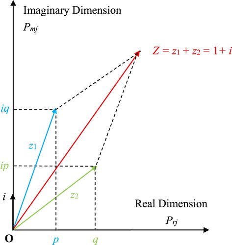
To illustrate the concept of the resultant complex random vector Z, I will use the following graph (Figure 15).

Figure 15. The resultant complex random vector $Z=z_1+z_2$ for a general Bernoulli distribution in the complex probability plane $\mathcal{C}$.

VI.2. The general case: a discrete distribution with N equiprobable random vectors (A uniform distribution U with N random outputs)

As a general case, let us consider then this discrete probability distribution with N equiprobable random vectors which is a discrete uniform probability distribution U with N outputs (Table 2):

Table 2. A discrete uniform distribution with N equiprobable random vectors in $\mathcal{R}$, $\mathcal{M}$, and $\mathcal{C}$.

Outcome	$x_j$	$x_1$	$x_2$	$\dots$	$x_N$
In $\mathcal{R}$	$P_{rj}$	$P_{r1}={\displaystyle \frac{1}{N}}$	$P_{r2}={\displaystyle \frac{1}{N}}$	$\cdots$	$P_{rN}={\displaystyle \frac{1}{N}}$
In $\mathcal{M}$	$P_{mj}$	$P_{m1}=i\left(1-{\displaystyle \frac{1}{N}}\right)$	$P_{m2}=i\left(1-{\displaystyle \frac{1}{N}}\right)$	$\cdots$	$P_{mN}=i\left(1-{\displaystyle \frac{1}{N}}\right)$
In $\mathcal{C}$ = $\mathcal{R}$ + $\mathcal{M}$	$z_j$	$z_1=P_{r1}+{P_m}_1$	$z_2={P_r}_2+{P_m}_2$	$\dots$	$z_N={P_r}_N+{P_m}_N$

We have here in $\mathcal{C}$ = $\mathcal{R}$ + $\mathcal{M}$: $z_j=P_{rj}+P_{mj},\mathrm{\forall }j:1\le j\le N,$ and $z_1=z_2=\dots =z_N=\frac{1}{N}+\frac{i(N-1)}{N}$ $\begin{array}{rl}\Rightarrow Z_U& =\sum _{j=1}^N{z}_j=z_1+z_2+\dots +z_N=N{z}_j\\ & =N\left(\frac{1}{N}+\frac{i(N-1)}{N}\right)=1+i(N-1)\end{array}$ Moreover, we can notice that: $|z_1|=|z_2|=\cdots =|z_N|$, hence, $\begin{array}{rl}|Z_U|& =|z_1+z_2+\dots +z_N|\\ & =N|z_1|=N|z_2|=\dots =N|z_N|\end{array}$ $\begin{array}{rl}\Rightarrow |Z_U{|}^2& =N^2|z_j{|}^2=N^2\left(\frac{1}{N^2}+\frac{{(N-1)}^2}{N^2}\right)\\ & =1+(N-1{)}^2,\text{where}1\le j\le N;\end{array}$ And $\begin{array}{rl}Chf& =N^2\times Ch{f}_j=-2\times {P_r}_j\times \left({P_m}_j/i\right)\times N^2\\ & =-2N^2\times \left(\frac{1}{N}\right)\left(\frac{N-1}{N}\right)=-2\left(1\right)(N-1)\\ & =-2(N-1)\\ & \Rightarrow s^2=|Z_U{|}^2-Chf=1+(N-1{)}^2+2(N-1)\\ & =[1+(N-1){]}^2=N^2\\ \Rightarrow P{c_U}^2& =\frac{s^2}{N^2}=\frac{N^2}{N^2}=1=\frac{{|Z_U|}^2}{N^2}-\frac{Chf}{N^2}\\ & =\frac{1+{(N-1)}^2}{N^2}-\frac{-2(N-1)}{N^2}\\ & =\frac{1+{(N-1)}^2+2(N-1)}{N^2}\\ & =\frac{{[1+(N-1\left)\right]}^2}{N^2}=\frac{N^2}{N^2}=1\\ \Rightarrow P{c}_U& =1\end{array}$ Where s is an intermediary quantity used in our computation of Pc_U.

Therefore, the degree of our knowledge corresponding to the resultant complex vector $Z_U$ representing the whole uniform distribution is: $DO{K}_{Z_U}=\frac{{|Z_U|}^2}{N^2}=\frac{1+{(N-1)}^2}{N^2},$ and its relative chaotic factor is: $Ch{f}_{Z_U}=\frac{Chf}{N^2}=-\frac{2(N-1)}{N^2},$ Similarly, its relative magnitude of the chaotic factor is: $MCh{f}_{Z_U}=|Ch{f}_{Z_U}|=\left|\frac{Chf}{N^2}\right|=\left|-\frac{2(N-1)}{N^2}\right|=\frac{2(N-1)}{N^2}.$ Thus, we can verify that we have always: $\begin{array}{rl}P{c}_U^2& =\frac{{|Z_U|}^2}{N^2}-\frac{Chf}{N^2}=DO{K}_{Z_U}-Ch{f}_{Z_U}\\ & =DO{K}_{Z_U}+MCh{f}_{Z_U}=1\iff P{c}_U=1\end{array}$

What is important here is that we can notice the following fact. Take for example: $\begin{array}{rl}N& =2\Rightarrow DO{K}_{Z_U}=\frac{1+{(2-1)}^2}{2^2}=0.5\text{and}\\ Ch{f}_{Z_U}& =\frac{-2(2-1)}{2^2}=-0.5\end{array}$ $\begin{array}{rl}N& =4\Rightarrow \\ DO{K}_{Z_U}& =\frac{1+{(4-1)}^2}{4^2}=0.625\ge 0.5\text{and}\\ Ch{f}_{Z_U}& =\frac{-2(4-1)}{4^2}=-0.375\ge -0.5\end{array}$ $\begin{array}{rl}N& =5\Rightarrow \\ DO{K}_{Z_U}& =\frac{1+{(5-1)}^2}{5^2}=0.68\ge 0.625\text{and}\\ Ch{f}_{Z_U}& =\frac{-2(5-1)}{5^2}=-0.32\ge -0.375\end{array}$ $\begin{array}{rl}N& =10\Rightarrow \\ DO{K}_{Z_U}& =\frac{1+{(10-1)}^2}{{10}^2}=0.82\ge 0.68\text{and}\\ Ch{f}_{Z_U}& =\frac{-2(10-1)}{{10}^2}=-0.18\ge -0.32\end{array}$ $\begin{array}{rl}N& =100\Rightarrow \\ DO{K}_{Z_U}& =\frac{1+{(100-1)}^2}{{100}^2}=0.9802\ge 0.82\\ \text{and}\\ Ch{f}_{Z_U}& =\frac{-2(100-1)}{{100}^2}=-0.0198\ge -0.18\end{array}$ $\begin{array}{rl}N& =1000\Rightarrow \\ DO{K}_{Z_U}& =\frac{1+{(1000-1)}^2}{{1000}^2}=0.998002\ge 0.9802\text{and}\\ Ch{f}_{Z_U}& =\frac{-2(1000-1)}{{1000}^2}=-0.001998\ge -0.0198\end{array}$

We can deduce mathematically using calculus that: $\begin{array}{rl}\underset{N\to +\mathrm{\infty }}{lim}\frac{{|Z_U|}^2}{N^2}& =\underset{N\to +\mathrm{\infty }}{lim}DO{K}_{Z_U}\\ & =\underset{N\to +\mathrm{\infty }}{lim}\frac{1+{(N-1)}^2}{N^2}=1,\end{array}$ and $\underset{N\to +\mathrm{\infty }}{lim}\frac{Chf}{N^2}=\underset{N\to +\mathrm{\infty }}{lim}Ch{f}_{Z_U}=\underset{N\to +\mathrm{\infty }}{lim}-\frac{2(N-1)}{N^2}=0.$ From the above, we can also deduce this conclusion:

As much as N increases, as much as the degree of our knowledge in $\mathcal{R}$ corresponding to the resultant complex vector is perfect and absolute, that means, it is equal to one, and as much as the chaotic factor that prevents us from foretelling exactly and totally the outcome of the stochastic phenomenon in $\mathcal{R}$ approaches zero. Mathematically we state that: If N tends to infinity then the degree of our knowledge in $\mathcal{R}$ tends to one and the chaotic factor tends to zero.

VI.3. The convergence of Monte Carlo methods using Z and CPP

Subsequently, if $\underset{N\to +\mathrm{\infty }}{lim}Ch{f}_{Z_U}=0$ then $\underset{N\to +\mathrm{\infty }}{lim}Ch{f}_{MC}=0$ (the chaotic factor of Monte Carlo methods) provided that:

1. The Monte Carlo algorithm used to solve the stochastic process or integral is correct

2. The integral that we want to solve using Monte Carlo methods is convergent

Therefore:

1. $\begin{array}{rl}& \Rightarrow \underset{N\to +\mathrm{\infty }}{lim}Ch{f}_{MC}=\underset{N\to +\mathrm{\infty }}{lim}-2P_r{P}_m/i=0\\ & \Rightarrow \left\{\begin{array}{l}{P}_r\to 0\\ \text{OR}\\ P_m/i\to 0\end{array}\right.\Rightarrow \left\{\begin{array}{l}{P}_r\to 0\\ \text{OR}\\ P_r=1-P_m/i\to 1-0=1\end{array}\right.\\ & \Rightarrow \left\{\begin{array}{l}{P}_{\text{rob}}\left(\text{convergence}\right)\to 0\\ \text{OR}\\ P_{\text{rob}}\left(\text{convergence}\right)\to 1\end{array}\right.\end{array}$

   that means either the simulation has not started yet ($P_{rob}(\text{convergence)}=0$) or the Monte Carlo algorithm result or output has converged to the exact result ($P_{rob}(\text{convergence)}\to 1$) since $Ch{f}_{MC}=0$ in only two places which are $N=0$ and $N\to +\mathrm{\infty }$.

2. And $\begin{array}{rl}& \underset{N\to +\mathrm{\infty }}{lim}Ch{f}_{MC}\\ & =\left\{\begin{array}{ll}\begin{array}{l}\underset{N\to +\mathrm{\infty }}{lim}\\ -2\left(\frac{R_A}{R_E}\right)\left(1-\frac{R_A}{R_E}\right)\end{array}& \text{if}0\le R_A\le R_E\\ \begin{array}{l}\underset{N\to +\mathrm{\infty }}{lim}\\ -2\left(2-\frac{R_A}{R_E}\right)\left(\frac{R_A}{R_E}-1\right)\end{array}& \text{if}{R}_E\le R_A\le 2R_E\end{array}\right.\\ & =0\Rightarrow \left\{\begin{array}{l}\frac{R_A}{R_E}\to 0\text{OR}1-\frac{R_A}{R_E}\to 0\\ \text{OR}\\ 2-\frac{R_A}{R_E}\to 0\text{OR}\frac{R_A}{R_E}-1\to 0\end{array}\right.\\ & \Rightarrow \left\{\begin{array}{l}{R}_A\to 0\text{OR}{R}_A\to R_E\\ \text{OR}\\ R_A\to 2R_E\text{OR}{R}_A\to R_E\end{array}\right.\end{array}$

that means either:

• the simulation has not started yet ($R_A=0$ or $R_A=2R_E$) since at this instant the percent relative error is maximum and is equal to 100%,

• or the Monte Carlo algorithm output has converged to the exact result ($R_A\to R_E$) since at this instant the percent relative error is minimum and is equal to 0%,

this is due to the fact that $Ch{f}_{MC}=0$ in only two places which are $N=0$ and $N\to +\mathrm{\infty }$.

Moreover, the speed of the convergence of Monte Carlo methods depends on:

1. The algorithm used

2. The integrand function of the original integral that we want to evaluate ($f\left(x\right)$ or in general $f(x_1,x_2,\dots ,x_n)$) since in Monte Carlo methods: ${\int }_a^{b}f\left(x\right)\text{d}x\cong \frac{b-a}{N}\sum _{j=1}^{N}f\left(x_j\right)$

Or in general: $\begin{array}{rl}& {\int }_{a_1}^{b_1}{\int }_{a_2}^{b_2}\dots {\int }_{a_n}^{b_n}f(x_1,x_2,\dots ,x_n).d{x}_1,d{x}_2\dots d{x}_n\\ & \cong \frac{\left[\right(b_1-a_1)\times (b_2-a_2)\times \dots \times (b_n-a_n\left)\right]}{N}\\ & \times \sum _{j=1}^{N}f(x_{1j},x_{2j},\dots ,x_{nj})\end{array}$

1. The random numbers generator that provides the integrand function with random inputs for the Monte Carlo methods. In the current research work we have used one specific uniform random numbers generator although many others exist in literature.

Furthermore, for $\begin{array}{rl}N& =1\Rightarrow \frac{{|Z|}^2}{N^2}=DO{K}_{Z_U}\\ & =\frac{1+{(1-1)}^2}{1^2}=1\Rightarrow DO{K}_{MC}=1\end{array}$ (the DOK of Monte Carlo methods)

and $\frac{Chf}{N^2}=Ch{f}_{Z_U}=\frac{-2(1-1)}{1^2}=0\Rightarrow Ch{f}_{MC}=0$ This means that we have a random experiment with only one outcome or vector, hence, either $P_r=1$ (always converging) or $P_r=0$ (always diverging), that means we have respectively either a sure event or an impossible event in $\mathcal{R}$. Consequently, we have surely the degree of our knowledge is equal to one (perfect experiment knowledge) and the chaotic factor is equal to zero (no chaos) since the experiment is either certain (that means we have used a deterministic algorithm so the stochastic Monte Carlo methods are replaced by deterministic methods that do not use random numbers like the classical and ordinary methods of numerical integration) or impossible (an incorrect or divergent algorithm or integral), which is absolutely logical.

Consequently, we have proved here the law of large numbers (already discussed in the published paper (Abou Jaoude, 2015b)) as well as the convergence of Monte Carlo methods using CPP. The following figures (Figures 16 and 17) show the convergence of $Ch{f}_{Z_U}$ to 0 and of $DO{K}_{Z_U}$ to 1 as functions of the uniform samples number N (Number of inputs/outputs).

Figure 16. $Ch{f}_{Z_U}$,$DO{K}_{Z_U}$, and $P{c}_U$, as functions of N in 2D.

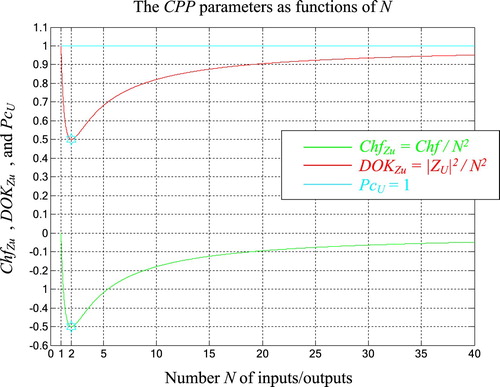
Figure 17. $Ch{f}_{Z_U}$,$DO{K}_{Z_U}$, and $P{c}_U$, as functions of N in 3D.

VII. The Evaluation of the new paradigm parameters

We can deduce from what has been elaborated previously the following:

The real convergence probability: $P_r\left(N\right)=1-\left|\frac{R_E-R_A\left(N\right)}{R_E}\right|$ We have $0\le N\le N_C$ where N = 0 corresponds to the instant before the beginning of the random experiment when $R_A(N=0)=0\text{ or }=2R_E$, and $N=N_C$ (iterations number needed for the method convergence) corresponds to the instant at the end of the random experiments and Monte Carlo methods when $R_A(N=N_C)\to R_E$.

The imaginary divergence probability: $P_m\left(N\right)=i\left|\frac{R_E-R_A\left(N\right)}{R_E}\right|$ The real complementary divergence probability: $P_m\left(N\right)/i=\left|\frac{R_E-R_A\left(N\right)}{R_E}\right|$

The complex probability and random vector: $\begin{array}{rl}Z\left(N\right)& =P_r\left(N\right)+P_m\left(N\right)\\ & =\left[1-\left|\frac{R_E-R_A\left(N\right)}{R_E}\right|\right]+i\left|\frac{R_E-R_A\left(N\right)}{R_E}\right|\end{array}$ The Degree of Our Knowledge: $\begin{array}{rl}DOK\left(N\right)& =|Z\left(N\right){|}^2=P_r^2\left(N\right)+[P_m\left(N\right)/i{]}^2\\ & ={\left[1-\left|\frac{R_E-R_A\left(N\right)}{R_E}\right|\right]}^2+{\left[\left|\frac{R_E-R_A\left(N\right)}{R_E}\right|\right]}^2\\ & =1+2i{P}_r\left(N\right)P_m\left(N\right)=1-2P_r\left(N\right)\left[1-P_r\left(N\right)\right]\\ & =1-2P_r\left(N\right)+2P_r^2\left(N\right)\\ & =1-2\left|\frac{R_E-R_A\left(N\right)}{R_E}\right|+2{\left[\frac{R_E-R_A\left(N\right)}{R_E}\right]}^2\end{array}$ The Chaotic Factor: $\begin{array}{rl}Chf\left(N\right)& =2i{P}_r\left(N\right)P_m\left(N\right)=-2P_r\left(N\right)\left[1-P_r\left(N\right)\right]\\ & =-2P_r\left(N\right)+2P_r^2\left(N\right)\\ & =-2\left|\frac{R_E-R_A\left(N\right)}{R_E}\right|+2{\left[\frac{R_E-R_A\left(N\right)}{R_E}\right]}^2\end{array}$ $Chf\left(N\right)$ is null when $P_r\left(N\right)=P_r\left(0\right)=0$ and when $P_r\left(N\right)=P_r\left(N_C\right)=1$.

The Magnitude of the Chaotic Factor MChf: $\begin{array}{rl}MChf\left(N\right)& =|Chf\left(N\right)|=-2i{P}_r\left(N\right)P_m\left(N\right)\\ & =2P_r\left(N\right)\left[1-P_r\left(N\right)\right]=2P_r\left(N\right)-2P_r^2\left(N\right)\\ & =2\left|\frac{R_E-R_A\left(N\right)}{R_E}\right|-2{\left[\frac{R_E-R_A\left(N\right)}{R_E}\right]}^2\end{array}$ $MChf\left(N\right)$ is null when $P_r\left(N\right)=P_r\left(0\right)=0$ and when $P_r\left(N\right)=P_r\left(N_C\right)=1$.

At any iteration number N: $0\le \mathrm{\forall }N\le N_C$, the probability expressed in the complex probability set $\mathcal{C}$ is the following: $\begin{array}{rl}P{c}^2\left(N\right)& =\left[P_r\right(N)+P_m(N)/i{]}^2=|Z\left(N\right){|}^2-2i{P}_r\left(N\right)P_m\left(N\right)\\ & =DOK\left(N\right)-Chf\left(N\right)\\ & =DOK\left(N\right)+MChf\left(N\right)\\ & =1\end{array}$ then, $P{c}^2\left(N\right)=\left[P_r\right(N)+P_m(N)/i{]}^2=\left\{P_r\right(N)+[1-P_r\left(N\right)]{\}}^2=1^2\iff Pc=1$ always

Hence, the prediction of the convergence probabilities of the stochastic Monte Carlo experiments in the set $\mathcal{C}$ is permanently certain.

Let us consider thereafter some stochastic experiments and some single and multidimensional integrals to simulate the Monte Carlo methods and to draw, to visualize, as well as to quantify all the CPP and prognostic parameters.

VIII. Flowchart of the complex probability and Monte Carlo methods prognostic model

The following flowchart summarizes all the procedures of the proposed complex probability prognostic model:

IX. Simulation of the new paradigm

Note that all the numerical values found in the simulations of the new paradigm for any iteration cycles N were computed using the MATLAB version 2019 software. In addition, the reader should take care of the rounding errors since all numerical values are represented by at most five significant digits and since we are using Monte Carlo methods of integration and simulation which give approximate results subject to random effects and fluctuations.

IX.1. The continuous random case

IX.1.1. The first simple integral: a linear function

Let us consider the integral of the following linear function: ${\int }_0^{1}x\text{d}x={\left[\frac{x^2}{2}\right]}_0^1=\frac{1^2}{2}-0=\frac{1}{2}=0.5\iff R_E=0.5$ by the deterministic methods of calculus. $\iff f\left(x\right)=x,x\mapsto U(0,1)$ $\iff {\int }_0^{1}x\text{d}x\cong \frac{1}{N}\sum _{j=1}^N{x}_j=R_A$ with $1\le N\le N_C$ after applying Monte Carlo method.

Moreover, the four figures (Figures 18–21) show the increasing convergence of Monte Carlo method and simulation to the exact result $R_E=0.5$ for N = 50, 100, 500, and $N=N_C=100,000$ iterations. Therefore, we have: $\begin{array}{rl}\underset{N\to +\mathrm{\infty }}{lim}{P}_r\left(N\right)& =\underset{N\to +\mathrm{\infty }}{lim}\left\{1-\left|\frac{R_E-R_A\left(N\right)}{R_E}\right|\right\}\\ & =1-\left|\frac{R_E-R_E}{R_E}\right|=1-0=1\end{array}$ which is equal to the convergence probability of Monte Carlo method as $N\to +\mathrm{\infty }$.

Figure 18. The increasing convergence of the Monte Carlo method up to N = 50 iterations.

Figure 19. The increasing convergence of the Monte Carlo method up to N = 100 iterations.

Figure 20. The increasing convergence of the Monte Carlo method up to N = 500 iterations.

Figure 21. The increasing convergence of the Monte Carlo method up to N = 100,000 iterations.

Additionally, Figure 22 illustrates clearly and visibly the relation of Monte Carlo method to the complex probability paradigm with all its parameters ($Chf,R_A,P_r,MChf,R_E,DOK,P_m/i,Pc$) after applying it to this linear function.

Figure 22. The CPP parameters and the Monte Carlo method for a linear function.

IX.1.2. The second simple integral: a cubic function

Let us consider the integral of the following cubic function: ${\int }_0^1{x}^3\text{d}x={\left[\frac{x^4}{4}\right]}_0^1=\frac{1^4}{4}-0=\frac{1}{4}=0.25\iff R_E=0.25$ by the deterministic methods of calculus. $\begin{array}{r}\iff f\left(x\right)=x^3,x\mapsto U(0,1)\\ \iff {\int }_0^1{x}^3\text{d}x\cong \frac{1}{N}\sum _{j=1}^N{x}_j^3=R_A\end{array}$ with $1\le N\le N_C$ after applying Monte Carlo method.

Moreover, the four figures (Figures 23–26) show the increasing convergence of Monte Carlo method and simulation to the exact result $R_E=0.25$ for N = 50, 100, 500, and $N=N_C=100,000$ iterations. Therefore, we have: $\begin{array}{rl}\underset{N\to +\mathrm{\infty }}{lim}{P}_r\left(N\right)& =\underset{N\to +\mathrm{\infty }}{lim}\left\{1-\left|\frac{R_E-R_A\left(N\right)}{R_E}\right|\right\}\\ & =1-\left|\frac{R_E-R_E}{R_E}\right|=1-0=1\end{array}$

Figure 23. The increasing convergence of the Monte Carlo method up to N = 50 iterations.

Figure 24. The increasing convergence of the Monte Carlo method up to N = 100 iterations.

Figure 25. The increasing convergence of the Monte Carlo method up to N = 500 iterations.

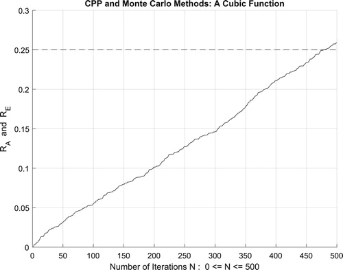
Figure 26. The increasing convergence of the Monte Carlo method up to N = 100,000 iterations.

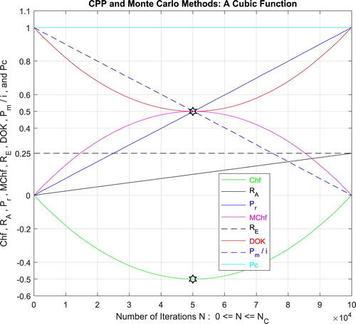
which is equal to the convergence probability of Monte Carlo method as $N\to +\mathrm{\infty }$. Additionally, Figure 27 illustrates clearly and visibly the relation of Monte Carlo method to the complex probability paradigm with all its parameters ($Chf,R_A,P_r,MChf,R_E,DOK,P_m/i,Pc$) after applying it to this cubic function.

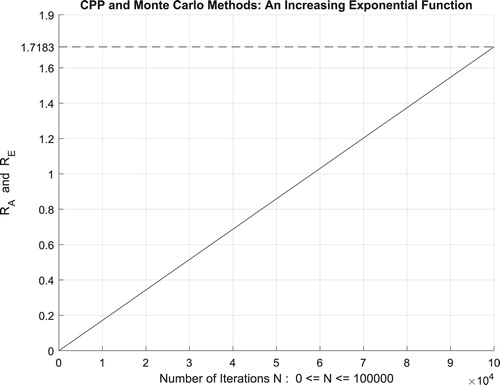
IX.1.3. The third simple integral: an increasing exponential function

Let us consider the integral of the following increasing exponential function: $\begin{array}{rl}{\int }_0^1\exp \left(x\right)\text{d}x& =[\exp \left(x\right){]}_0^1=\exp (1)-\exp (0)\\ & =e-1=2.718281828\dots -1\\ & =1.718281828\dots \\ \iff R_E& =1.718281828\dots \end{array}$ by the deterministic methods of calculus. $\begin{array}{rl}\iff f\left(x\right)& =\exp \left(x\right),x\mapsto U(0,1)\\ \iff {\int }_0^1\exp \left(x\right)\text{d}x& \cong \frac{1}{N}\sum _{j=1}^N\exp \left(x_j\right)=R_A\end{array}$ with $1\le N\le N_C$ after applying Monte Carlo method.

Figure 27. The CPP parameters and the Monte Carlo method for a cubic function.

Moreover, the four figures (Figures 28–31) show the increasing convergence of Monte Carlo method and simulation to the exact result $R_E=1.718281828\dots$ for N = 50, 100, 500, and $N=N_C=100,000$ iterations. Therefore, we have: $\begin{array}{rl}\underset{N\to +\mathrm{\infty }}{lim}{P}_r\left(N\right)& =\underset{N\to +\mathrm{\infty }}{lim}\left\{1-\left|\frac{R_E-R_A\left(N\right)}{R_E}\right|\right\}\\ & =1-\left|\frac{R_E-R_E}{R_E}\right|=1-0=1\end{array}$ which is equal to the convergence probability of Monte Carlo method as $N\to +\mathrm{\infty }$.

Figure 28. The increasing convergence of the Monte Carlo method up to N = 50 iterations.

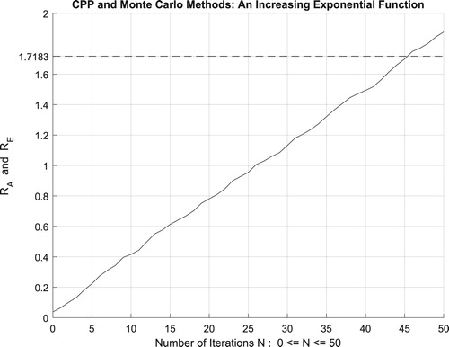
Figure 29. The increasing convergence of the Monte Carlo method up to N = 100 iterations.

Figure 30. The increasing convergence of the Monte Carlo method up to N = 500 iterations.

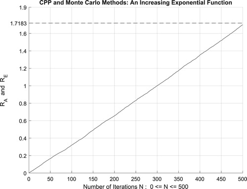
Figure 31. The increasing convergence of the Monte Carlo method up to N = 100,000 iterations.

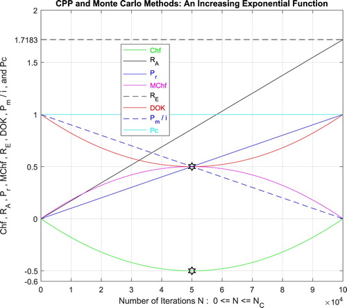
Additionally, Figure 32 illustrates clearly and visibly the relation of Monte Carlo method to the complex probability paradigm with all its parameters ($Chf,R_A,P_r,MChf,R_E,DOK,P_m/i,Pc$) after applying it to this increasing exponential function.

Figure 32. The CPP parameters and the Monte Carlo method for an increasing exponential function.

IX.1.4. The fourth simple integral: a logarithmic function

Let us consider the integral of the following logarithmic function: $\begin{array}{rl}& {\int }_1^{2}Ln\left(x\right)\text{d}x=[xLn\left(x\right)-x{]}_1^2=2Ln2-1\\ & =0.386294361\dots \iff R_E=0.386294361\dots \end{array}$ by the deterministic methods of calculus. $\begin{array}{rl}\iff f\left(x\right)& =Ln\left(x\right),x\mapsto U(1,2)\\ \iff {\int }_1^{2}Ln\left(x\right)\text{d}x& \cong \frac{(2-1)}{N}\sum _{j=1}^{N}Ln\left(x_j\right)\\ & =\frac{1}{N}\sum _{j=1}^{N}Ln\left(x_j\right)=R_A\end{array}$ with $1\le N\le N_C$ after applying Monte Carlo method.

Moreover, the four figures (Figures 33–36) show the increasing convergence of Monte Carlo method and simulation to the exact result $R_E=0.386294361\dots$ for N = 50, 100, 500, and $N=N_C=100,000$ iterations. Therefore, we have: $\begin{array}{rl}\underset{N\to +\mathrm{\infty }}{lim}{P}_r\left(N\right)& =\underset{N\to +\mathrm{\infty }}{lim}\left\{1-\left|\frac{R_E-R_A\left(N\right)}{R_E}\right|\right\}\\ & =1-\left|\frac{R_E-R_E}{R_E}\right|=1-0=1\end{array}$ which is equal to the convergence probability of Monte Carlo method as $N\to +\mathrm{\infty }$. Additionally, Figure 37 illustrates clearly and visibly the relation of Monte Carlo method to the complex probability paradigm with all its parameters ($Chf,R_A,P_r,MChf,R_E,DOK,P_m/i,Pc$) after applying it to this logarithmic function.

Figure 33. The increasing convergence of the Monte Carlo method up to N = 50 iterations.

Figure 34. The increasing convergence of the Monte Carlo method up to N = 100 iterations.

Figure 35. The increasing convergence of the Monte Carlo method up to N = 500 iterations.

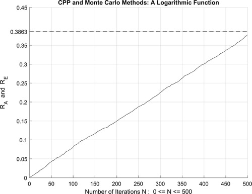
Figure 36. The increasing convergence of the Monte Carlo method up to N = 100,000 iterations.

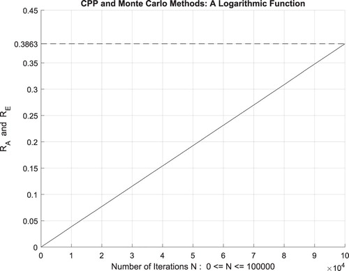
Figure 37. The CPP parameters and the Monte Carlo method for a logarithmic function.

IX.1.5. A multiple integral

Let us consider the multidimensional integral of the following function: $\begin{array}{rl}& {\int }_0^{3/2}{\int }_0^{3/2}{\int }_0^{3/2}xyz.\text{d}x\text{d}y\text{d}z\\ & ={\int }_0^{3/2}{\int }_0^{3/2}{\left[\frac{x^2}{2}\right]}_0^{3/2}yz.\text{d}y\text{d}z\\ & ={\int }_0^{3/2}{\int }_0^{3/2}\frac{9}{8}yz.\text{d}y\text{d}z=\frac{9}{8}{\int }_0^{3/2}{\left[\frac{y^2}{2}\right]}_0^{3/2}z.dz\\ & =\frac{9}{8}{\int }_0^{3/2}\frac{9}{8}z.\text{d}z\\ & =\frac{81}{64}{\left[\frac{z^2}{2}\right]}_0^{3/2}=\frac{81}{64}\times \frac{9}{8}\\ & =\frac{729}{512}=1.423828125\dots \iff R_E=1.423828125\dots \end{array}$ by the deterministic methods of calculus. $\begin{array}{rl}& \iff f(x,y,z)=xyz,x\mapsto U(0,3/2),y\mapsto U(0,3/2),\\ z& \mapsto U(0,3/2)\\ & \iff {\int }_0^{3/2}{\int }_0^{3/2}{\int }_0^{3/2}xyz.\text{d}x\text{d}y\text{d}z\\ & \cong \frac{\left[\right(3/2-0)\times (3/2-0)\times (3/2-0\left)\right]}{N}\sum _{j=1}^N{x}_j{y}_j{z}_j\\ & =\frac{27/8}{N}\sum _{j=1}^N{x}_j{y}_j{z}_j=R_A\end{array}$ with $1\le N\le N_C$ after applying Monte Carlo method.

Moreover, the four figures (Figures 38–41) show the increasing convergence of Monte Carlo method and simulation to the exact result $R_E=1.423828125\dots$ for N = 50, 100, 500, and $N=N_C=100,000$ iterations. Therefore, we have: $\begin{array}{rl}\underset{N\to +\mathrm{\infty }}{lim}{P}_r\left(N\right)& =\underset{N\to +\mathrm{\infty }}{lim}\left\{1-\left|\frac{R_E-R_A\left(N\right)}{R_E}\right|\right\}\\ & =1-\left|\frac{R_E-R_E}{R_E}\right|=1-0=1\end{array}$ which is equal to the convergence probability of Monte Carlo method as $N\to +\mathrm{\infty }$.

Additionally, Figure 42 illustrates clearly and visibly the relation of Monte Carlo method to the complex probability paradigm with all its parameters ($Chf,R_A,P_r,MChf,R_E,DOK,P_m\text{/}i,Pc$) after applying it to this three-dimensional integral.

Figure 38. The increasing convergence of the Monte Carlo method up to N = 50 iterations.

Figure 39. The increasing convergence of the Monte Carlo method up to N = 100 iterations.

Figure 40. The increasing convergence of the Monte Carlo method up to N = 500 iterations.

Figure 41. The increasing convergence of the Monte Carlo method up to N = 100,000 iterations.

Figure 42. The CPP parameters and the Monte Carlo method for a multiple integral.

IX.2. The discrete random case

IX.2.1. The first random experiment: a random walk in a plane

We will try in this problem to simulate random walks in a plane, each walk starting at O(0,0) and consisting of s = 10000 steps of length = L = 0.008. The probability theory says that after s steps, the expected distance from the starting point will be $L\times \sqrt{s}$. So, the estimated distance in the programme will be $=0.008\times \sqrt{10000}=0.008\times 100=0.8=R_E$. The figure below shows a random walk in a plane (Figure 43):

Figure 43. A random walk simulation in a plane.

Moreover, the four figures (Figures 44–47) show the increasing convergence of Monte Carlo method and simulation to the exact result $R_E=0.8$ for N = 50, 100, 500, and $N=N_C=100,000$ iterations. Therefore, we have: $\begin{array}{rl}\underset{N\to +\mathrm{\infty }}{lim}{P}_r\left(N\right)& =\underset{N\to +\mathrm{\infty }}{lim}\left\{1-\left|\frac{R_E-R_A\left(N\right)}{R_E}\right|\right\}\\ & =1-\left|\frac{R_E-R_E}{R_E}\right|=1-0=1\end{array}$ which is equal to the convergence probability of Monte Carlo method as $N\to +\mathrm{\infty }$.

Additionally, Figure 48 illustrates clearly and visibly the relation of Monte Carlo method to the complex probability paradigm with all its parameters ($Chf,R_A,P_r,MChf,R_E,DOK,P_m/i,Pc$) after applying it to this random walk problem.

Figure 44. The increasing convergence of the Monte Carlo method up to N = 50 iterations.

Figure 45. The increasing convergence of the Monte Carlo method up to N = 100 iterations.

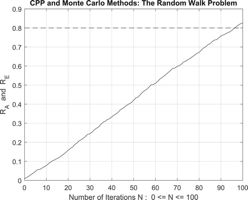
Figure 46. The increasing convergence of the Monte Carlo method up to N = 500 iterations.

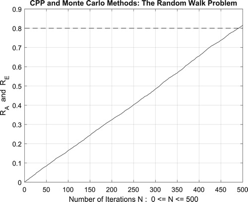
Figure 47. The increasing convergence of the Monte Carlo method up to N = 100,000 iterations.

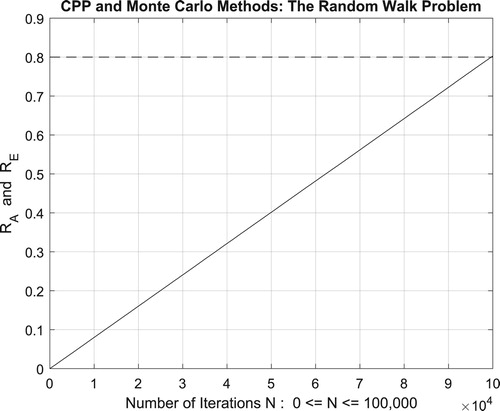
Figure 48. The CPP parameters and the Monte Carlo method for the random walk problem.

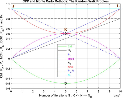
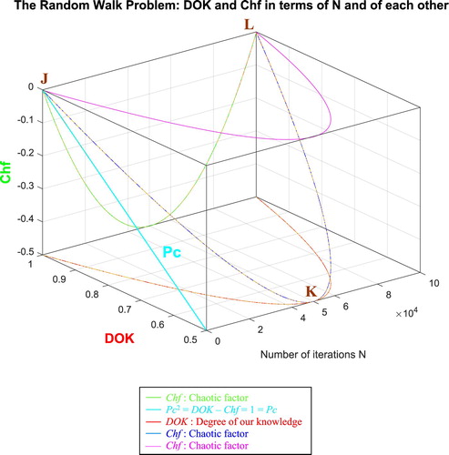
IX.2.1.1. The complex probability cubes

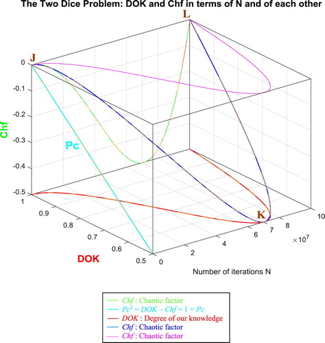
In the first cube (Figure 49), the simulation of DOK and Chf as functions of each other and of the iterations N for the random walk problem can be seen. The line in cyan is the projection of Pc²(N) = DOK(N) - Chf(N) = 1 = Pc(N) on the plane N = 0 iterations. This line starts at the point J (DOK = 1, Chf = 0) when N = 0 iterations, reaches the point (DOK = 0.5, Chf = −0.5) when N = 50,000 iterations, and returns at the end to J (DOK = 1, Chf = 0) when N = N_C = 100,000 iterations. The other curves are the graphs of DOK(N) (red) and Chf(N) (green, blue, pink) in different planes. Notice that they all have a minimum at the point K (DOK = 0.5, Chf = −0.5, N = 50,0000 iterations). The point L corresponds to (DOK = 1, Chf = 0, N = N_C = 100,000 iterations). The three points J, K, L are the same as in Figure 48.

Figure 49. DOK and Chf in terms of N and of each other for the random walk problem.

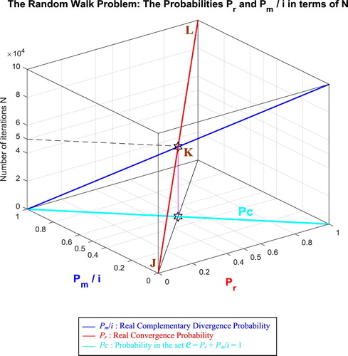
In the second cube (Figure 50), we can notice the simulation of the convergence probability P_r(N) and its complementary real divergence probability P_m(N)/i in terms of the iterations N for the random walk problem. The line in cyan is the projection of Pc²(N) = P_r(N) + P_m(N)/i = 1 = Pc(N) on the plane N = 0 iterations. This line starts at the point (P_r = 0, P_m/i = 1) and ends at the point (P_r = 1, P_m/i = 0). The red curve represents P_r(N) in the plane P_r(N) = P_m(N)/i. This curve starts at the point J (P_r = 0, P_m/i = 1, N = 0 iterations), reaches the point K (P_r = 0.5, P_m/i = 0.5, N = 50,000 iterations), and gets at the end to L (P_r = 1, P_m/i = 0, N = N_C = 100,000 iterations). The blue curve represents P_m(N)/i in the plane P_r(N) + P_m(N)/i = 1. Notice the importance of the point K which is the intersection of the red and blue curves at N = 50,000 iterations and when P_r(N) = P_m(N)/i = 0.5. The three points J, K, L are the same as in Figure 48.

Figure 50. P_r and P_m/i in terms of N and of each other for the random walk problem.

In the third cube (Figure 51), we can notice the simulation of the complex random vector Z(N) in $\mathcal{C}$ as a function of the real convergence probability P_r(N) = Re(Z) in $\mathcal{R}$ and of its complementary imaginary divergence probability P_m(N) = i × Im(Z) in $\mathcal{M}$, and this in terms of the iterations N for the random walk problem. The red curve represents P_r(N) in the plane P_m(N) = 0 and the blue curve represents P_m(N) in the plane P_r(N) = 0. The green curve represents the complex probability vector Z(N) = P_r(N) + P_m(N) = Re(Z) + i × Im(Z) in the plane P_r(N) = iP_m(N) + 1. The curve of Z(N) starts at the point J (P_r = 0, P_m = i, N = 0 iterations) and ends at the point L (P_r = 1, P_m = 0, N = N_C = 100,000 iterations). The line in cyan is P_r(0) = iP_m(0) + 1 and it is the projection of the Z(N) curve on the complex probability plane whose equation is N = 0 iterations. This projected line starts at the point J (P_r = 0, P_m = i, N = 0 iterations) and ends at the point (P_r = 1, P_m = 0, N = 0 iterations). Notice the importance of the point K corresponding to N = 50,000 iterations and when P_r = 0.5 and P_m = 0.5i. The three points J, K, L are the same as in Figure 48.

Figure 51. The Complex Probability Vector Z in terms of N for the random walk problem.

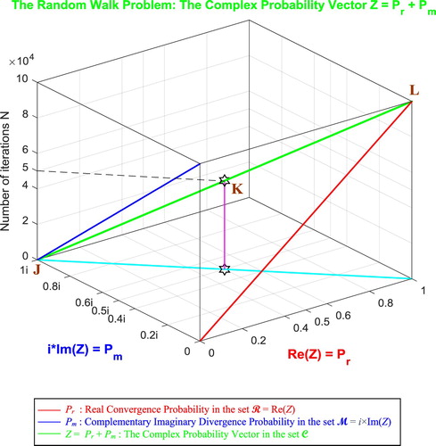
Figure 52. The increasing convergence of the Monte Carlo method up to N = 50 iterations.

IX.2.2. The second random experiment: the birthday problem

The given of the second random experiment is the following: Find the probability that n people $(n\le 365)$ selected at random will have n different birthdays.

Theoretical Analysis

We assume that there are only 365 days in a year (not a leap year) and that all birthdays are equally probable, assumptions which are not quite met in reality.

The first of the n people has of course some birthday with probability 365/365 = 1. Then, if the second is to have a different birthday, it must occur on one of the other days. Therefore, the probability that the second person has a birthday different from the first is 364/365. Similarly, the probability that the third person has a birthday different from the first two is 363/365. Finally, the probability that the nth person has a birthday different from the others is $(365-n+1)/365$. We therefore have: $\begin{array}{rl}& P\left(\text{all}n\text{birthdays}\text{are}\text{different}\right)=\frac{365}{365}\times \frac{364}{365}\times \frac{363}{365}\\ & \times \dots \times \left(1-\frac{n-1}{365}\right)=R_E\end{array}$ The table below gives the theoretical probabilities of different birthdays for a selected number of people n (Table 3).

Table 3. The theoretical probabilities of distinct birthdays for n people where n ≥ 1.

Number of People n	Theoretical Probability = RE
n = 1	P = 1
n = 2	P = 0.99726
n = 3	P = 0.991796
n = 4	P = 0.983644
n = 5	P = 0.972864
n = 10	P = 0.883052
n = 20	P = 0.588562
n = 50	P = 0.0296264
n = 75	P = 0.000280122
n = 100	P = 0.000000307249
n > 365	P = 0

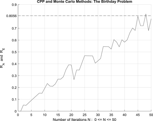
Moreover, the four figures (Figures 52–55) show the increasing convergence of Monte Carlo method and simulation to the exact result $R_E=0.80558972\dots$ for $n=13$ people and for N = 50, 100, 500, and $N=N_C=500,000,000$ iterations. Therefore, we have: $\begin{array}{rl}\underset{N\to +\mathrm{\infty }}{lim}{P}_r\left(N\right)& =\underset{N\to +\mathrm{\infty }}{lim}\left\{1-\left|\frac{R_E-R_A\left(N\right)}{R_E}\right|\right\}\\ & =1-\left|\frac{R_E-R_E}{R_E}\right|=1-0=1\end{array}$ which is equal to the convergence probability of Monte Carlo method as $N\to +\mathrm{\infty }$.

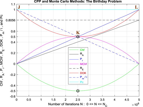
Additionally, Figure 56 illustrates clearly and visibly the relation of Monte Carlo method to the complex probability paradigm with all its parameters ($Chf,R_A,P_r,MChf,R_E,DOK,P_m/i,Pc$) after applying it to this birthday problem.

Figure 53. The increasing convergence of the Monte Carlo method up to N = 100 iterations.

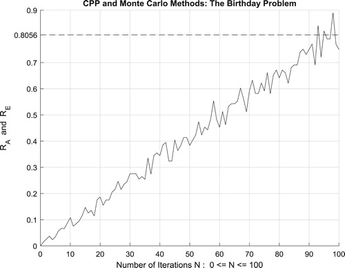
Figure 54. The increasing convergence of the Monte Carlo method up to N = 500 iterations.

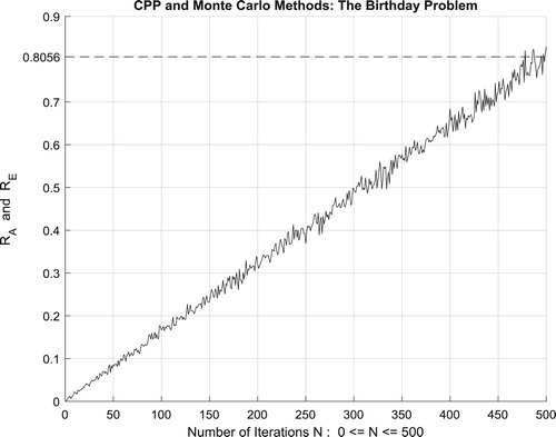
Figure 55. The increasing convergence of the Monte Carlo method up to N = 500,000,000 iterations.

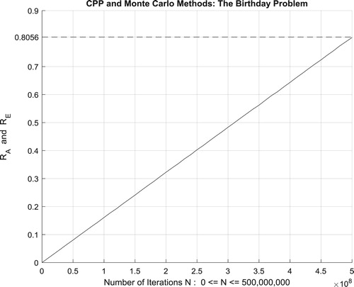
Figure 56. The CPP parameters and the Monte Carlo method for the birthday problem.

IX.2.2.1. The complex probability cubes

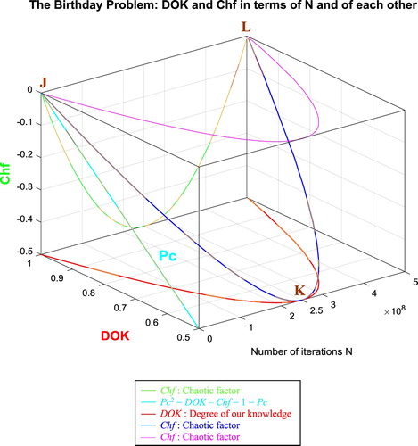
In the first cube (Figure 57), the simulation of DOK and Chf as functions of each other and of the iterations N for the birthday problem can be seen. The line in cyan is the projection of Pc²(N) = DOK(N) - Chf(N) = 1 = Pc(N) on the plane N = 0 iterations. This line starts at the point J (DOK = 1, Chf = 0) when N = 0 iterations, reaches the point (DOK = 0.5, Chf = −0.5) when N = 250,000,000 iterations, and returns at the end to J (DOK = 1, Chf = 0) when N = N_C = 500,000,000 iterations. The other curves are the graphs of DOK(N) (red) and Chf(N) (green, blue, pink) in different planes. Notice that they all have a minimum at the point K (DOK = 0.5, Chf = −0.5, N = 250,000,000 iterations). The point L corresponds to (DOK = 1, Chf = 0, N = N_C = 500,000,000 iterations). The three points J, K, L are the same as in Figure 56.

Figure 57. DOK and Chf in terms of N and of each other for the birthday problem.

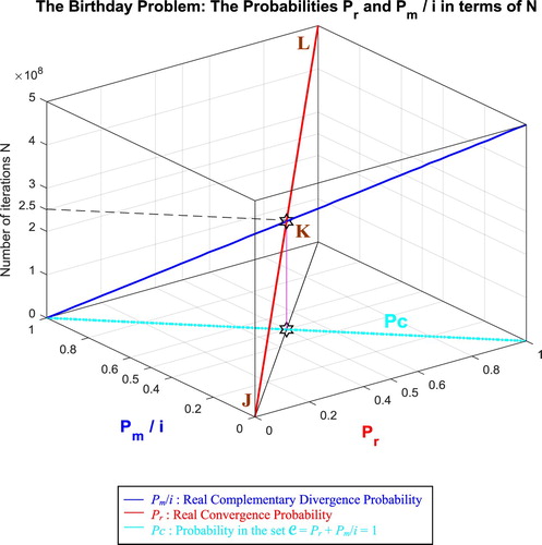
In the second cube (Figure 58), we can notice the simulation of the convergence probability P_r(N) and its complementary real divergence probability P_m(N)/i in terms of the iterations N for the birthday problem. The line in cyan is the projection of Pc²(N) = P_r(N) + P_m(N)/i = 1 = Pc(N) on the plane N = 0 iterations. This line starts at the point (P_r = 0, P_m/i = 1) and ends at the point (P_r = 1, P_m/i = 0). The red curve represents P_r(N) in the plane P_r(N) = P_m(N)/i. This curve starts at the point J (P_r = 0, P_m/i = 1, N = 0 iterations), reaches the point K (P_r = 0.5, P_m/i = 0.5, N = 250,000,000 iterations), and gets at the end to L (P_r = 1, P_m/i = 0, N = N_C = 500,000,000 iterations). The blue curve represents P_m(N)/i in the plane P_r(N) + P_m(N)/i = 1. Notice the importance of the point K which is the intersection of the red and blue curves at N = 250,000,000 iterations and when P_r(N) = P_m(N)/i = 0.5. The three points J, K, L are the same as in Figure 56.

Figure 58. P_r and P_m/i in terms of N and of each other for the birthday problem.

In the third cube (Figure 59), we can notice the simulation of the complex random vector Z(N) in $\mathcal{C}$ as a function of the real convergence probability P_r(N) = Re(Z) in $\mathcal{R}$ and of its complementary imaginary divergence probability P_m(N) = i × Im(Z) in $\mathcal{M}$, and this in terms of the iterations N for the birthday problem. The red curve represents P_r(N) in the plane P_m(N) = 0 and the blue curve represents P_m(N) in the plane P_r(N) = 0. The green curve represents the complex probability vector Z(N) = P_r(N) + P_m(N) = Re(Z) + i × Im(Z) in the plane P_r(N) = iP_m(N) + 1. The curve of Z(N) starts at the point J (P_r = 0, P_m = i, N = 0 iterations) and ends at the point L (P_r = 1, P_m = 0, N = N_C = 500,000,000 iterations). The line in cyan is P_r(0) = iP_m(0) + 1 and it is the projection of the Z(N) curve on the complex probability plane whose equation is N = 0 iterations. This projected line starts at the point J (P_r = 0, P_m = i, N = 0 iterations) and ends at the point (P_r = 1, P_m = 0, N = 0 iterations). Notice the importance of the point K corresponding to N = 250,000,000 iterations and when P_r = 0.5 and P_m = 0.5i. The three points J, K, L are the same as in Figure 56.

Figure 59. The Complex Probability Vector Z in terms of N for the birthday problem.

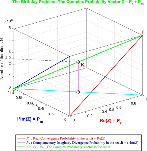
Figure 60. The increasing convergence of the Monte Carlo method up to N = 50 iterations.

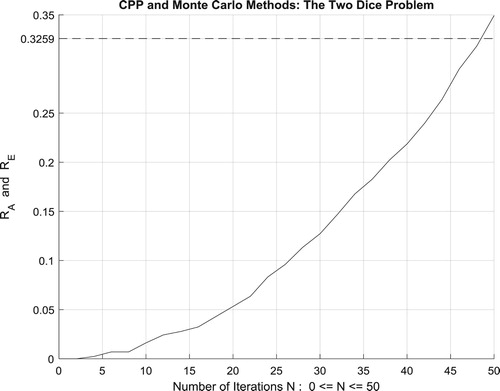
IX.2.3. The third random experiment: the two dice problem

The following programme has an analytic solution beside a simulated solution. This is advantageous for us because we wish to compare the results of Monte Carlo simulations with theoretical solutions. Consider the experiment of tossing two dice. For an unloaded die, the numbers 1,2,3,4,5, and 6 are equally likely to occur. We ask: What is the probability of throwing a 12 (i.e. 6 appearing on each die) in 14 throws of the dice?

There are six possible outcomes from each die for a total of 36 possible combinations. Only one of these combinations is a double 6, so 35 out of the 36 combinations are not correct. With 14 throws, we have $(35/36{)}^{14}$ as the probability of a wrong outcome. Hence, $1-(35/36{)}^{14}=0.325910425\dots$ is the exact answer and therefore the value of $R_E$. Not all random problems of this type can be analyzed like this.

Moreover, the four figures (Figures 60–63) show the increasing convergence of Monte Carlo method and simulation to the exact result $R_E=0.325910425\dots$ for N = 50, 100, 500, and $N=N_C=100,000,000$ iterations. Therefore, we have: $\begin{array}{rl}\underset{N\to +\mathrm{\infty }}{lim}{P}_r\left(N\right)& =\underset{N\to +\mathrm{\infty }}{lim}\left\{1-\left|\frac{R_E-R_A\left(N\right)}{R_E}\right|\right\}\\ & =1-\left|\frac{R_E-R_E}{R_E}\right|=1-0=1\end{array}$ which is equal to the convergence probability of Monte Carlo method as $N\to +\mathrm{\infty }$.

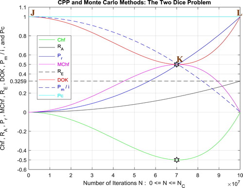
Additionally, Figure 64 illustrates clearly and visibly the relation of Monte Carlo method to the complex probability paradigm with all its parameters ($Chf,R_A,P_r,MChf,R_E,DOK,P_m/i,Pc$) after applying it to this two dice problem.

Figure 61. The increasing convergence of the Monte Carlo method up to N = 100 iterations.

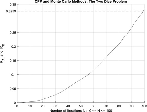
Figure 62. The increasing convergence of the Monte Carlo method up to N = 500 iterations.

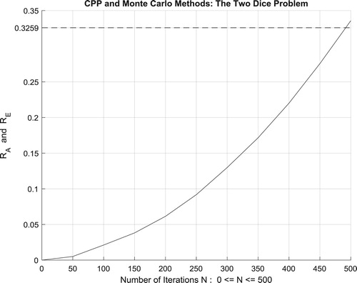
Figure 63. The increasing convergence of the Monte Carlo method up to N = 100,000,000 iterations.

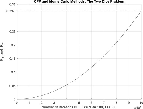
Figure 64. The CPP parameters and the Monte Carlo method for the two dice problem.

IX.2.3.1. The complex probability cubes

In the first cube (Figure 65), the simulation of DOK and Chf as functions of each other and of the iterations N for the two dice problem can be seen. The line in cyan is the projection of Pc²(N) = DOK(N) - Chf(N) = 1 = Pc(N) on the plane N = 0 iterations. This line starts at the point J (DOK = 1, Chf = 0) when N = 0 iterations, reaches the point (DOK = 0.5, Chf = −0.5) when N = 70,000,000 iterations, and returns at the end to J (DOK = 1, Chf = 0) when N = N_C = 100,000,000 iterations. The other curves are the graphs of DOK(N) (red) and Chf(N) (green, blue, pink) in different planes. Notice that they all have a minimum at the point K (DOK = 0.5, Chf = −0.5, N = 70,000,000 iterations). The point L corresponds to (DOK = 1, Chf = 0, N = N_C = 100,000,000 iterations). The three points J, K, L are the same as in Figure 64.

Figure 65. DOK and Chf in terms of N and of each other for the two dice problem.

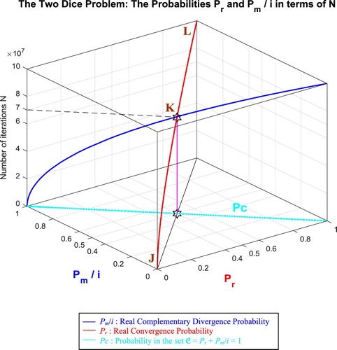
In the second cube (Figure 66), we can notice the simulation of the convergence probability P_r(N) and its complementary real divergence probability P_m(N)/i in terms of the iterations N for the two dice problem. The line in cyan is the projection of Pc²(N) = P_r(N) + P_m(N)/i = 1 = Pc(N) on the plane N = 0 iterations. This line starts at the point (P_r = 0, P_m/i = 1) and ends at the point (P_r = 1, P_m/i = 0). The red curve represents P_r(N) in the plane P_r(N) = P_m(N)/i. This curve starts at the point J (P_r = 0, P_m/i = 1, N = 0 iterations), reaches the point K (P_r = 0.5, P_m/i = 0.5, N = 70,000,000 iterations), and gets at the end to L (P_r = 1, P_m/i = 0, N = N_C = 100,000,000 iterations). The blue curve represents P_m(N)/i in the plane P_r(N) + P_m(N)/i = 1. Notice the importance of the point K which is the intersection of the red and blue curves at N = 70,000,000 iterations and when P_r(N) = P_m(N)/i = 0.5. The three points J, K, L are the same as in Figure 64.

Figure 66. P_r and P_m/i in terms of N and of each other for the two dice problem.

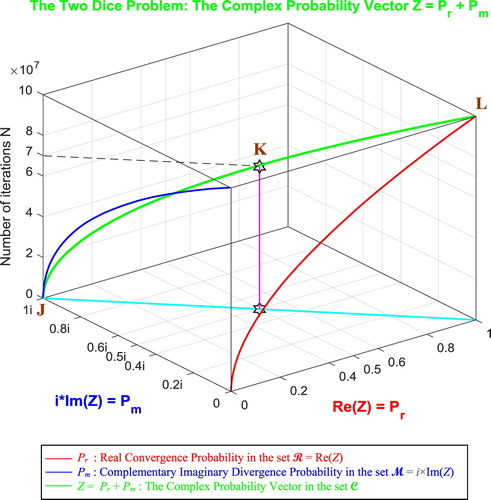
In the third cube (Figure 67), we can notice the simulation of the complex random vector Z(N) in $\mathcal{C}$ as a function of the real convergence probability P_r(N) = Re(Z) in $\mathcal{R}$ and of its complementary imaginary divergence probability P_m(N) = i × Im(Z) in $\mathcal{M}$, and this in terms of the iterations N for the two dice problem. The red curve represents P_r(N) in the plane P_m(N) = 0 and the blue curve represents P_m(N) in the plane P_r(N) = 0. The green curve represents the complex probability vector Z(N) = P_r(N) + P_m(N) = Re(Z) + i × Im(Z) in the plane P_r(N) = iP_m(N) + 1. The curve of Z(N) starts at the point J (P_r = 0, P_m = i, N = 0 iterations) and ends at the point L (P_r = 1, P_m = 0, N = N_C = 100,000,000 iterations). The line in cyan is P_r(0) = iP_m(0) + 1 and it is the projection of the Z(N) curve on the complex probability plane whose equation is N = 0 iterations. This projected line starts at the point J (P_r = 0, P_m = i, N = 0 iterations) and ends at the point (P_r = 1, P_m = 0, N = 0 iterations). Notice the importance of the point K corresponding to N = 70,000,000 iterations and when P_r = 0.5 and P_m = 0.5i. The three points J, K, L are the same as in Figure 64. At the end of all the simulations, it is crucial to mention here that all the previous examples (9.1.1 till 9.1.5 and 9.2.1 till 9.2.2) are illustrations of a linear convergence of the approximate result $R_A$ to the exact result $R_E$; therefore, the CPP parameters (P_r, MChf, DOK, P_m/i) meet at the middle of the simulation which is $\left(N_C/2,0.5\right)$ and the parameter Chf is minimal at $\left(N_C/2,-0.5\right)$ since $R_A$ converges linearly to $R_E$ (Figures 22, 27, 32, 37, 42, 48, 56). Actually, in these simulations, $N=N_C/2$corresponds to $R_A=R_E/2$. But in the last example and simulation (9.2.3: The two dice problem) we have the case of a nonlinear convergence of the approximate result $R_A$ to the exact result $R_E$ (Figures 60, 61, 62, 63); therefore, the CPP parameters (P_r, MChf, DOK, P_m/i) do not meet at the middle of the simulation which is $N_C/2$ but at $\left(N=70,000,000\text{ iterations},0.5\right)$ and the parameter Chf is minimal at $\left(N=70,000,000\text{ iterations},-0.5\right)$ since $R_A$ does not converge linearly to $R_E$ but it follows a nonlinear curve (Figure 64). Actually, in this simulation, $N=70,000,000\text{ iterations}$corresponds to $R_A=R_E/2$. These facts are the direct consequence of the solution of the stochastic problem in question and of the algorithm used in the simulation.

Figure 67. The Complex Probability Vector Z in terms of N for the two dice problem.

X. Conclusion and perspectives

In the present research work the novel extended Kolmogorov paradigm of eight axioms (EKA) was applied and bonded to the classical and stochastic Monte Carlo numerical methods. Hence, a tight link between Monte Carlo methods and the original paradigm was made. Therefore, the model of ‘Complex Probability’ was more elaborated beyond the scope of my previous twelve research works on this subject.

Additionally, as it was verified and shown in the novel model, when N = 0 (before the beginning of the random simulation) and when N = N_C (when Monte Carlo method converges to the exact result) therefore the degree of our knowledge (DOK) is one and the chaotic factor (Chf and MChf) is zero since the random effects and fluctuations have either not started or they have finished their task on the experiment. During the course of the stochastic experiment (0 < N < N_C) we have: 0.5 ≤ DOK < 1, −0.5 ≤ Chf < 0, and 0 < MChf ≤ 0.5. Notice that during this whole process we have always Pc² = DOK – Chf = DOK + MChf = 1 = Pc, that means that the simulation which looked to be stochastic and random in the set $\mathcal{R}$ is now certain and deterministic in the set $\mathcal{C}$ = $\mathcal{R}$ + $\mathcal{M}$, and this after the addition of the contributions of $\mathcal{M}$ to the phenomenon occurring in $\mathcal{R}$ and thus after subtracting and eliminating the chaotic factor from the degree of our knowledge. Moreover, the convergence and divergence probabilities of the stochastic Monte Carlo method corresponding to each iteration cycle N have been evaluated in the probability sets $\mathcal{R}$, $\mathcal{M}$, and $\mathcal{C}$ by $P_r$, $P_m$, and Pc respectively. Consequently, at each instance of N, the new Monte Carlo method and CPP parameters $R_E$,$R_A$, P_r, $P_m$, $P_m\text{/}i$, DOK, Chf, MChf, Pc, and Z are certainly and perfectly predicted in the complex probability set $\mathcal{C}$ with Pc maintained as equal to one constantly and permanently. In addition, using all these illustrated simulations and drawn graphs all over the whole research work, we can quantify and visualize both the certain knowledge (expressed by DOK and Pc) and the system chaos and random effects (expressed by Chf and MChf) of Monte Carlo methods. This is definitely very fascinating, fruitful, and wonderful and proves once again the advantages of extending the five probability axioms of Kolmogorov and thus the novelty and benefits of this original field in prognostic and applied mathematics that can be called verily: ‘The Complex Probability Paradigm’.

Furthermore, it is important to indicate here that one very well-known and essential probability distribution was considered in the present paper which is the discrete uniform probability distribution as well as a specific uniform random numbers generator, knowing that the novel CPP model can be applied to any uniform random numbers’ generator existent in literature. This will lead certainly to analogous conclusions and results and will show undoubtedly the success of my original theory.

Moreover, it is also significant to mention that it is possible to compare the current conclusions and results with the existing ones from both theoretical investigations and analysis and simulation researches and studies. This will be the task of subsequent research papers.

As a prospective and future work and challenges, it is planned to more elaborate the original created prognostic paradigm and to implement it to a varied set of nondeterministic systems like for other random experiments in classical probability theory and in stochastic processes. Furthermore, we will apply also CPP to the field of prognostic in engineering using the first order reliability method (FORM) as well as to the random walk problems which have enormous applications in physics, in economics, in chemistry, in applied and pure mathematics.

Disclosure statement

No potential conflict of interest was reported by the author.

ORCID

Abdo Abou Jaoude http://orcid.org/0000-0003-1851-4037

References

- Abou Jaoude, A. (2004, August 1). Ph.D. Thesis in Applied Mathematics: Numerical Methods and Algorithms for Applied Mathematicians. Bircham International University. Retrieved from http://www.bircham.edu
- Abou Jaoude, A. (2005, October). Ph.D. Thesis in Computer Science: Computer Simulation of Monté Carlo Methods and Random Phenomena. Bircham International University. Retrieved from http://www.bircham.edu
- Abou Jaoude, A. (2007, 27 April). Ph.D. Thesis in Applied Statistics and Probability: Analysis and Algorithms for the Statistical and Stochastic Paradigm. Bircham International University. Retrieved from http://www.bircham.edu
- Abou Jaoude, A. (2013a). The complex statistics paradigm and the law of large numbers. Journal of Mathematics and Statistics, Science Publications, 9(4), 289–304.
- Abou Jaoude, A. (2013b). The theory of complex probability and the first order reliability method. Journal of Mathematics and Statistics, Science Publications, 9(4), 310–324.
- Abou Jaoude, A. (2014). Complex probability theory and prognostic. Journal of Mathematics and Statistics, Science Publications, 10(1), 1–24.
- Abou Jaoude, A. (2015a). The complex probability paradigm and analytic linear prognostic for vehicle suspension systems. American Journal of Engineering and Applied Sciences, Science Publications, 8(1), 147–175.
- Abou Jaoude, A. (2015b). The paradigm of complex probability and the Brownian motion. Systems Science and Control Engineering, Taylor and Francis Publishers, 3(1), 478–503.
- Abou Jaoude, A. (2016a). The paradigm of complex probability and Chebyshev’s inequality. Systems Science and Control Engineering, Taylor and Francis Publishers, 4(1), 99–137.
- Abou Jaoude, A. (2016b). The paradigm of complex probability and analytic nonlinear prognostic for vehicle suspension systems. Systems Science and Control Engineering, Taylor and Francis Publishers, 4(1), 99–137.
- Abou Jaoude, A. (2017a). The paradigm of complex probability and analytic linear prognostic for unburied petrochemical pipelines. Systems Science and Control Engineering, Taylor and Francis Publishers, 5(1), 178–214.
- Abou Jaoude, A. (2017b). The paradigm of complex probability and Claude Shannon’s information theory. Systems Science and Control Engineering, Taylor and Francis Publishers, 5(1), 380–425.
- Abou Jaoude, A. (2017c). The paradigm of complex probability and analytic nonlinear prognostic for unburied petrochemical pipelines. Systems Science and Control Engineering, Taylor and Francis Publishers, 5(1), 495–534.
- Abou Jaoude, A. (2018). The paradigm of complex probability and Ludwig Boltzmann's entropy. Systems Science and Control Engineering, Taylor and Francis Publishers, 6(1), 108–149.
- Abou Jaoude, A. (2019a). The computer simulation of Monté Carlo methods and random phenomena. United Kingdom: Cambridge Scholars Publishing.
- Abou Jaoude, A. (2019b). The analysis of selected algorithms for the stochastic paradigm. United Kingdom: Cambridge Scholars Publishing.
- Abou Jaoude, A., El-Tawil, K., & Kadry, S. (2010). Prediction in complex dimension using Kolmogorov’s set of axioms. Journal of Mathematics and Statistics, Science Publications, 6(2), 116–124.
- Assaraf, R., Caffarel, M., & Khelif, A. (2000). Diffusion Monte Carlo methods with a fixed number of walkers. Physical Review E, 61(4), 4566–4575. doi:10.1103/physreve.61.4566. Bibcode:2000PhRvE..61.4566A. Archived from the original (PDF) on 2014-11-07.
- Barricelli, N. A. (1954). Esempi numerici di processi di evoluzione. Methodos, 1, 45–68.
- Barricelli, N. A. (1957). Symbiogenetic evolution processes realized by artificial methods. Methodos, 9, 143–182.
- Barrow, J. (1992). Pi in the sky. Oxford: Oxford University Press.
- Bell, E. T. (1992). The development of mathematics. New York: Dover Publications, Inc., United States of America.
- Benton, W. (1966a). Probability, encyclopedia Britannica (Vol. 18, pp. 570–574). Chicago: Encyclopedia Britannica Inc.
- Benton, W. (1966b). Mathematical probability, encyclopedia Britannica. (Vol. 18, pp. 574-579). Chicago: Encyclopedia Britannica Inc.
- Bidabad, B. (1992). Complex probability and markov stochastic processes. Proceeding first Iranian statistics conference, Tehran, Isfahan University of Technology.
- Bogdanov, I., & Bogdanov, G. (2009). Au commencement du Temps. Paris: Flammarion.
- Bogdanov, I., & Bogdanov, G. (2010). Le Visage de Dieu. Paris: Editions Grasset et Fasquelle.
- Bogdanov, I., & Bogdanov, G. (2012). La Pensée de Dieu. Paris: Editions Grasset et Fasquelle.
- Bogdanov, I., & Bogdanov, G. (2013). La Fin du Hasard. Paris: Editions Grasset et Fasquelle.
- Boursin, J.-L. (1986). Les Structures du Hasard. Paris: Editions du Seuil.
- Caffarel, M., Ceperley, D., & Kalos, M. (1993). Comment on Feynman–Kac path-integral calculation of the ground-state energies of atoms. Physical Review Letters, 71(13), 2159. Bibcode:1993PhRvL..71.2159C. doi:10.1103/physrevlett.71.2159. PMID 10054598.
- Carvalho, H., Del Moral, P., Monin, A., & Salut, G. (1997, July). Optimal non-linear filtering in GPS/INS integration. IEEE Transactions on Aerospace and Electronic Systems, 33(3), 835–850.
- Chan Man Fong, C. F., De Kee, D., & Kaloni, P. N. (1997). Advanced mathematics for applied and pure sciences. Amsterdam: Gordon and Breach Science Publishers, The Netherlands.
- Cox, D. R. (1955). A use of complex probabilities in the theory of stochastic processes. Mathematical Proceedings of the Cambridge Philosophical Society, 51, 313–319.
- Crisan, D., Del Moral, P., & Lyons, T. (1999). Discrete filtering using branching and interacting particle systems. Markov Processes and Related Fields, 5(3), 293–318.
- Crisan, D., Gaines, J., & Lyons, T. (1998). Convergence of a branching particle method to the solution of the Zakai. SIAM Journal on Applied Mathematics, 58(5), 1568–1590. doi: 10.1137/s0036139996307371
- Crisan, D., & Lyons, T. (1997). Nonlinear filtering and measure-valued processes. Probability Theory and Related Fields, 109(2), 217–244. doi: 10.1007/s004400050131
- Crisan, D., & Lyons, T. (1999). A particle approximation of the solution of the Kushner–stratonovitch equation. Probability Theory and Related Fields, 115(4), 549–578. doi: 10.1007/s004400050249
- Dacunha-Castelle, D. (1996). Chemins de l’Aléatoire. Paris: Flammarion.
- Dalmedico-Dahan, A., Chabert, J.-L., & Chemla, K. (1992). Chaos Et déterminisme. Paris: Edition du Seuil.
- Dalmedico-Dahan, A., & Peiffer, J. (1986). Une Histoire des Mathématiques. Paris: Edition du Seuil.
- Davies, P. (1993). The mind of god. London: Penguin Books.
- Del Moral, P. (1996). Nonlinear filtering: Interacting particle solution. Markov Processes and Related Fields, 2(4), 555–580.
- Del Moral, P. (1998). Measure valued processes and interacting particle systems. Application to nonlinear filtering problems. Annals of Applied Probability (Publications du Laboratoire de Statistique et Probabilités, 96–15 (1996) ed.), 8 (2), 438–495. CiteSeerX 10.1.1.55.5257. doi: 10.1214/aoap/1028903535
- Del Moral, P. (2003). Particle approximations of Lyapunov exponents connected to Schrödinger operators and Feynman–Kac semigroups. ESAIM Probability & Statistics, 7, 171–208. doi: 10.1051/ps:2003001
- Del Moral, P. (2004). Feynman–Kac formulae. Genealogical and interacting particle approximations. Berlin: Springer. pp. 575. Series: Probability and Applications.
- Del Moral, P., & Guionnet, A. (1999). On the stability of measure valued processes with applications to filtering. Comptes Rendus de L'Académie des Sciences - Series I - Mathematics, 329(1), 429–434.
- Del Moral, P., & Guionnet, A. (2001). On the stability of interacting processes with applications to filtering and genetic algorithms. Annales de L'Institut Henri Poincaré, 37(2), 155–194. Bibcode:2001AnIHP..37..155D. doi: 10.1016/s0246-0203(00)01064-5
- Del Moral, P., & Miclo, L. (2000a). Branching and interacting particle systems approximations of Feynman–Kac formulae with applications to non-linear filtering. In Séminaire de Probabilités, XXXIV. Lecture Notes in mathematics. 1729 (pp. 1–145). Berlin: Springer. doi:10.1007/BFb0103798. ISBN 978-3-540-67314-9. MR 1768060.
- Del Moral, P., & Miclo, L. (2000b). A Moran particle system approximation of Feynman–Kac formulae. Stochastic Processes and Their Applications, 86(2), 193–216. doi: 10.1016/S0304-4149(99)00094-0
- Del Moral, P., Noyer, J.-C., Rigal, G., & Salut, G. (1992c, December). Particle filters in radar signal processing: detection, estimation and air targets recognition. LAAS-CNRS, Toulouse, Research report no. 92495.
- Del Moral, P., Rigal, G., & Salut, G. (1991, April). Estimation and nonlinear optimal control: A unified framework for particle solutions. LAAS-CNRS, Toulouse, Research Report no. 91137, DRET-DIGILOG- LAAS/CNRS contract.
- Del Moral, P., Rigal, G., & Salut, G. (1991, September). Nonlinear and non-Gaussian particle filters applied to inertial platform repositioning. LAAS-CNRS, Toulouse, Research Report no. 92207, STCAN/DIGILOG-LAAS/CNRS Convention STCAN no. A.91.77.013, (94pp.).
- Del Moral, P., Rigal, G., & Salut, G. (1992, January). Estimation and nonlinear optimal control: Particle resolution in filtering and estimation. Experimental results. Convention DRET no. 89.34.553.00.470.75.01, Research report no.2 (54pp.).
- Del Moral, P., Rigal, G., & Salut, G. (1992, October). Estimation and nonlinear optimal control: Particle resolution in filtering and estimation. Theoretical results Convention DRET no. 89.34.553.00.470.75.01, Research report no.3 (123pp.).
- Del Moral, P., Rigal, G., & Salut, G. (1993, January). Estimation and nonlinear optimal control: Particle resolution in filtering and estimation. Studies on: Filtering, optimal control, and maximum likelihood estimation. Convention DRET no. 89.34.553.00.470.75.01. Research report no.4 (210pp.).
- Eckhardt, R. (1987). Stan Ulam, John von Neumann, and the Monte Carlo method. Los Alamos Science, 1(15), 131–137.
- Ekeland, I. (1991). Au Hasard. La chance, la science et Le Monde. Paris: Editions du Seuil.
- Fagin, R., Halpern, J., & Megiddo, N. (1990). A logic for reasoning about probabilities. Information and Computation, 87, 78–128.
- Feller, W. (1968). An introduction to probability theory and its applications (3rd ed.). New York: Wiley.
- Fermi, E., & Richtmyer, R. D. (1948). Note on census-taking in Monte Carlo calculations. LAM, 805(A), 1–33, Declassified report Los Alamos Archive.
- Freund, J. E. (1973). Introduction to probability. New York: Dover Publications.
- Gentle, J. (2003). Random number generation and Monté Carlo methods (2nd ed). Sydney: Springer.
- Gillies, D. (2000). Philosophical theories of probability. London: Routledge. ISBN 978-0415182768.
- Gleick, J. (1997). Chaos, making a new science. New York: Penguin Books.
- Gordon, N. J., Salmond, D. J., & Smith, A. F. M. (1993, April). Novel approach to nonlinear/non-Gaussian Bayesian state estimation. IEE Proceedings F Radar and Signal Processing, 140(2), 107–113. doi:10.1049/ip-f-2.1993.0015. ISSN 0956-375X.
- Guillen, M. (1995). Initiation Aux Mathématiques. Paris: Albin Michel.
- Gullberg, J. (1997). Mathematics from the birth of numbers. New York: W.W. Norton & Company.
- Hawking, S. (2002). On the shoulders of giants. London: Running Press.
- Hawking, S. (2005). God created the integers. London: Penguin Books.
- Hawking, S. (2011). The dreams that stuff is made of. London: Running Press.
- Herman, K., & Theodore, H. E. (1951). Estimation of particle transmission by random sampling. Natl. Bur. Stand. Appl. Math. Ser, 12, 27–30.
- Hetherington, J. H. (1984). Observations on the statistical iteration of matrices. Physical Review A, 30(2713), 2713–2719. Bibcode:1984PhRvA..30.2713H. doi: 10.1103/PhysRevA.30.2713
- Kitagawa, G. (1996). Monte Carlo filter and smoother for non-Gaussian nonlinear state space models. Journal of Computational and Graphical Statistics, 5(1), 1–25. doi:10.2307/1390750. JSTOR 1390750.
- Mazhdrakov, M., Benov, D., & Valkanov, N. (2018). The Monte Carlo method. Engineering applications. Cambridge, MA: ACMO Academic Press. pp. 250. ISBN 978-619-90684-3-4.
- McKean, H. P. (1966). A class of Markov processes associated with nonlinear parabolic equations. Proceedings of the National Academy of Sciences of the United States of America, 56(6), 1907–1911. doi:10.1073/pnas.56.6.1907. Bibcode:1966PNAS … 56.1907M. PMC 220210. PMID 16591437.
- McKean, H. P. (1967). Propagation of chaos for a class of nonlinear parabolic equations. Lecture Series in Differential Equations, Catholic University, pp. 41–57. Arlington, VA: Air Force Office Sci. Res.
- Metropolis, N. (1987). The beginning of the Monte Carlo method. Los Alamos Science, (1987 Special Issue dedicated to Stanislaw Ulam), 1, 125–130.
- Montgomery, D. C., & Runger, G. C. (2003). Applied statistics and probability for Engineers (3rd ed). New York: John Wiley & Sons, Inc.
- Ognjanović, Z., Marković, Z., Rašković, M., Doder, D., & Perović, A. (2012). A probabilistic temporal logic that can model reasoning about evidence. Annals of Mathematics and Artificial Intelligence, 65, 1–24.
- Peragine, M. (2013). The universal mind: The evolution of machine intelligence and human psychology. San Diego, CA: Xiphias Press.
- Pickover, C. (2008). Archimedes to hawking. Oxford: Oxford University Press.
- Rosenbluth, M. N., & Rosenbluth, A. W. (1955). Monte-Carlo calculations of the average extension of macromolecular chains. The Journal of Chemical Physics, 23(2), 356–359. Bibcode:1955JChPh..23..356R. doi: 10.1063/1.1741967
- Science Et Vie. (1999). Le Mystère des Mathématiques. Numéro, 984.
- Srinivasan, S. K., & Mehata, K. M. (1988). Stochastic processes (2nd ed.). New Delhi: McGraw-Hill.
- Stepić, A. I., & Ognjanović, Z. (2014). Complex valued probability logics. Publications De L’institut Mathématique, Nouvelle Série, Tome, 95(109), 73–86. doi: 10.2298/PIM1409073I
- Stewart, I. (1996). From here to infinity (2nd ed.). Oxford: Oxford University Press.
- Stewart, I. (2002). Does god play dice? (2nd ed.). Oxford: Blackwell Publishing.
- Stewart, I. (2012). In pursuit of the unknown. New York: Basic Books.
- Turing, A. M. (1950). Computing machinery and intelligence. Mind; A Quarterly Review of Psychology and Philosophy, LIX(238), 433–460. doi: 10.1093/mind/LIX.236.433
- Van Kampen, N. G. (2006). Stochastic processes in physics and chemistry. Revised and enlarged edition. Sydney: Elsevier.
- Walpole, R., Myers, R., Myers, S., & Ye, K. (2002). Probability and statistics for Engineers and Scientists (7th ed). New Jersey: Prentice Hall.
- Wei, Y., Park, J. H., Qiu, J., Wu, L., & Jung, H. Y. (2017, July). Sliding mode control for Semi-Markovian jump systems Via output feedback. Automatica, 81, 133–141.
- Wei, Y., Qiu, J., Karimi, H. R., & Ji, W. (2017, October). A novel Memory filtering Design for Semi-Markovian Jump time-Delay systems. IEEE Transactions on systems, Man, and Cybernetics: Systems, (pp. 2229–2241).
- Weingarten, D. (2002). Complex probabilities on RN as real probabilities on CN and an application to path integrals. Physical Review Letters, 89, 335. doi: 10.1103/PhysRevLett.89.240201
- Wikipedia, the free encyclopedia, Monte Carlo Method. Retrieved from https://en.wikipedia.org/
- Wikipedia, the free encyclopedia. Probability. Retrieved from https://en.wikipedia.org/
- Wikipedia, the free encyclopedia, Probability Axioms. Retrieved from https://en.wikipedia.org/
- Wikipedia, the free encyclopedia, Probability Density Function. Retrieved from https://en.wikipedia.org/
- Wikipedia, the free encyclopedia, Probability Distribution. Retrieved from https://en.wikipedia.org/
- Wikipedia, the free encyclopedia. Probability Interpretations. Retrieved from https://en.wikipedia.org/
- Wikipedia, the free encyclopedia, Probability Measure. Retrieved from https://en.wikipedia.org/
- Wikipedia, the free encyclopedia, Probability Theory. Retrieved from https://en.wikipedia.org/
- Wikipedia, the free encyclopedia, Stochastic Process. Retrieved from https://en.wikipedia.org/
- Wikipedia, the free encyclopedia, Probability Space. Retrieved from https://en.wikipedia.org/
- Youssef, S. (1994). Quantum mechanics as complex probability theory. Modern Physics Letters A, 9, 2571–2586.