An adaptive approach for vehicle suspension system control in presence of uncertainty and unknown actuator time delay

Abstract

This paper presents an adaptive approach for controlling the nonlinear vehicle suspension system in the presence of unknown delay and limited disturbance. All three factors present in the quarter vehicle suspension model including uncertainty, disturbance and input delay are limited but unknown. This paper dealings a nonlinear model to describe more accurately the behaviour of the suspension and the controller design. To prove stability in the Lyapunov concept, the proposed control method is a combination of backstepping and adaptive approaches. The results of the simulation confirm better active suspension performance regardless of the unknown time delay, disturbances and uncertainty in the nonlinear model.

KEYWORDS:

• Quarter vehicle suspension system
• unknown actuator time delay
• adaptive approach
• backstepping approach
• uncertainty
• disturbances

1. Introduction

Vehicle suspensions play an important role in modern vehicles, providing inconsistent vehicle suspension performances, such as ride comfort, road holding, and suspension deflection. These features of the suspension system keep the contact between the vehicle's tire and the road surface to ensure the stability of the vehicles and provide a comfortable ride by isolating passengers from the vibration and shock of the road (García-Rodríguez et al., 2009; Hrovat, 1997; Montazeri-Gh & Soleymani, 2010). Generally, due to the incompatibility of the mentioned performance characteristics, the achievement of proper performance is followed by a compromise obtained from a controller (Gao et al., 2010; Sun et al., 2011, 2012).

Suspensions can be classified into three categories: passive suspension, semi-active suspension and active suspension (Amirifar & Sadati, 2006; Cao et al., 2008; Poussot-Vassal et al., 2008), among which the active suspension is the most effective way to improve suspension performance and many studies have been done in this area (Cao et al., 2010; Gao et al., 2006; Yamashita et al., 1994). To compromise the conflicting tasks of suspension system, active suspension control approaches have been adopted based on various control techniques such as the H∞ method (Chen & Guo, 2005; Du & Zhang, 2007) along with the Lyapunov-Krasovkii functional method (Chen, 2007; Goldhirsch et al., 1987) and the linear matrix inequality (LMI) approach (Boyd et al., 1994).

There are three main topics in the active control of the suspension system that has received little attention, or to put it simply, these three concerns are not considered simultaneously in active suspension control. They are:

1. The existence of a delay in the hydrodynamic actuator.

2. Nonlinear behaviour of the suspension system.

3. Disturbances in the system and uncertainties in the model.

We now describe each of these cases and their effects. Because of the superiority of hydraulic actuators to electromagnetic, these actuators are used in the vehicle suspension system. When tracking a desired force, particularly there is a time delay in this actuator that ignoring it would undermine the system stability and control performance.

It is obvious that the suspension actuator with time delay is one of the key factors in the next generation of active suspension control systems (Jalili & Esmailzadeh, 2001; Lei & Tang, 2008; Vahidi & Eskandarian, 2001).

Jalili and Esmailzadeh (2001) fully describe the dynamics of the actuator used in the suspension system and shows that the delay in the actuator is influenced by various parameters such as vehicle speed and movement, sprung and unsprung mass levels as well as irregular road conditions and so the delay is not constant. The variability of the delay has also been shown in other references (Choi et al., 2016; Du & Zhang, 2007).

Thus, the time delay of the actuator should be taken into account in the control design of active suspension systems for the improvement of performance. Recently, attempts to address the effect of actuator time delays have been made in Du et al., (2008), Du and Zhang (2007), Du and Zhang (2008), Jalili and Esmailzadeh (2001), Vahidi and Eskandarian (2001), Wang and Wilson (2001). However, only a few research studies have produced meaningful results. For the expansion of allowable time delay, analytical techniques and synthesis methods that reduce conservatism need to be developed in active suspension systems.

Another important issue regarding the suspension system is its nonlinear behaviour. Due to the material properties and also due to nonlinear compression and rebound, the existence of bump stops, tire lifts in some suspension systems and also due to the nonlinearity of the strut bushing in the damper, the suspension dynamics are quite nonlinear.

Because of the complex mathematical relationships in an actual suspension system, most researchers approximate it to a linear model. When the system is subject to major dash due to rough roads, the states exhibit large deviations from the equilibrium point and rotational inertias can become significant contributors to the system behaviour, making a more comprehensive nonlinear model worthy of investigation. Therefore, to study the suspension behaviour effectively, it is necessary to consider its nonlinear model and apply it for designing the controller. So far, various nonlinear mathematical models have been developed (Haris & Aboud, 2016; Hassanzadeh et al., 2010; Nagarkar et al., 2016). The models are more or less complex depending on the requirement sets and intended use.

Another problem to be noted is uncertainty and disturbance of the model. In practice, disturbance occurs in many engineering tasks that lead to undesirable behaviour and the suspension system is no exception. Practical considerations of the realization of active suspensions in real-world applications should also include uncertainties.

Depending on the weight of the load and the number of passengers, the weight of the sprung and unsprung masses changes in the active suspension system and if the changes are not considered in the controller design process, the performance of suspension system will be affected. Given the importance of the uncertainties in suspension system operation, this has been well followed in some references (Du et al., 2008; Gao et al., 2006; Gao et al., 2010; Li et al., 2012).

Despite of many studies on suspension control, none of the control methods have been able to cover these effects simultaneously to date, while these effects on suspension dynamics are certain. How to design a controller and achieve the performances will be a challenge when the non-linear delayed suspension is associated with uncertainty and disturbance. Therefore, this paper focuses on the problem of controlling the nonlinear uncertain suspension system with disturbance and unknown input delay, which has not been addressed to date. Therefore, this paper proposes a new adaptive method for controlling the nonlinear suspension model that considers the above effects. The delay imposed by the actuator is considered to be variable and, although this delay is bounded, it is assumed that we have no knowledge on the upper bound of the delay. In the nonlinear model of the system, it is assumed that boundary disturbance exists with the unknown upper bound, and in this paper, the uncertainty upper bound is also considered unknown. Finally, with the proposed control method in the presence of unknown delay in the input, disturbance and uncertainty with an unknown upper bound, as well as considering the nonlinear model, the stability of the system in Lyapunov concept is guaranteed. Now this article is organized as follows: In the second part, a non-linear model of the suspension system with delayed actuator is presented. In the third section, the proposed control method is presented. In the fourth and fifth sections, the simulation results and conclusions are presented, respectively.

2. Suspension model with delayed actuator

Figure 1 shows the 1/4 vehicle model considered in this paper for designing of the active suspension control law. This model is deduced from very important features in detailed models of papers (Barethiye et al., 2017; Sun et al., 2014). The equations of motion for sprung mass and unsprung mass are: (1) $\begin{array}{rl}& m_s{\ddot{z}}_s+F_d+F_s=u\left(t-\tau \right)+F_l\\ & m_u{\ddot{z}}_u-F_d-F_s+F_t+F_b=-u\left(t-\tau \right)\end{array}$(1) where $\begin{array}{rl}{F}_d& =\left\{\begin{array}{c}{b}_e\left({\dot{z}}_s-{\dot{z}}_u\right){\dot{z}}_s-{\dot{z}}_u>0\\ b_c\left({\dot{z}}_s-{\dot{z}}_u\right){\dot{z}}_s-{\dot{z}}_u\le 0\end{array}\right.\end{array}$ $\begin{array}{rl}{F}_t& =k_f\left(z_u-z_r\right)\end{array}$ $\begin{array}{rl}{F}_b& =b_f\left({\dot{z}}_u-{\dot{z}}_r\right)\end{array}$ $\begin{array}{rl}{F}_s& =k_{s1}\left(z_s-z_u\right)+k_{n1}(z_s-z_u{)}^3\end{array}$

Figure 1. A quarter vehicle model with active suspension.

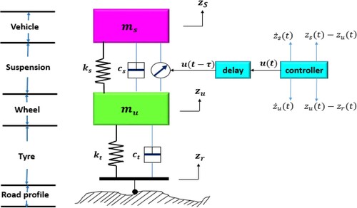
where in the above equations $z_s\left(t\right)$and $z_u\left(t\right)$ are respectively the displacement of the sprung mass and the unsprung mass; $m_s$ is the sprung mass, which represents the vehicle chassis; $m_u$ is unsprung mass, which represents the set of wheels; $F_l$ represents the friction force of the suspension components, and $F_s$ represents the forces generated by nonlinear strengthening springs, piece-linear damper, and tire. $k_{s1}$ and $k_{n1}$ are the stiffness coefficient of the linear terms and the stiffness coefficient of the cubic terms, respectively; $b_e$ is the damping coefficient for the extension movement and $b_c$ is the damping coefficient for the compression movement; $k_f,b_f$ are the stiffness and damping coefficients of the tires.

By defining state variables as follows: (2) $\begin{array}{rl}{x}_1\left(t\right)& =z_s\left(t\right)\\ x_2\left(t\right)& ={\dot{z}}_s\left(t\right)\\ x_3\left(t\right)& =z_u\left(t\right)\\ x_4\left(t\right)& ={\dot{z}}_u\left(t\right)\end{array}$(2) We get this set of equations: (3) $\begin{array}{rl}& {\dot{x}}_1=x_2\\ & m_s{\dot{x}}_2=\psi \left(x,t\right)+u\left(t-\tau \right)+F_l\\ & {\dot{x}}_3=x_4\\ & m_u{\dot{x}}_4=-\psi \left(x,t\right)-F_t-F_b-u\left(t-\tau \right)\end{array}$(3) where $m_s\in {\mathrm{\Omega }}_m=\left\{m_s:m_{smin}\le m_s\le m_{smax}\right\}$ $|\psi \left(x,t\right)=-F_d-F_s|\le h$ $|F_l|\le d,$$h$ and $d$ are positive constants.

3. Suspension control

By rewriting the suspension as follows in the state space (4) $\begin{array}{rl}& {\dot{x}}_1=x_2\\ & m_s{\dot{x}}_2=\psi \left(x,t\right)+u_h+f_L\\ & {\dot{x}}_3=x_4\\ & m_u{\dot{x}}_4=-\psi \left(x,t\right)-f_t-f_b-u_h\end{array}$(4) where $u_h$ is delayed input and $y$ is system output as follows: (5) $\begin{array}{rl}& y=x_1\\ & u_h=u\left(t-h\left(t\right)\right)\end{array}$(5) We define the error variables as follows: (6) $\begin{array}{rl}{z}_1& =y-y_d\\ z_2& =x_2-{\alpha }_1+\frac{1}{m_s}{z}_u\\ z_3& =x_3\\ z_4& =x_4-{\alpha }_2+\frac{1}{m_u}{z}_u\\ z_u& ={\int }_{t-h\left(t\right)}^{t}u\left(v\right)dv\end{array}$(6) where ${\alpha }_1$ and ${\alpha }_2$ are virtual control vectors and are defined as follows. (7) $\begin{array}{rl}{\alpha }_1& =-k_1{z}_1+{\dot{y}}_d+\frac{1}{m_u}{\hat{z}}_u\\ {\alpha }_2& =-k_3{z}_3-\frac{1}{m_u}{\hat{z}}_u\end{array}$(7) Now, by choosing the Lyapunov function as follows: (8) $\begin{array}{rl}V& =\frac{1}{2}{z}_1^2+\frac{1}{2}{z}_2^2+\frac{1}{2}{z}_3^2+\frac{1}{2}{z}_4^2+\frac{1}{2{\lambda }_1{m}_s}{\tilde{w}}_1^2\\ & +\frac{1}{2{\lambda }_1{m}_u}{\tilde{w}}_2^2+\frac{1}{2{\lambda }_3}{\tilde{z}}_u^2\end{array}$(8) where ${\tilde{w}}_1=w_1-{\hat{w}}_1,{\tilde{w}}_2=w_2-{\hat{w}}_2,{\tilde{z}}_u=z_u-{\hat{z}}_u$By deriving the Lyapunov function, we have: (9) $\begin{array}{rl}\dot{V}& =-k_1{z}_1^2+z_1{z}_2-\frac{1}{m_s}{z}_1{\tilde{z}}_u-k_3{z}_3^2+z_3{z}_4+\frac{1}{m_u}{z}_3{\tilde{z}}_u\\ & +z_2\left(\frac{1}{m_s}\right(\psi \left(x,t\right)+u_h+f_L)-{\dot{\alpha }}_1+\frac{1}{m_s}{\dot{z}}_u\\ & +z_4\left(\frac{-1}{m_u}\left(\psi \left(x,t\right)+f_t+f_b+u_h\right)-{\dot{\alpha }}_2-\frac{1}{m_u}{\dot{z}}_u\right)\\ & -\frac{1}{{\lambda }_1{m}_s}{\tilde{w}}_1{\dot{\hat{w}}}_1-\frac{1}{{\lambda }_2{m}_u}{\tilde{w}}_1{\dot{\hat{w}}}_2-\frac{1}{{\lambda }_3}{\tilde{z}}_u{\dot{\hat{z}}}_u\end{array}$(9) With the adaptive law for ${\hat{z}}_u$ as follows (10) ${\dot{\hat{z}}}_u={\lambda }_3\left(\frac{1}{m_u}{z}_3-\frac{1}{m_s}{z}_1\right)$(10) By replacing Equation (10) in Equation (9), it is obtained (11) $\begin{array}{rl}\dot{V}& =-k_1{z}_1^2-k_3{z}_3^2+z_1{z}_2+z_3{z}_4\\ & +{\tilde{z}}_u\left(\left(\frac{1}{m_u}{z}_3-\frac{1}{m_s}{z}_1\right)-\frac{1}{{\lambda }_3}{\dot{\hat{z}}}_u\right)\\ & +z_2\left(\frac{1}{m_s}\left(\psi \left(x,t\right)+f_L+u+\dot{h}{u}_h\right)-{\dot{\alpha }}_1\right)\\ & +z_4\left(\frac{-1}{m_u}\left(\psi \left(x,t\right)+f_t+f_b+u+\dot{h}{u}_h\right)-{\dot{\alpha }}_2\right)\\ & -\frac{1}{{\lambda }_1{m}_s}{\tilde{w}}_1{\dot{\hat{w}}}_1-\frac{1}{{\lambda }_2{m}_u}{\tilde{w}}_2{\dot{\hat{w}}}_2\end{array}$(11) By defining the control signal $u$, and $w_1$ and $w_2$ as terms containing uncertainty, input delay and nonlinear parts, we have (12) $\begin{array}{rl}u\left(t\right)& =-\psi \left(x,t\right)+u_1\left(t\right)+u_2\left(t\right)\\ w_1& =u_2+f_L+\dot{h}{u}_h\\ w_2& =u_1+f_t+f_b+\dot{h}{u}_h\end{array}$(12) By replacing Equation 12 in Equation 11, it is obtained (13) $\begin{array}{rl}\dot{V}& =-k_1{z}_1^2-k_3{z}_3^2+z_1{z}_2+z_3{z}_4\\ & +z_2\left(\frac{1}{m_s}\left(w_1+u_1\right)-{\dot{\alpha }}_1\right)\\ & +z_4\left(\frac{-1}{m_u}\left(w_2+u_2\right)-{\dot{\alpha }}_2\right)\\ & -\frac{1}{{\lambda }_1{m}_s}{\tilde{w}}_1{\dot{\hat{w}}}_1-\frac{1}{{\lambda }_2{m}_u}{\tilde{w}}_2{\dot{\hat{w}}}_2\end{array}$(13) To stabilize the system based on Lyapunov function, $u_1$ and $u_2$ control signals are selected as follows: (14) $\begin{array}{rl}{u}_1\left(t\right)& =-{\hat{w}}_1+m_s\left({\dot{\alpha }}_1-z_1-k_2{z}_2\right)\\ u_2\left(t\right)& =-{\hat{w}}_2+m_u\left({\dot{\alpha }}_2-z_3-k_4{z}_4\right)\end{array}$(14) By replacing the control signals $u_1$ and $u_2$ in Equation 13, the derivative of the Lyapunov function is simplified as follows: (15) $\begin{array}{rl}\dot{V}& =-k_1{z}_1^2-k_2{z}_2^2-k_3{z}_3^2-k_4{z}_4^2\\ & +\frac{1}{m_s}\left({\tilde{w}}_1\left(z_2-\frac{1}{{\lambda }_1}{\dot{\hat{w}}}_1\right)\right)\\ & -\frac{1}{m_u}\left({\tilde{w}}_2\left(z_4-\frac{1}{{\lambda }_2}{\dot{\hat{w}}}_2\right)\right)\end{array}$(15) By selecting the adaptive laws for ${\hat{w}}_1$ and ${\hat{w}}_2$ as follows (16) $\begin{array}{rl}{\dot{\hat{w}}}_1& ={\lambda }_1{z}_2\\ {\dot{\hat{w}}}_2& =-{\lambda }_2{z}_4\end{array}$(16) Finally we will get to the following equation. (17) $\dot{V}=-k_1{z}_1^2-k_2{z}_2^2-k_3{z}_3^2-k_4{z}_4^2\le 0$(17) Which indicates the stability of the suspension system under the proposed controller.

4. Simulation results

The results of the implementation of the proposed control method on the active suspension system are presented here. The values of the suspension parameters are the same as the reference (Sun et al., 2014). Also the values of the parameters used in the controller are as follows: $k_1={10}^3,k_2=1,k_3=1,k_4=1$ ${\lambda }_1={10}^{-3},{\lambda }_1={10}^{-3}$To illustrate the capability of the proposed method, four simulation scenarios are considered, and we will now describe each of these scenarios.

4.1. First scenario

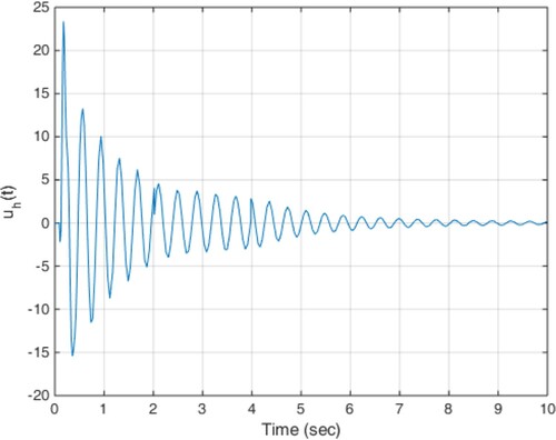
In this case, a bump disturbance in the following form is considered as road disturbance: (18) $z_r\left(t\right)=\left\{\begin{array}{ll}\frac{H}{2}\left(1-\cos \left(\frac{2\pi V}{L}t\right)\right),& if0\le t\le \frac{L}{V}\\ 0,& ift\ge \frac{L}{V}\end{array}\right.$(18) The constant delay of 10 milliseconds is considered as the actuator delay. The simulation results are given in Figures 2–6. As can be seen from Figures 2–5, the proposed method is able to meet the performance specifications required for the active suspension system and specifically targeted ride comfort is well followed due to Figures 2 and 3. In Figure 6, the control signal is shown.

Figure 2. Displacement response of the sprung mass in scenario 1.

Figure 3. Acceleration response of the sprung mass in scenario 1.

Figure 4. Displacement response of the unsprung mass in scenario 1.

Figure 5. Acceleration response of the unsprung mass in scenario 1.

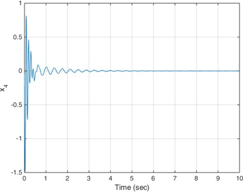
Figure 6. Trajectory of control effort of the proposed method in scenario 1.

4.2. Second scenario

In this case, the following disturbance intended as a rough road surface and actuator time delay is fixed to 10 milliseconds. (19) $\begin{array}{rl}{z}_r\left(t\right)& =0.0254\sin \left(2\pi t\right)+0.005\sin \left(10.5\pi t\right)\\ & +0.001\sin \left(21.5\pi t\right)\left(m\right)\end{array}$(19) The results of the implementation of the proposed method are presented in Figures 7–11. Due to the states shown, such as low displacement and low acceleration of the car body, ride comfort and low deflection of the suspension are guaranteed.

Figure 7. Displacement response of the sprung mass in scenario 2.

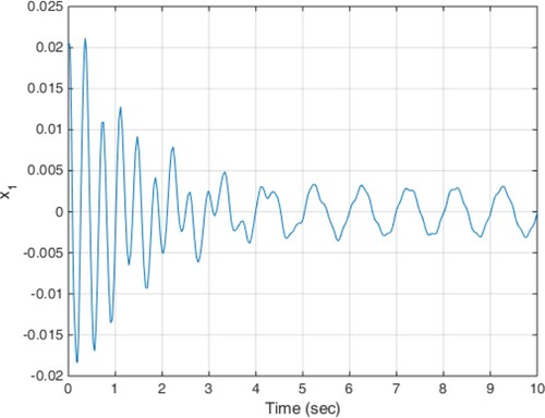
Figure 8. Acceleration response of the sprung mass in scenario 2.

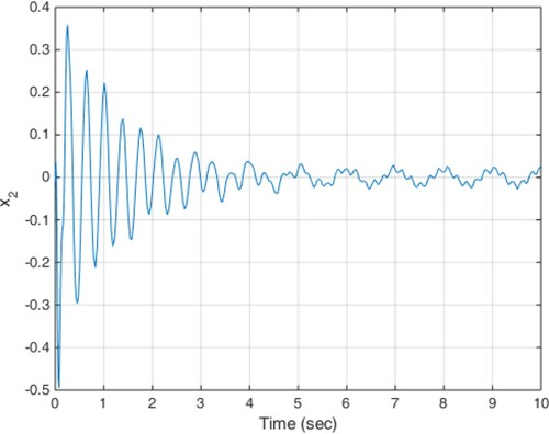
Figure 9. Displacement response of the unsprung mass in scenario 2.

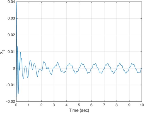
Figure 10. Acceleration response of the unsprung mass in scenario 2.

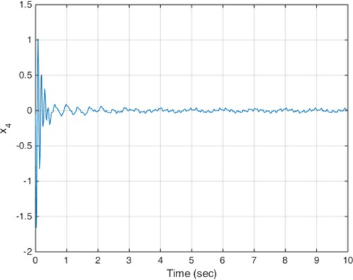
Figure 11. Trajectory of control effort of the proposed method in scenario 2.

4.3. The third scenario

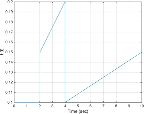
This scenario is similar to the first case, and disturbance at (18) is considered as roadside disturbance, but the delay of the actuator is time-varying and its profile is shown in Figure 12.

Figure 12. Actuator time-varying delay profile used in the simulation.

The results of the implementation of the proposed control method are shown in Figures 13–17. Achieving stability and performance characteristics of the suspension system despite of the adverse impact of time-varying delay is one of the results obtained in this scenario.

Figure 13. Displacement response of the sprung mass in scenario 3.

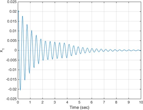
Figure 14. Acceleration response of the sprung mass in scenario 3.

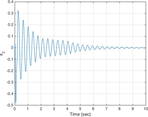
Figure 15. Displacement response of the unsprung mass in scenario 3.

Figure 16. Acceleration response of the unsprung mass in scenario 3.

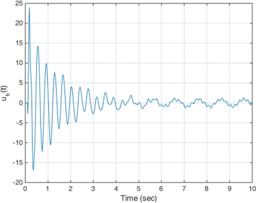
Figure 17. Trajectory of control effort of the proposed method in scenario 3.

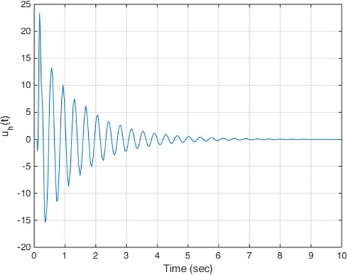
4.4. The fourth scenario

In this case, the input disturbance from the road is in the form of Equation (19) and the actuator time-varying delay profile is shown in Figure 12. The results of the simulation are also shown in Figures 18–22. As it is clear from the figures, such as previous scenarios the proposed controller is able to provide the ride comfort and low deflection of the suspension system in a short time despite of the actuator variable time delay.

Figure 18. Displacement response of the sprung mass in scenario 4.

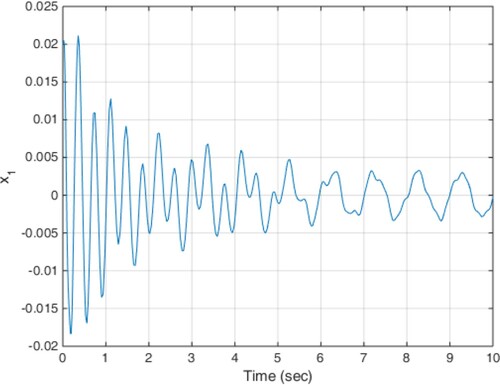
Figure 19. Acceleration response of the sprung mass in scenario 4.

Figure 20. Displacement response of the unsprung mass in scenario 4.

Figure 21. Acceleration response of the unsprung mass in scenario 4.

Figure 22. Trajectory of control effort of the proposed method in scenario 4.

According to the simulation results, the proposed method is able to compensate any time-varying delay at the input and at the same time, uncertainty and disturbance effects are well covered and the robust stability of the system is ensured by minimizing the impact of road disturbances on system performance. The smooth behaviour of the obtained control signals is another desirable characteristic of the proposed method.

5. Conclusion

In this paper, suspension control in the presence of time-varying delay is studied. Because of the benefits of the nonlinear model in describing the dynamics of the system more accurately, this model has been used in controller design. The presence of disturbance and uncertainty in the proposed control method is also considered. Using Lyapunov's theory, closed-loop suspension stability is guaranteed under the proposed adaptive controller, while performance is satisfied and the upper bound of disturbance and uncertainty as well as delay are assumed to be unknown. In different simulation scenarios, the controller performance was verified. For future work, the proposed method can be extended to a wider class of nonlinear systems plus considering constraints.

Disclosure statement

No potential conflict of interest was reported by the author(s).

References

- Amirifar, R., & Sadati, N. (2006). Low-order H∞ controller design for an active suspension system via LMIS. IEEE Transactions on Industrial Electronics, 53(2), 554–560. https://doi.org/https://doi.org/10.1109/TIE.2006.870672
- Barethiye, V. M., Pohit, G., & Mitra, A. (2017). Analysis of a quarter car suspension system based on nonlinear shock absorber damping models. International Journal of Automotive and Mechanical Engineering, 14(3), 4401–4418. https://doi.org/https://doi.org/10.15282/ijame.14.3.2017.2.0349
- Boyd, S., El Ghaoui, L., Feron, E., & Balakrishnan, V. (1994). Linear matrix inequalities in system and control theory. SIAM.
- Cao, J., Li, P., & Liu, H. (2010). An interval fuzzy controller for vehicle active suspension systems. IEEE Transactions on Intelligent Transportation Systems, 11(4), 885–895. https://doi.org/https://doi.org/10.1109/TITS.2010.2053358
- Cao, J., Liu, H., Li, P., & Brown, D. (2008). State of the art in vehicle active suspension adaptive control systems based on intelligent methodologies. IEEE Transactions on Intelligent Transportation Systems, 9(3), 392–405. https://doi.org/https://doi.org/10.1109/TITS.2008.928244
- Chen, H. (2007). A feasible moving horizon H∞ control scheme for constrained uncertain linear systems. IEEE Transactions on Automatic Control, 52(2), 343–348. https://doi.org/https://doi.org/10.1109/TAC.2006.890373
- Chen, H., & Guo, K. (2005). Constrained H∞ control of active suspensions: An LMI approach. IEEE Transactions on Control Systems Technology, 13(3), 412–421. https://doi.org/https://doi.org/10.1109/TCST.2004.841661
- Choi, H. D., Ahn, C. K., Lim, M. T., & Song, M. K. (2016). Dynamic output-feedback H∞ control for active half-vehicle suspension systems with time-varying input delay. International Journal of Control, Automation and Systems, 14(1), 59–68. https://doi.org/https://doi.org/10.1007/s12555-015-2005-8
- Du, H., & Zhang, N. (2007). H∞ control of active vehicle suspensions with actuator time delay. Journal of Sound and Vibration, 301(1/2), 236–252. https://doi.org/https://doi.org/10.1016/j.jsv.2006.09.022
- Du, H., & Zhang, N. (2008). Constrained H! control of active suspension for a half-car model with a time delay in control. Proceedings of the Institution of Techanical Engineers, Part D: Journal of Automobile Engineering, 222(5), 665–684. https://doi.org/https://doi.org/10.1243/09544070JAUTO299
- Du, H., Zhang, N., & Lam, J. (2008). Parameter-dependent input-delayed control of uncertain vehicle suspensions. Journal of Sound and Vibration, 317(3–5), 537–556. https://doi.org/https://doi.org/10.1016/j.jsv.2008.03.066
- Gao, H., Lam, J., & Wang, C. (2006). Multi-objective control of vehicle active suspension systems via load-dependent controllers. Journal of Sound and Vibration, 290(3–5), 654–675. https://doi.org/https://doi.org/10.1016/j.jsv.2005.04.007
- Gao, H., Sun, W., & Shi, P. (2010). Robust sampled-data H∞ control for vehicle active suspension systems. IEEE Transactions on Control Systems Technology, 18(1), 238–245. https://doi.org/https://doi.org/10.1109/TCST.2009.2015653
- García-Rodríguez, C., Cortés-Romero, J., & Sira-Ramírez, H. (2009). Algebraic identification and discontinuous control for trajectory tracking in a perturbed 1-DOF suspension system. IEEE Transactions on Industrial Electronics, 56(9), 3665–3674. https://doi.org/https://doi.org/10.1109/TIE.2009.2026383
- Goldhirsch, I., Sulem, P., & Orszag, S. (1987). Stability and Lyapunov stability of dynamical systems: A differential approach and a numerical method. Physica D: Nonlinear Phenomena, 27(3), 311–337. https://doi.org/https://doi.org/10.1016/0167-2789(87)90034-0
- Haris, S. M., & Aboud, W. S. (2016). Multiple model adaptive control of a nonlinear active vehicle suspension. In 2016 International Conference on Advanced Mechatronic Systems (ICAMechS). IEEE.
- Hassanzadeh, I., Alizadeh, G., Shirjoposht, N. P., & Hashemzadeh, F. (2010). A new optimal nonlinear approach to half car active suspension control. International Journal of Engineering and Technology, 2(1), 78. https://doi.org/https://doi.org/10.7763/IJET.2010.V2.104
- Hrovat, D. (1997). Survey of advanced suspension developments and related optimal control applications. Automatica, 33(10), 1781–1817. https://doi.org/https://doi.org/10.1016/S0005-1098(97)00101-5
- Jalili, N., & Esmailzadeh, E. (2001). Optimum active vehicle suspensions with actuator time delay. Journal of Dynamic Systems, Measurement and Control, 123(1), 54–61. https://doi.org/https://doi.org/10.1115/1.1345530
- Lei, J., & Tang, G. (2008). Optimal vibration control for active suspension systems with actuator and sensor delays. In Proceedings of IEEE International Conference on Systems, Man and Cybernetics (pp. 2828–2833). IEEE.
- Li, H., Yu, J., Hilton, C., & Liu, H. (2012). Adaptive sliding-mode control for nonlinear active suspension vehicle systems using T–S fuzzy approach. IEEE Transactions on Industrial Electronics, 60(8), 3328–3338. https://doi.org/https://doi.org/10.1109/TIE.2012.2202354
- Montazeri-Gh, M., & Soleymani, M. (2010). Investigation of the energy regeneration of active suspension system in hybrid electric vehicles. IEEE Transactions on Industrial Electronics, 57(3), 918–925. https://doi.org/https://doi.org/10.1109/TIE.2009.2034682
- Nagarkar, M. P., Vikhe Patil, G. J., & Zaware Patil, R. N. (2016). Optimization of nonlinear quarter car suspension–seat–driver model. Journal of Advanced Research, 7(6), 991–1007. https://doi.org/https://doi.org/10.1016/j.jare.2016.04.003
- Poussot-Vassal, C., Sename, O., Dugard, L., Gaspar, P., Szabo, Z., & Bokor, J. (2008). A new semi-active suspension control strategy through LPV technique. Control Engineering Practice, 16(12), 1519–1534. https://doi.org/https://doi.org/10.1016/j.conengprac.2008.05.002
- Sun, W., Gao, H., & Kaynak, O. (2011). Finite frequency H∞ control for vehicle active suspension systems. IEEE Transactions on Control Systems Technology, 19(2), 416–422. https://doi.org/https://doi.org/10.1109/TCST.2010.2042296
- Sun, W., Gao, H., & Kaynak, O. (2014). Vibration isolation for active suspensions with performance constraints and actuator saturation. IEEE/ASME Transactions on Mechatronics, 20(2), 675–683. https://doi.org/https://doi.org/10.1109/TMECH.2014.2319355
- Sun, W., Zhao, Y., Li, J., Zhang, L., & Gao, H. (2012). Active suspension control with frequency band constraints and actuator input delay. IEEE Transactions on Industrial Electronics, 59(1), 530–537. https://doi.org/https://doi.org/10.1109/TIE.2011.2134057
- Vahidi, A., & Eskandarian, A. (2001). Predictive time-delay control of active suspensions. Journal of Vibration and Control, 7(8), 1195–1211. https://doi.org/https://doi.org/10.1177/107754630100700804
- Wang, J., & Wilson, D. A. (2001). Mixed GL2=H2=GH2 control with pole placement and its application to vehicle suspension systems. International Journal of Control, 74(13), 1353–1369. https://doi.org/https://doi.org/10.1080/00207170110070554
- Yamashita, M., Fujimori, K., Hayakawa, K., & Kimura, H. (1994). Application of H∞ control to active suspension systems. Automatica, 30(11), 1717–1729. https://doi.org/https://doi.org/10.1016/0005-1098(94)90074-4