Adaptive fuzzy sensor failure compensation for active suspension systems with multiple sensor failures

Abstract

This paper has studied the adaptive fuzzy fault-tolerant control (FTC) for active suspension systems via the sensor failure compensation method. In the control design, fuzzy logic systems (FLSs) are used to identify the unknown nonlinear dynamics, and the projection technique is utilized to deal with the multiple sensor failures. Combining with the backstepping technique, a novel FTC method has been developed. The proposed control method can guarantee that all the signals in the closed-loop system are all bounded, and the tracking error can converge to the neighbourhood of the origin. Finally, a simulation for the quarter active suspension system is given to verify the effectiveness of the developed control scheme.

KEYWORDS:

• Fault-tolerant control
• fuzzy logic systems
• active suspension systems
• unknown nonlinear dynamics
• backstepping technique

1. Introduction

Due to the practicability and convenience, vehicles have always been the most popular traffic tools. With the development of the automotive industry and the improvement of the requirements for riding, ride comfort and driving safety have become two critical factors, which are used to assess the quality of a vehicle. As we all know, the suspension system is an important component, which plays a key role in supporting the car body and degrading the shocks. Thus, the ride comfort and driving safety of a vehicle have essential associations with its suspension systems.

In general, in terms of the structures, the suspension systems can be divided into three classifications: passive suspension systems, semi-active suspension systems and active suspension systems (ASSs). Different from the passive suspension systems and semi-active suspension systems, the ASSs contain extra actuation devices, which can provide or dispel the energy injected into the suspension systems to eliminate the shocks, thus ensure the vehicle body stability from irregular road roughness. Therefore, the ASSs can greatly meet the requirements for ride comfort and driving safety, and it has been paid much attention to studying the associate control designs for ASSs. Such as adaptive control (Sun et al., 2013), sliding model control (SMC) (Yagiz et al., 2008), sampled-data control (Gao et al., 2010; Li et al., 2014), $H_{{}_{\mathrm{\infty }}}$ control (Chen & Guo, 2005; Sun et al., 2011; Yamashita et al., 2021) and so on. Since the ASSs work under different load environments, nonlinear phenomena will occur inevitably. As a result, it is a premise to guarantee that the ASSs work normally to handle the nonlinear problem.

Recently, in consideration of the strong capabilities to approximate the nonlinear functions, the FLSs or radial basis function neural networks (RBFNNs) have become an effective tool to solve the nonlinear problem existing in the control plant. The intelligent control approaches have been widely applied to various nonlinear systems, including numerical systems and real systems. Among them, intelligent control studies for ASSs are more interesting and attractive, some significant results have been achieved in Li et al. (2019), Liu, Zheng et al. (2019), Na et al. (2020), Pan and Sun (2019), Pan et al. (2015), Wang and Li (2020), Zhang and Jing (2021), Zhang et al. (2017) and Zeng et al. (2021). For the real systems, there exist some constraint conditions owing to the complex work environments and the internal reasons. In Liu, Zheng et al. (2019), the RBFNNs were utilized to approximate the nonlinear dynamics and the time-varying barrier Lyapunov functions were constructed to constraint the vertical displacement and speed, then an adaptive NN-based constrain control design had been studied for quarter-car active suspension systems. The authors in Zeng et al. (2021) studied the partial performance constrained problem for half-car active suspension systems via the adaptive NN control method. Subsequently, to achieve system performance in finite time, some adaptive fuzzy/NN finite time control schemes had been proposed for ASS in Na et al. (2020), Pan and Sun (2019) and Pan et al. (2015); to save the network communication resources between the controller and actuator, the authors in Li et al. (2019) and Zhang et al. (2017) studied the adaptive event-trigger fuzzy/NN control designs for ASSs. The actuator nonlinearity is also a common factor to result in the instability of ASSs. It is a meaningful and challenging task to deal with the actuator nonlinearity that exists in ASSs. In Zhang and Jing (2021), an adaptive fuzzy SMC method was developed for ASSs with input dead zones and saturations via a bioinspired reference model. In Wang and Li (2020), by designing the adaptive NN state observer, the adaptive output feedback NN control approach has been studied for ASSs with partial unmeasured states.

For the actuator failure, the above works were never involved. As the control device of ASSs, once the actuator suffers the failure, the stability of ASSs may be destroyed and then disastrous events may happen. Therefore, when the actuator of ASSs suffers the failure, some effect failure handling measures should be adopted. Among numerous ways to deal with actuator failure, actuator failure compensation control has been recognized as the most suitable method. The actuator failure compensation control was widely applied to handling the actuator failure for various numerical nonlinear systems in Liu, Liu et al. (2019), Liu et al. (2017), Tong, Huo et al. (2014) and Tong, Wang et al. (2014). In Liu, Liu et al. (2019), the authors studied the adaptive NN fault-tolerant control (FTC) for switched nonlinear systems with actuator failures. The authors in Liu et al. (2017) and Tong, Huo et al. (2014) studied fault-tolerant tracking control designs for multiple inputs and multiple outputs (MIMO) nonlinear systems and nonlinear large-scale systems, respectively. In addition, the actuator failure compensation control design was studied for stochastic nonlinear systems with actuator failures in Tong, Wang et al. (2014). The actuator failure compensation control was also suitable for the real systems, especially for ASSs. In Pan et al. (2020), the authors developed the actuator failure compensation control and applied it to the ASSs. The authors in Liu et al. (2020) designed a novel Lyapunov function, then utilized the NN-based approximation method to solve the actuator failure successfully, and achieved the transient regulation performance of ASSs with a performance function when the actuator failure occurs. In Liu et al. (2016), a novel adaptive FTC was proposed to compensate the random actuator failures for half-car ASSs. Noting that the mentioned failure handling methods were all for the actuator failure, it was always ignored how to deal with the sensor failure. Similar to the actuator failure, the sensor failure can also destroy the stability of the controlled system. In Li et al. (2021), An adaptive controller is designed by using a modified backstepping technique. In Wei et al. (2021), an adaptive fuzzy fault-tolerant control problem is investigated for a class of fractional order non-strict feedback nonlinear systems with actuator faults. Within the framework of the backstepping technique, a novel backstepping controller has been proposed to avoid the algebraic loop problem via the property of fuzzy basis functions. Thus, the study for the sensor failure compensation control is much significant.

To our best knowledge, there are fewer publications for ASSs with sensor failures. Motivated by these existing works, an adaptive fuzzy sensor failure compensation control method has been developed in this paper. Its main contributions can be summarized as follows:

1. A novel adaptive fuzzy FTC method has been developed for ASSs subject to sensor failures. FLSs are utilized to identify unknown nonlinear functions. The projection technique is introduced to handle the sensor loss-effectiveness failures. Then an adaptive fuzzy fault-tolerant controller is constructed for ASSs, which can guarantee the stability of ASSs and achieve the associate performances of ASSs.

2. Different from the works in Liu et al. (2016), Liu et al. (2020) and Pan et al. (2020), the multiple sensor failures are considered for ASSs in this paper. That is to say, each sensor of ASSs all suffers the failure, which will lead to much more challenging in the control design. By using a novel sensor failure compensation method, one can overcome the difficulty.

2. System description

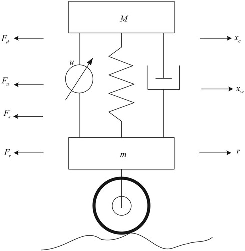
The nonlinear quarter suspension system is shown in Figure 1. $M$ is the spring-loaded mass and is used to represent the vehicle chassis, $m$ is the unsprung mass, indicating the mass of components such as wheels. $u$ as the control input, and $x_c$ denotes the displacement of the spring mass, $x_w$ is the displacement of the unsprung mass, denote the input of road displacement by $r$. $F_d$, $F_s$, $F_u$ and $F_r$ denote the forces applied in the suspension system, respectively, where $F_d$ is generated by the dampers, $F_s$ by the springs, $F_u$ by the actuators, $F_r$ by the disturbances from the road, $k_1$ is the suspension coefficient stiffness, $k_2$ is the damping and $k_3$ is the coefficient of the road disturbance force $F_r$. Then, we can get $F_s=k_1(x_c-x_w)$, $F_d=k_2({\dot{x}}_c-{\dot{x}}_w)$, $F_u=u$ and $F_r=k_3(x_w-r)$.

Figure 1. Quarter suspension system model.

According to Newton’s second law, the resulting dynamic equation is as follow: (1) $\{\begin{array}{l}M{\ddot{x}}_c-F_s-F_d-F_u=0\\ m{\ddot{x}}_w+F_s+F_d+F_u-F_r=0\end{array}$(1)

Then the ideal kinetic equations can be rewritten in the following state space form: (2) $\{\begin{array}{l}{\dot{x}}_c=v_1\\ {\dot{v}}_1=\frac{1}{M}[k_1(x_c-x_w)+k_2({\dot{x}}_c-{\dot{x}}_w)+Ai]\\ {\dot{x}}_w=v_2\\ {\dot{v}}_2=\frac{1}{m}[-k_1(x_c-x_w)-k_2({\dot{x}}_c-{\dot{x}}_w)-Ai+k_3(x_w-r)]\\ \dot{i}=\frac{u-Ri}{L}\\ y=x_c\end{array}$(2)

Define $x_1=x_c,x_2=v_1,x_3=x_w,x_4=v_2$, then, (3) $\{\begin{array}{l}{\dot{x}}_1=x_2\\ {\dot{x}}_2=\frac{1}{M}[k_1(x_1-x_3)+k_2({\dot{x}}_1-{\dot{x}}_3)+Ai]\\ {\dot{x}}_3=x_4\\ {\dot{x}}_4=\frac{1}{m}[-k_1(x_1-x_3)-k_2({\dot{x}}_1-{\dot{x}}_3)-Ai+k_3(x_3-r)]\\ \dot{i}=\frac{u-Ri}{L}\\ y=x_1\end{array}$(3) where $A$ is a constant, $R$ is the resistance and $L$ is the self-inductance factor.

In this paper, the sensor failure considered is partial loss-effectiveness. As stated in Zhang and Yang (2021) and Zhang and Yang (2019), the failure model can be described as, (4) $x_i^f={\rho }_i{x}_i,t\ge T_f$(4) where $0<{\rho }_i\le 1$ denotes the actual output effectiveness of the sensor, $T_f$ is the time constant at which the sensor suffers the partial loss-effectiveness failure.

Control objective: For the nonlinear quarter suspension system Equation (3), design an adaptive fuzzy sensor compensation control scheme. The developed control method can guarantee the closed-loop signals and the tracking performance to be bounded and satisfied, respectively.

3. Sensor failure compensation control design and stability analysis

Step 1: Defining the tracking error of the system as $e_j(j=1,2,3,4)$ and $y_d$ as the tracking signal, according to the definition of sensor faults, we obtain, (5) $\begin{array}{rl}{e}_1& =x_1-y_d\\ & ={\hat{l}}_1{x}_1^f+{\tilde{l}}_1{x}_1^f-y_d\\ & ={\tilde{e}}_1+{\tilde{l}}_1{x}_1^f\end{array}$(5) where ${\hat{l}}_i=l_i-{\tilde{l}}_i$, $l_i=1/{\rho }_i$, ${\hat{l}}_i$ is the estimation of $l_i$.

Then, we can get, (6) ${\dot{e}}_1={\dot{x}}_1-{\dot{y}}_d=x_2-{\dot{y}}_d$(6)

According to the Lyapunov stability theory, the designed Lyapunov function is as follow, (7) $V_1=\frac{1}{2}{e}_1^2+\frac{1}{3{\iota }_1}|{\tilde{l}}_1{|}^3$(7) where ${\iota }_1>0$ is a design parameter.

Then, we can get, (8) ${\dot{V}}_1=e_1{\dot{e}}_1-\frac{1}{{\iota }_1}{\tilde{l}}_1^2{\dot{\hat{l}}}_1\mathrm{sgn}(\tilde{l})$(8)

Substituting ${\dot{e}}_1$ into ${\dot{V}}_1$, one has (9) ${\dot{V}}_1=e_1(x_2-{\dot{y}}_d)-\frac{1}{{\iota }_1}{\tilde{l}}_1^2{\dot{\hat{l}}}_1\mathrm{sgn}(\tilde{l})$(9)

Also, $e_2=x_2-{\alpha }_1$, then (10) ${\dot{V}}_1=e_1(e_2+{\alpha }_1-{\dot{y}}_d)-\frac{1}{{\iota }_1}{\tilde{l}}_1^2{\dot{\hat{l}}}_1\mathrm{sgn}(\tilde{l})$(10)

Design the virtual controller ${\alpha }_1$ as (11) ${\alpha }_1=-{\overline{c}}_1{\tilde{e}}_1+{\dot{y}}_d$(11)

Substituting the virtual controller ${\alpha }_1$ into ${\dot{V}}_1$, we get (12) $\begin{array}{rl}{\dot{V}}_1& =e_1(e_2+{\alpha }_1-{\dot{y}}_d)-\frac{1}{{\iota }_1}{\tilde{l}}_1^2{\dot{\hat{l}}}_1\mathrm{sgn}(\tilde{l})\\ & =-{\overline{c}}_1{e}_1^{}{\tilde{e}}_1+e_1{e}_2-\frac{1}{{\iota }_1}{\tilde{l}}_1^2{\dot{\hat{l}}}_1\mathrm{sgn}({\tilde{l}}_1)\\ & =-{\overline{c}}_1{e}_1^2+\tau ({\overline{c}}_1{\tilde{e}}_1{\tilde{l}}_1{x}_1^f{)}^2+{\overline{c}}_1({\tilde{l}}_1{x}_1^f{)}^2\\ & +\frac{1}{4\tau }+e_1{e}_2-\frac{1}{{\iota }_1}{\tilde{l}}_1^2{\dot{\hat{l}}}_1\mathrm{sgn}({\tilde{l}}_1)\\ & \le -c_1{e}_1^2+\frac{1}{4\tau }+\frac{1}{2}{e}_2^2\\ & +\frac{1}{{\iota }_1}{\tilde{l}}_1^2\mathrm{sgn}({\tilde{l}}_1)({\iota }_1(\tau (c_1{\tilde{e}}_1{)}^2+{\overline{c}}_1)(x_1^f{)}^2-{\dot{\hat{l}}}_1)\end{array}$(12) where $c_1={\overline{c}}_1-\frac{1}{2}>0$ is a design parameter.

Design the parameter adaptive law of ${\hat{l}}_1$ as (13) ${\dot{\hat{l}}}_1=\{\begin{array}{l}{\iota }_1(\tau ({\overline{c}}_1{\tilde{e}}_1{)}^2+{\overline{c}}_1)(x_1^f{)}^2-{\sigma }_1{\hat{l}}_1,p_1\ge 0\\ 0p_1<0\end{array}$(13) where $p_1={\iota }_1(\tau ({\overline{c}}_1{\tilde{e}}_1{)}^2+{\overline{c}}_1)(x_1^f{)}^2-{\sigma }_1{\hat{l}}_1$, and ${\sigma }_1$is a positive design parameter.

Remark 3.1:

It follows from Equation (5) that ${\tilde{e}}_1$ will change quickly when the sensor suffers the lose-effectiveness failure. The change can be utilized to design the adaptive law of ${\hat{l}}_1$ for compensating the failure. The design parameter ${\iota }_1$ should be small enough, and the design parameter $\tau$ should be large enough.

Then, Equation (12) becomes (14) ${\dot{V}}_1\le -c_1{e}_1^2+\frac{1}{2}{e}_2^2+\frac{{\sigma }_1}{{\iota }_1}{\tilde{l}}_1^2{\hat{l}}_1\mathrm{sgn}({\tilde{l}}_1)+D_1$(14)

Step 2: According to the Lyapunov stability theory, the designed Lyapunov function is as follow (15) $V_2=V_1+\frac{M}{2}{e}_2^2+\frac{1}{2}{\tilde{\mathrm{\Theta }}}_2^2+\frac{1}{2}{\tilde{\theta }}_2^T{\tilde{\theta }}_2+\frac{1}{3{\iota }_2}|{\tilde{l}}_2{|}^3$(15) where ${\tilde{\mathrm{\Theta }}}_j={\mathrm{\Theta }}_j^{\ast }-{\mathrm{\Theta }}_j$, ${\tilde{\theta }}_j={\theta }_j^{\ast }-{\theta }_j$, ${\mathrm{\Theta }}_j$ as the estimation of ${\mathrm{\Theta }}_j^{\ast }$, ${\theta }_j$ as the estimation of ${\theta }_j^{\ast }$ and $j=2,3,4,5.$

Then, substituting ${\dot{V}}_1$ into ${\dot{V}}_2$ (16) ${\dot{V}}_2={\dot{V}}_1+M{e}_2{\dot{e}}_2-{\tilde{\mathrm{\Theta }}}_2{\dot{\mathrm{\Theta }}}_2-{\tilde{\theta }}_2^T{\dot{\theta }}_2-\frac{1}{{\iota }_2}{\tilde{l}}_2^2{\dot{\hat{l}}}_2\mathrm{sgn}({\tilde{l}}_2)$(16) where ${\dot{\mathrm{\Theta }}}_j$ and ${\dot{\theta }}_j(j=2,3,4,5)$ are parameter adaptive laws.

Then (17) $\begin{array}{rl}{\dot{e}}_2& ={\dot{x}}_2-{\dot{\alpha }}_1\\ & =\frac{1}{M}[k_1(x_1-x_3)+k_2({\dot{x}}_1-{\dot{x}}_3)+Ai]-{\dot{\alpha }}_1\\ & =\frac{1}{M}[k_1(x_1-x_3)+k_2({\dot{x}}_1-{\dot{x}}_3)+Ai-M{\dot{\alpha }}_1]\end{array}$(17)

Substituting into ${\dot{V}}_2$ yields (18) $\begin{array}{rl}{\dot{V}}_2& ={\dot{V}}_1+M{e}_2{\dot{e}}_2-{\tilde{\mathrm{\Theta }}}_2{\dot{\mathrm{\Theta }}}_2-{\tilde{\theta }}_2^T{\dot{\theta }}_2-\frac{1}{{\iota }_2}{\tilde{l}}_2^2{\dot{\hat{l}}}_2\mathrm{sgn}({\tilde{l}}_2)\\ & +M{e}_2\frac{1}{M}[k_1(x_1-x_3)+k_2({\dot{x}}_1-{\dot{x}}_3)\\ & +Ai-M{\dot{\alpha }}_1]\end{array}$(18)

Using the fuzzy logic system ${\theta }_2^T{\varphi }_2(X_2)$, the unknown quantity $k_1(x_1-x_3)+k_2({\dot{x}}_1-{\dot{x}}_3)+Ai-M{\dot{\alpha }}_1-x_3$ is approximated, where $X_2=(x_1,x_2,x_3,x_4,y_r,{\dot{y}}_r)$for convenience below, we define ${\overline{x}}_j=(x_1,x_2,\dots ,x_j)$, $j=1,2,3,4$, $X_2=({\overline{x}}_4,y_r,{\dot{y}}_r)$. Thus, we obtain (19) $\begin{array}{rl}{\theta }_2^{\ast T}{\varphi }_2(X_2)+{\epsilon }_2(X_2)& =k_1(x_1-x_3)+k_2({\dot{x}}_1-{\dot{x}}_3)\\ & +Ai-M{\dot{\alpha }}_1-x_3\end{array}$(19) Due to ${\tilde{\theta }}_j={\theta }_j^{\ast }-{\theta }_j$, we can obtain that (20) ${\tilde{\theta }}_2^T{\varphi }_2({\overline{x}}_2)={\theta }_2^{\ast T}{\varphi }_2({\overline{x}}_2)-{\theta }_2^T{\varphi }_2({\overline{x}}_2)$(20) Then (21) $\begin{array}{rl}{\dot{V}}_2& ={\dot{V}}_1+e_2[{\theta }_2^T{\varphi }_2({\overline{\hat{l}}}_2,{\overline{x}}_2^f)-{\theta }_2^{\ast T}{\varphi }_2({\overline{\hat{l}}}_2,{\overline{x}}_2^f)+{\tilde{\theta }}_2^T{\varphi }_2({\overline{\hat{l}}}_2,{\overline{x}}_2^f)\\ & +{\theta }_2^{\ast T}{\varphi }_2(X_2)+{\epsilon }_2(X_2)+e_3+{\alpha }_2]\\ & -{\tilde{\mathrm{\Theta }}}_2{\dot{\mathrm{\Theta }}}_2-{\tilde{\theta }}_2^T{\dot{\theta }}_2-\frac{1}{{\iota }_2}{\tilde{l}}_2^2{\dot{\hat{l}}}_2\mathrm{sgn}({\tilde{l}}_2)\end{array}$(21) By using Young’s inequality, one has (22) $\begin{array}{rl}& e_2{\tilde{\theta }}_2^T{\varphi }_2({\overline{\hat{l}}}_2,{\overline{x}}_2^f)\\ & ={\tilde{e}}_2{\tilde{\theta }}_2^T{\varphi }_2({\overline{\hat{l}}}_2,{\overline{x}}_2^f)+{\tilde{l}}_2{x}_2^f{\tilde{\theta }}_2^T{\varphi }_2({\overline{\hat{l}}}_2,{\overline{x}}_2^f)\\ & \le {\tilde{e}}_2{\tilde{\theta }}_2^T{\varphi }_2({\overline{\hat{l}}}_2,{\overline{x}}_2^f)+\tau ({\tilde{l}}_2{x}_2^f{)}^2+\frac{1}{4\tau }{\tilde{\theta }}_2^T{\tilde{\theta }}_2\end{array}$(22) (23) $\begin{array}{rl}& e_2[-{\theta }_2^{\ast T}{\varphi }_2({\overline{\hat{l}}}_2,{\overline{x}}_2^f)+{\theta }_2^{\ast T}{\varphi }_2(X_2)]\\ & =({\tilde{e}}_2+{\tilde{l}}_2{x}_2^f)[-{\theta }_2^{\ast T}{\varphi }_2({\overline{\hat{l}}}_2,{\overline{x}}_2^f)+{\theta }_2^{\ast T}{\varphi }_2(X_2)]\\ & \le 2{\tilde{e}}_2^2{\mathrm{\Theta }}_2^{\ast }+\frac{1}{2}+({\tilde{l}}_2{x}_2^f{)}^2+{\mathrm{\Theta }}_2^{\ast }\\ & =2{\tilde{e}}_2^2{\tilde{\mathrm{\Theta }}}_2^{}+2e_2{\tilde{e}}_2^{}{\mathrm{\Theta }}_2^{}-2{\tilde{l}}_2{x}_2^f{\tilde{e}}_2^{}({\mathrm{\Theta }}_2^{\ast }-{\tilde{\mathrm{\Theta }}}_2^{})\\ & +\frac{1}{2}+({\tilde{l}}_2{x}_2^f{)}^2+{\mathrm{\Theta }}_2^{\ast }\\ & \le 2{\tilde{e}}_2^2{\tilde{\mathrm{\Theta }}}_2^{}+2e_2{\tilde{e}}_2^{}{\mathrm{\Theta }}_2^{}+4\tau ({\tilde{l}}_2{x}_2^f{\tilde{e}}_2^{}{)}^2\\ & +\frac{1}{2\tau }{\mathrm{\Theta }}_2^{\ast 2}+\frac{1}{2\tau }{\tilde{\mathrm{\Theta }}}_2^2+\frac{1}{2}+({\tilde{l}}_2{x}_2^f{)}^2+{\mathrm{\Theta }}_2^{\ast }\end{array}$(23) (24) $\begin{array}{rl}& e_2[{\epsilon }_2(X_2)+e_3]\le e_2^2+\frac{1}{2}{\epsilon }_2^{\ast 2}+\frac{1}{2}{e}_3^2\end{array}$(24)

Where Young’s inequality is: let $p$, $q$ be positive real number satisfying $\frac{1}{p}+\frac{1}{q}=1$, then if $a$, $b$ are nonnegative real numbers, $ab\le \frac{a^p}{p}+\frac{b^q}{q}.$

Remark 3.2:

Since the nonlinear function contains the whole states of the system and the tracking error $e_2$ is not available. The operations Equations (22) and (23) are necessary. Under the operations Equations (22) and (23), the algebraic loop problem can be avoided and the virtual controller and adaptive laws can be designed reasonably.

Substituting Equations (22)–(24) into Equation (21) yields (25) $\begin{array}{rl}{\dot{V}}_2& \le {\dot{V}}_1+e_2({\alpha }_2+{\theta }_2^T{\varphi }_2({\overline{\hat{l}}}_2,{\overline{x}}_2^f)+2{\tilde{e}}_2{\mathrm{\Theta }}_2^{})\\ & +{\tilde{\theta }}_2^T({\tilde{e}}_2{\varphi }_2({\overline{\hat{l}}}_2,{\overline{x}}_2^f)-{\dot{\theta }}_2)\\ & +{\tilde{\mathrm{\Theta }}}_2(2{\tilde{e}}_2^2-{\dot{\mathrm{\Theta }}}_2)+\frac{1}{{\iota }_2}{\tilde{l}}_2^2\mathrm{sgn}\\ & ({\tilde{l}}_2)({\iota }_2(4\tau ({\tilde{e}}_2{)}^2+1)(x_2^f{)}^2-{\dot{\hat{l}}}_2)\\ & +e_2^2+\frac{1}{2}{e}_3^2+\frac{1}{2\tau }{\tilde{\mathrm{\Theta }}}_2^2+\frac{1}{4\tau }{\tilde{\theta }}_2^T{\tilde{\theta }}_2\\ & +\frac{1}{2}{\epsilon }_2^{\ast 2}+\frac{1}{2\tau }{\mathrm{\Theta }}_2^{\ast 2}+{\mathrm{\Theta }}_2^{\ast }+\frac{1}{2}\end{array}$(25)

Design the virtual control function ${\alpha }_2$ as (26) ${\alpha }_2=-{\overline{c}}_2{\tilde{e}}_2-{\theta }_2^T{\varphi }_2({\overline{\hat{l}}}_2,{\overline{x}}_2^f)-2{\tilde{e}}_2{\mathrm{\Theta }}_2^{}$(26)

Then, Equation (25) can be written as (27) $\begin{array}{rl}& {\dot{V}}_2\le {\dot{V}}_1-{\overline{c}}_2{e}_2^2+{\tilde{\theta }}_2^T({\tilde{e}}_2{\varphi }_2({\overline{\hat{l}}}_2,{\overline{x}}_2^f)-{\dot{\theta }}_2)+{\tilde{\mathrm{\Theta }}}_2(2{\tilde{e}}_2^2-{\dot{\mathrm{\Theta }}}_2)\\ & +\frac{1}{{\iota }_2}{\tilde{l}}_2^2\mathrm{sgn}({\tilde{l}}_2)({\iota }_2(4\tau ({\tilde{e}}_2{)}^2+\tau ({\overline{c}}_2{\tilde{e}}_2{)}^2\\ & +{\overline{c}}_2+1)(x_2^f{)}^2-{\dot{\hat{l}}}_2)\\ & +e_2^2+\frac{1}{2}{e}_3^2+\frac{1}{2\tau }{\tilde{\mathrm{\Theta }}}_2^2+\frac{1}{4\tau }{\tilde{\theta }}_2^T{\tilde{\theta }}_2\\ & +\frac{1}{2}{\epsilon }_2^{\ast 2}+\frac{1}{2\tau }{\mathrm{\Theta }}_2^{\ast 2}+{\mathrm{\Theta }}_2^{\ast }+\frac{1}{2}\end{array}$(27)

Design the parameter adaptive laws as (28) $\begin{array}{rl}{\dot{\theta }}_2& ={\tilde{e}}_2{\varphi }_2({\overline{\hat{l}}}_2,{\overline{x}}_2^f)-{\lambda }_2{\theta }_2\end{array}$(28) (29) $\begin{array}{rl}{\dot{\mathrm{\Theta }}}_2& =2{\tilde{e}}_2^2-{\overline{\lambda }}_2{\mathrm{\Theta }}_2\end{array}$(29) (30) $\begin{array}{rl}{\dot{\hat{l}}}_2& =\{\begin{array}{l}{\iota }_2(4\tau ({\tilde{e}}_2{)}^2+\tau ({\overline{c}}_2{\tilde{e}}_2{)}^2+{\overline{c}}_2+1)\\ (x_2^f{)}^2-{\sigma }_2{\hat{l}}_2{p}_2\ge 0\\ 0p_2<0\end{array}\end{array}$(30) where $p_2={\iota }_2(4\tau ({\tilde{e}}_2{)}^2+\tau ({\overline{c}}_2{\tilde{e}}_2{)}^2+{\overline{c}}_2+1)(x_2^f{)}^2-{\sigma }_2{\hat{l}}_2$, ${\lambda }_2$, ${\overline{\lambda }}_2$ and ${\sigma }_2$ are positive design parameters.

Substituting Equations (28)–(30) into Equation (27) yields (31) $\begin{array}{rl}{\dot{V}}_2& \le -\sum _{i=1}^2{\overline{c}}_i{e}_i^2+{\lambda }_2{\tilde{\theta }}_2^T{\theta }_2+{\overline{\lambda }}_2{\tilde{\mathrm{\Theta }}}_2{\mathrm{\Theta }}_2+\sum _{i=1}^2\frac{{\sigma }_i}{{\iota }_i}{\tilde{l}}_i^2\mathrm{sgn}({\tilde{l}}_i){\hat{l}}_i\\ & +\frac{1}{2}{e}_3^2+\frac{1}{2\tau }{\tilde{\mathrm{\Theta }}}_2^2+\frac{1}{4\tau }{\tilde{\theta }}_2^T{\tilde{\theta }}_2+D_2\end{array}$(31) where $c_2={\overline{c}}_2-\frac{3}{2}>0$ is a design parameter, and $D_2=D_1+\frac{1}{2}{\epsilon }_2^{\ast 2}+\frac{1}{2\tau }{\mathrm{\Theta }}_2^{\ast 2}+{\mathrm{\Theta }}_2^{\ast }+\frac{1}{2}$.

Step 3: According to the Lyapunov stability theory, the designed Lyapunov function is as follows (32) $V_3=V_2+\frac{1}{2}{e}_3^2+\frac{1}{2}{\tilde{\theta }}_3^T{\tilde{\theta }}_3+\frac{1}{3{\iota }_3}|{\tilde{l}}_3{|}^3$(32)

Similarly, we can get (33) ${\dot{V}}_3={\dot{V}}_2+e_3{\dot{e}}_3-{\tilde{\theta }}_3^T{\dot{\theta }}_3-\frac{1}{{\iota }_3}{\tilde{l}}_3^2{\dot{\hat{l}}}_3\mathrm{sgn}({\tilde{l}}_3)$(33) Then (34) ${\dot{V}}_3={\dot{V}}_2+e_3{\dot{e}}_3-{\tilde{\theta }}_3^T{\dot{\theta }}_3-\frac{1}{{\iota }_3}{\tilde{l}}_3^2{\dot{\hat{l}}}_3\mathrm{sgn}({\tilde{l}}_3)$(34)

Taking the derivative of $e_3$, we get (35) ${\dot{e}}_3={\dot{x}}_3-{\dot{\alpha }}_2=x_4-{\dot{\alpha }}_2$(35) Then (36) ${\dot{V}}_3={\dot{V}}_2+e_3(x_4-{\dot{\alpha }}_2)-{\tilde{\theta }}_3^T{\dot{\theta }}_3-\frac{1}{{\iota }_3}{\tilde{l}}_3^2{\dot{\hat{l}}}_3\mathrm{sgn}({\tilde{l}}_3)$(36)

Approximation of $-{\dot{\alpha }}_2$ using fuzzy logic system ${\theta }_3^T{\varphi }_3(X_3)$ yields (37) ${\theta }_3^{\ast T}{\varphi }_3(X_3)+{\epsilon }_3(X_3)=-{\dot{\alpha }}_2$(37) where $X_3=({\overline{\hat{l}}}_2,{\overline{x}}_2^f,y_r,{\dot{y}}_r,{\ddot{y}}_r,{\theta }_2,{\mathrm{\Theta }}_2).$

Then (38) $\begin{array}{rl}& {\dot{V}}_3\\ & ={\dot{V}}_2+e_3(e_4+{\alpha }_3+{\theta }_3^T{\varphi }_3(X_3)+{\tilde{\theta }}_3^T{\varphi }_3(X_3)+{\epsilon }_3(X_3))\\ & -{\tilde{\theta }}_3^T{\dot{\theta }}_3-\frac{1}{{\iota }_3}{\tilde{l}}_3^2{\dot{\hat{l}}}_3\mathrm{sgn}({\tilde{l}}_3)\end{array}$(38)

Based on Young’s inequality, one obtains (39) $\begin{array}{rl}& e_3(e_4+{\tilde{\theta }}_3^T{\varphi }_3(X_3)+{\epsilon }_3(X_3))\\ & \le e_3^2+\frac{1}{2}{e}_4^2+\frac{1}{2}{\epsilon }_3^{\ast 2}+{\tilde{e}}_3{\tilde{\theta }}_3^T{\varphi }_3(X_3)+{\tilde{l}}_3{x}_3^f{\tilde{\theta }}_3^T{\varphi }_3(X_3)\\ & \le e_3^2+\frac{1}{2}{e}_4^2+\frac{1}{2}{\epsilon }_3^{\ast 2}+{\tilde{e}}_3{\tilde{\theta }}_3^T{\varphi }_3(X_3)+\frac{1}{2}({\tilde{l}}_3{x}_3^f{)}^2+\frac{1}{2}{\tilde{\theta }}_3^T{\tilde{\theta }}_3\end{array}$(39)

Combining Equations (38) and (39), it can be shown that (40) $\begin{array}{rl}{\dot{V}}_3& \le {\dot{V}}_2+e_3({\alpha }_3+{\theta }_3^T{\varphi }_3(X_3))\\ & +e_3^2+\frac{1}{2}{e}_4^2+\frac{1}{2}{\epsilon }_3^{\ast 2}+\frac{1}{2}{\tilde{\theta }}_3^T{\tilde{\theta }}_3\\ & +{\tilde{\theta }}_3^T({\tilde{e}}_3{\varphi }_3(X_3)-{\dot{\theta }}_3)+\frac{1}{{\iota }_3}{\tilde{l}}_3^2\mathrm{sgn}({\tilde{l}}_3)({\iota }_3(x_3^f{)}^2-{\dot{\hat{l}}}_3)\end{array}$(40)

The design virtual control function ${\alpha }_3$ as (41) ${\alpha }_3=-{\overline{c}}_3{\tilde{e}}_3-{\theta }_3^T{\varphi }_3(X_3)$(41)

Then, Equation (40) becomes (42) $\begin{array}{rl}{\dot{V}}_3& \le {\dot{V}}_2-c_3{e}_3^2+\frac{1}{2}{e}_4^2+\frac{1}{2}{\epsilon }_3^{\ast 2}\\ & +\frac{1}{2}{\tilde{\theta }}_3^T{\tilde{\theta }}_3+{\tilde{\theta }}_3^T({\tilde{e}}_3{\varphi }_3(X_3)-{\dot{\theta }}_3)\\ & +\frac{1}{{\iota }_3}{\tilde{l}}_3^2\mathrm{sgn}({\tilde{l}}_3)({\iota }_3(\tau ({\overline{c}}_3{\tilde{e}}_3{)}^2+{\overline{c}}_3+1)(x_3^f{)}^2-{\dot{\hat{l}}}_3)\end{array}$(42) where $c_3={\overline{c}}_3-\frac{3}{2}>0$ is a design parameter.

Design the parameter adaptive laws as (43) $\begin{array}{rl}{\dot{\theta }}_3& ={\tilde{e}}_3{\varphi }_3(X_3)-{\lambda }_3{\theta }_3\end{array}$(43) (44) $\begin{array}{rl}{\dot{\hat{l}}}_3& =\{\begin{array}{l}{\iota }_3(\tau ({\overline{c}}_3{\tilde{e}}_3{)}^2+{\overline{c}}_3+1)(x_3^f{)}^2-{\sigma }_3{\hat{l}}_3{p}_3\ge 0\\ 0p_3<0\end{array}\end{array}$(44) where $p_3={\iota }_3(\tau ({\overline{c}}_3{\tilde{e}}_3{)}^2+{\overline{c}}_3+1)(x_3^f{)}^2-{\sigma }_3{\hat{l}}_3$, ${\lambda }_3$ and ${\sigma }_3$ are positive design parameters.

Substituting Equations (43) and (44) into Equation (42) yields (45) $\begin{array}{rl}{\dot{V}}_3& \le -\sum _{i=1}^3{\overline{c}}_i{e}_i^2+\sum _{i=2}^3{\lambda }_i{\tilde{\theta }}_i^T{\theta }_i+{\overline{\lambda }}_2{\tilde{\mathrm{\Theta }}}_2{\mathrm{\Theta }}_2\\ & +\sum _{i=1}^3\frac{{\sigma }_i}{{\iota }_i}{\tilde{l}}_i^2\mathrm{sgn}({\tilde{l}}_i){\hat{l}}_i\\ & +\frac{1}{2}{e}_4^2+\frac{1}{2}{\tilde{\theta }}_3^T{\tilde{\theta }}_3+\frac{1}{2\tau }{\tilde{\mathrm{\Theta }}}_2^2+\frac{1}{4\tau }{\tilde{\theta }}_2^T{\tilde{\theta }}_2+D_{\text{3}}\end{array}$(45) where $D_{\text{3}}=D_{\text{2}}+\frac{1}{2}{\epsilon }_3^{\ast 2}.$

Step 4: According to the Lyapunov stability theory, the designed Lyapunov function is as follows: (46) $V_4=V_3+\frac{m}{2}{e}_4^2+\frac{1}{2}{\tilde{\mathrm{\Theta }}}_4^2+\frac{1}{2}{\tilde{\theta }}_4^T{\tilde{\theta }}_4+\frac{1}{3{\iota }_4}|{\tilde{l}}_4{|}^3$(46) Then (47) ${\dot{V}}_4={\dot{V}}_3+m{e}_4{\dot{e}}_4-{\tilde{\mathrm{\Theta }}}_4{\dot{\mathrm{\Theta }}}_4-{\tilde{\theta }}_4^T{\dot{\theta }}_4-\frac{1}{{\iota }_4}{\tilde{l}}_4^2{\dot{\hat{l}}}_4\mathrm{sgn}({\tilde{l}}_4)$(47)

Derivation of $e_4$ yields (48) $\begin{array}{rl}{\dot{e}}_4& ={\dot{x}}_4-{\dot{\alpha }}_3\\ & =\frac{1}{m}[-k_1(x_1-x_3)-k_2({\dot{x}}_1-{\dot{x}}_3)\\ & -Ai+k_3(x_3-r)-m{\dot{\alpha }}_3]\end{array}$(48)

Substituting ${\dot{e}}_4$ into ${\dot{V}}_4$ yields (49) $\begin{array}{rl}{\dot{V}}_4& ={\dot{V}}_3+e_4[-k_1(x_1-x_3)-k_2({\dot{x}}_1-{\dot{x}}_3)-Ai\\ & +k_3(x_3-r)-m{\dot{\alpha }}_3]\\ & -{\tilde{\mathrm{\Theta }}}_4{\dot{\mathrm{\Theta }}}_4-{\tilde{\theta }}_4^T{\dot{\theta }}_4-\frac{1}{{\iota }_4}{\tilde{l}}_4^2{\dot{\hat{l}}}_4\mathrm{sgn}({\tilde{l}}_4)\end{array}$(49) By using the fuzzy logic system ${\theta }_4^T{\varphi }_4(X_4)$ to approximate $-k_1(x_1-x_3)-k_2({\dot{x}}_1-{\dot{x}}_3)+k_3(x_3-r)-m{\dot{\alpha }}_3-Ai-i,$ we obtain (50) $\begin{array}{r}{\theta }_4^{\ast T}{\varphi }_4(X_4)+{\epsilon }_4(X_4)=-k_1(x_1-x_3)-k_2({\dot{x}}_1-{\dot{x}}_3)\\ +k_3(x_3-r)-m{\dot{\alpha }}_3-Ai-i\end{array}$(50) where $X_4=({\overline{x}}_5^{},y_r,{\dot{y}}_r,{\ddot{y}}_r,{\stackrel{⃛}{y}}_r,{\theta }_2,{\theta }_3,{\mathrm{\Theta }}_2).$

Substituting the approximation function into ${\dot{V}}_4$ yields (51) $\begin{array}{rl}{\dot{V}}_4& ={\dot{V}}_4+e_4[e_5+{\alpha }_4+{\theta }_4^T{\phi }_4({\overline{\hat{l}}}_4,{\overline{x}}_4^f)\\ & -{\theta }_4^{\ast T}{\phi }_4({\overline{\hat{l}}}_4,{\overline{x}}_4^f)+{\tilde{\theta }}_4^T{\phi }_4({\overline{\hat{l}}}_4,{\overline{x}}_4^f)\\ & +{\theta }_4^{\ast T}{\phi }_4(X_4)+{\epsilon }_4(X_4)]-{\tilde{\mathrm{\Theta }}}_4{\dot{\mathrm{\Theta }}}_4-{\tilde{\theta }}_4^T{\dot{\theta }}_4\\ & -\frac{1}{{\iota }_4}{\tilde{l}}_4^2{\dot{\hat{l}}}_4\mathrm{sgn}({\tilde{l}}_4)\end{array}$(51) Based on Young’s inequality and the fact ${\varphi }^T(\cdot )\varphi (\cdot )\le 1,$ one obtains (52) $\begin{array}{rl}& e_4{\tilde{\theta }}_4^T{\varphi }_4({\overline{\hat{l}}}_4,{\overline{x}}_4^f)\\ & ={\tilde{e}}_4{\tilde{\theta }}_4^T{\varphi }_4({\overline{\hat{l}}}_4,{\overline{x}}_4^f)+{\tilde{l}}_4{x}_4^f{\tilde{\theta }}_4^T{\varphi }_4({\overline{\hat{l}}}_4,{\overline{x}}_4^f)\\ & \le {\tilde{e}}_4{\tilde{\theta }}_4^T{\varphi }_4({\overline{\hat{l}}}_4,{\overline{x}}_4^f)+\tau ({\tilde{l}}_4{x}_4^f{)}^2+\frac{1}{4\tau }{\tilde{\theta }}_4^T{\tilde{\theta }}_4\end{array}$(52) (53) $\begin{array}{rl}& e_4[-{\theta }_4^{\ast T}{\varphi }_4({\overline{\hat{l}}}_4,{\overline{x}}_4^f)+{\theta }_4^{\ast T}{\varphi }_4(X_4)]\\ & =({\tilde{e}}_4+{\tilde{l}}_4{x}_4^f)[-{\theta }_4^{\ast T}{\varphi }_4({\overline{\hat{l}}}_4,{\overline{x}}_4^f)+{\theta }_4^{\ast T}{\varphi }_4(X_4)]\\ & \le 2{\tilde{e}}_4^2{\mathrm{\Theta }}_4^{\ast }+\frac{1}{2}+({\tilde{l}}_4{x}_4^f{)}^2+{\mathrm{\Theta }}_4^{\ast }\\ & =2{\tilde{e}}_4^2{\tilde{\mathrm{\Theta }}}_4^{}+2e_4{\tilde{e}}_4^{}{\mathrm{\Theta }}_4^{}-2{\tilde{l}}_4{x}_4^f{\tilde{e}}_4^{}({\mathrm{\Theta }}_4^{\ast }-{\tilde{\mathrm{\Theta }}}_4^{})\\ & +\frac{1}{2}+({\tilde{l}}_4{x}_4^f{)}^2+{\mathrm{\Theta }}_4^{\ast }\\ & \le 2{\tilde{e}}_4^2{\tilde{\mathrm{\Theta }}}_4^{}+2e_4{\tilde{e}}_4^{}{\mathrm{\Theta }}_4^{}+4\tau ({\tilde{l}}_4{x}_4^f{\tilde{e}}_4^{}{)}^2+\frac{1}{2\tau }{\mathrm{\Theta }}_4^{\ast 2}\\ & +\frac{1}{2\tau }{\tilde{\mathrm{\Theta }}}_4^2+\frac{1}{2}+({\tilde{l}}_4{x}_4^f{)}^2+{\mathrm{\Theta }}_4^{\ast }\end{array}$(53) (54) $\begin{array}{rl}& e_4[{\epsilon }_4(X_4)+e_5]\\ & \le e_4^2+\frac{1}{2}{\epsilon }_4^{\ast 2}+\frac{1}{2}{e}_5^2\end{array}$(54)

Substituting Equations (52)–(54) into Equation (51) yields (55) $\begin{array}{rl}{\dot{V}}_4& \le {\dot{V}}_3+e_4({\alpha }_4+{\theta }_4^T{\varphi }_4({\overline{\hat{l}}}_4,{\overline{x}}_4^f)+2{\tilde{e}}_4{\mathrm{\Theta }}_4^{})\\ & +{\tilde{\theta }}_4^T({\tilde{e}}_4{\varphi }_4({\overline{\hat{l}}}_4,{\overline{x}}_4^f)-{\dot{\theta }}_4)\\ & +{\tilde{\mathrm{\Theta }}}_4(2{\tilde{e}}_4^2-{\dot{\mathrm{\Theta }}}_4)+\frac{1}{{\iota }_4}{\tilde{l}}_4^2\mathrm{sgn}({\tilde{l}}_4)\\ & ({\iota }_4(4\tau ({\tilde{e}}_4{)}^2+1)(x_4^f{)}^2-{\dot{\hat{l}}}_4)\\ & +e_4^2+\frac{1}{2}{e}_5^2+\frac{1}{2\tau }{\tilde{\mathrm{\Theta }}}_4^2+\frac{1}{4\tau }{\tilde{\theta }}_4^T{\tilde{\theta }}_4\\ & +\frac{1}{2}{\epsilon }_4^{\ast 2}+\frac{1}{2\tau }{\mathrm{\Theta }}_4^{\ast 2}+{\mathrm{\Theta }}_4^{\ast }+\frac{1}{2}\end{array}$(55)

Design controller $\alpha {}_4$ as (56) ${\alpha }_4=-{\overline{c}}_4{\tilde{e}}_4-{\theta }_4^T{\varphi }_4({\overline{\hat{l}}}_4,{\overline{x}}_4^f)-2{\tilde{e}}_4{\mathrm{\Theta }}_4^{}$(56)

Then, Equation (55) becomes (57) $\begin{array}{rl}{\dot{V}}_4& \le {\dot{V}}_3-{\overline{c}}_4{e}_4^2+{\tilde{\theta }}_4^T({\tilde{e}}_4{\varphi }_4({\overline{\hat{l}}}_4,{\overline{x}}_4^f)-{\dot{\theta }}_4)+{\tilde{\mathrm{\Theta }}}_4(2{\tilde{e}}_4^2-{\dot{\mathrm{\Theta }}}_4)\\ & +\frac{1}{{\iota }_4}{\tilde{l}}_4^2\mathrm{sgn}({\tilde{l}}_4)\\ & ({\iota }_4(4\tau ({\tilde{e}}_4{)}^2+\tau ({\overline{c}}_4{\tilde{e}}_4{)}^2+{\overline{c}}_4+1)(x_4^f{)}^2-{\dot{\hat{l}}}_4)\\ & +e_4^2+\frac{1}{2}{e}_5^2+\frac{1}{2\tau }{\tilde{\mathrm{\Theta }}}_4^2\\ & +\frac{1}{4\tau }{\tilde{\theta }}_4^T{\tilde{\theta }}_4+\frac{1}{2}{\epsilon }_4^{\ast 2}+\frac{1}{2\tau }{\mathrm{\Theta }}_4^{\ast 2}+{\mathrm{\Theta }}_4^{\ast }+\frac{1}{2}\end{array}$(57)

The design parameter adaptive laws are designed as (58) $\begin{array}{rl}{\dot{\theta }}_4& ={\tilde{e}}_4{\varphi }_4({\overline{\hat{l}}}_4,{\overline{x}}_4^f)-{\lambda }_4{\theta }_4\end{array}$(58) (59) $\begin{array}{rl}{\dot{\mathrm{\Theta }}}_4& =2{\tilde{e}}_4^2-{\overline{\lambda }}_4{\mathrm{\Theta }}_4\end{array}$(59) (60) $\begin{array}{rl}{\dot{\hat{l}}}_4& =\{\begin{array}{l}{\iota }_4(4\tau ({\tilde{e}}_4{)}^2+\tau ({\overline{c}}_4{\tilde{e}}_4{)}^2+{\overline{c}}_4+1)\\ (x_4^f{)}^2-{\sigma }_4{\hat{l}}_4{p}_4\ge 0\\ 0p_4<0\end{array}\end{array}$(60) where $p_4={\iota }_4(4\tau ({\tilde{e}}_4{)}^2+\tau ({\overline{c}}_4{\tilde{e}}_4{)}^2+{\overline{c}}_4+1)(x_4^f{)}^2-{\sigma }_4{\hat{l}}_4$, ${\lambda }_4$, ${\overline{\lambda }}_4$ and${\sigma }_4$ are positive design parameters.

Substituting Equations (58)–(60) into Equation (57) yields (61) $\begin{array}{rl}{\dot{V}}_4& \le -\sum _{i=1}^4{\overline{c}}_i{e}_i^2+\sum _{i=2}^4{\lambda }_i{\tilde{\theta }}_i^T{\theta }_i+{\overline{\lambda }}_2{\tilde{\mathrm{\Theta }}}_2{\mathrm{\Theta }}_2+{\overline{\lambda }}_4{\tilde{\mathrm{\Theta }}}_4{\mathrm{\Theta }}_4\\ & +\sum _{i=1}^4\frac{{\sigma }_i}{{\iota }_i}{\tilde{l}}_i^2\mathrm{sgn}({\tilde{l}}_i){\hat{l}}_i\\ & +\frac{1}{2}{e}_5^2+\frac{1}{2\tau }{\tilde{\mathrm{\Theta }}}_4^2+\frac{1}{4\tau }{\tilde{\theta }}_4^T{\tilde{\theta }}_4+\frac{1}{2}{\tilde{\theta }}_3^T{\tilde{\theta }}_3\\ & +\frac{1}{2\tau }{\tilde{\mathrm{\Theta }}}_2^2+\frac{1}{4\tau }{\tilde{\theta }}_2^T{\tilde{\theta }}_2+D_4\end{array}$(61) where $c_4={\overline{c}}_4-\frac{3}{2}>0$ is a design parameter, and $D_4=D_3++\frac{1}{2}{\epsilon }_4^{\ast 2}+\frac{1}{2\tau }{\mathrm{\Theta }}_4^{\ast 2}+{\mathrm{\Theta }}_4^{\ast }+\frac{1}{2}.$

Step 5: According to Lyapunov stability theory, the following Lyapunov function $V_5$ is designed. (62) $V_5=V_4+\frac{1}{2}{e}_5^2+\frac{1}{2}{\tilde{\theta }}_5^T{\tilde{\theta }}_5+\frac{1}{3{\iota }_5}|{\tilde{l}}_5{|}^3$(62) Then (63) ${\dot{V}}_5={\dot{V}}_4+e_5{\dot{e}}_5-{\tilde{\theta }}_5^T{\dot{\theta }}_5-\frac{1}{{\iota }_5}{\tilde{l}}_5^2{\dot{\hat{l}}}_5\mathrm{sgn}({\tilde{l}}_5)$(63) Derive $e_5$ to obtain ${\dot{e}}_5$ (64) ${\dot{e}}_5=\dot{i}-{\dot{\alpha }}_4=\frac{u-Ri}{L}-{\dot{\alpha }}_4$(64) Then (65) ${\dot{V}}_5={\dot{V}}_4+e_5(\frac{u-Ri}{L}-{\dot{\alpha }}_4)-{\tilde{\theta }}_5^T{\dot{\theta }}_5-\frac{1}{{\iota }_5}{\tilde{l}}_5^2{\dot{\hat{l}}}_5\mathrm{sgn}({\tilde{l}}_5)$(65)

Using the fuzzy logic system ${\theta }_5^T{\varphi }_5(X_5)$ to approximate $-Ri/L-{\dot{\alpha }}_4$, we obtain (66) ${\theta }_5^{\ast T}{\varphi }_5(X_5)+{\epsilon }_5(X_5)=-\frac{Ri}{L}-{\dot{\alpha }}_4$(66) where $X_5=({\overline{x}}_5^f,{\hat{\overline{l}}}_5,y_r,\dots ,y_r^{(4)},{\theta }_2,{\theta }_3,{\theta }_4,{\mathrm{\Theta }}_2,{\mathrm{\Theta }}_4)$.

Then (67) $\begin{array}{rl}{\dot{V}}_5& ={\dot{V}}_4+e_5\frac{u}{L}+e_5({\theta }_5^T{\varphi }_5(X_5)+{\tilde{\theta }}_5^T{\varphi }_5(X_5)\\ & +{\epsilon }_5(X_5))-{\tilde{\theta }}_5^T{\dot{\theta }}_5-\frac{1}{{\iota }_5}{\tilde{l}}_5^2{\dot{\hat{l}}}_5\mathrm{sgn}({\tilde{l}}_5)\end{array}$(67)

Based on Young’s inequality and the fact ${\varphi }^T(\cdot )\varphi (\cdot )\le 1$, one obtains (68) $\begin{array}{rl}& e_5({\tilde{\theta }}_5^T{\varphi }_5(X_5)+{\epsilon }_5(X_5))\\ & =({\tilde{e}}_5+{\tilde{l}}_5{x}_5^f){\tilde{\theta }}_5^T{\varphi }_5(X_5)+e_5{\epsilon }_5(X_5)\\ & \le {\tilde{e}}_5{\tilde{\theta }}_5^T{\varphi }_5(X_5)\\ & +\frac{1}{2}({\tilde{l}}_5{x}_5^f{)}^2+\frac{1}{2}{\tilde{\theta }}_5^T{\tilde{\theta }}_5+\frac{1}{2}{e}_5^2+\frac{1}{2}{\epsilon }_5^{\ast 2}\end{array}$(68)

Substitute Equation (68) into Equation (67) yields (69) $\begin{array}{rl}& {\dot{V}}_5\le {\dot{V}}_4+e_5+e_5(\frac{u}{L}+{\theta }_5^T{\varphi }_5(X_5))+{\tilde{\theta }}_5^T({\tilde{e}}_5{\varphi }_5(X_5)-{\dot{\theta }}_5)\\ & +\frac{1}{{\iota }_5}{\tilde{l}}_5^2\mathrm{sgn}({\tilde{l}}_5)(\frac{l_5}{2}(x_5^f{)}^2-{\dot{\hat{l}}}_5)+\frac{1}{2}{\tilde{\theta }}_5^T{\tilde{\theta }}_5+\frac{1}{2}{e}_5^2+\frac{1}{2}{\epsilon }_5^{\ast 2}\end{array}$(69)

Design controller $u$ as (70) $u=-L({\overline{c}}_5{\tilde{e}}_5+{\theta }_5^T{\varphi }_5(X_5))$(70)

Combining Equations (69) and (70), it can be shown that (71) $\begin{array}{rl}& {\dot{V}}_5\le {\dot{V}}_4-c_5{e}_5^2+{\tilde{\theta }}_5^T({\tilde{e}}_5{\phi }_5(X_5)-{\dot{\theta }}_5)\\ & +\frac{1}{{\iota }_5}{\tilde{l}}_5^2\mathrm{sgn}({\tilde{l}}_5)({\iota }_5(\frac{1}{2}+L{\overline{c}}_5\\ & +\tau (L{\overline{c}}_5{\tilde{e}}_5{)}^2)(x_5^f{)}^2-{\dot{\hat{l}}}_5)+\frac{1}{4\tau }+\frac{1}{2}{\tilde{\theta }}_5^T{\tilde{\theta }}_5+\frac{1}{2}{e}_5^2+\frac{1}{2}{\epsilon }_5^{\ast 2}\end{array}$(71)

Design parameter adaptive laws as (72) $\begin{array}{rl}{\dot{\theta }}_5& ={\tilde{e}}_5{\varphi }_5(X_5)-{\lambda }_5{\theta }_5\end{array}$(72) (73) $\begin{array}{rl}{\dot{\hat{l}}}_5& =\{\begin{array}{l}{\iota }_5(\frac{1}{2}+L{\overline{c}}_5+\tau (L{\overline{c}}_5{\tilde{e}}_5{)}^2)(x_5^f{)}^2-{\sigma }_5{\hat{l}}_5{p}_5>0\\ 0p_5\le 0\end{array}\end{array}$(73) where $c_5=L{\overline{c}}_5-\frac{3}{2}>0$, ${\lambda }_5>0$, and ${\sigma }_5>0$ are design parameters, and $p_5={\iota }_5(\frac{1}{2}+L{\overline{c}}_5+\tau (L{\overline{c}}_5{\tilde{e}}_5{)}^2)(x_5^f{)}^2-{\sigma }_5{\hat{l}}_5$.

Substituting Equations (72) and (73) into Equation (71) yields (74) $\begin{array}{rl}{\dot{V}}_5& \le -\sum _{i=1}^5{c}_i{e}_i^2+\sum _{i=2}^5{\lambda }_i{\tilde{\theta }}_i^T{\theta }_i+{\overline{\lambda }}_2{\tilde{\mathrm{\Theta }}}_2{\mathrm{\Theta }}_2+{\overline{\lambda }}_4{\tilde{\mathrm{\Theta }}}_4{\mathrm{\Theta }}_4\\ & +\sum _{i=1}^5\frac{{\sigma }_i}{{\iota }_i}{\tilde{l}}_i^2\mathrm{sgn}({\tilde{l}}_i){\hat{l}}_i\\ & +\frac{1}{2\tau }{\tilde{\mathrm{\Theta }}}_4^2+\frac{1}{4\tau }{\tilde{\theta }}_4^T{\tilde{\theta }}_4+\frac{1}{2}{\tilde{\theta }}_3^T{\tilde{\theta }}_3\\ & +\frac{1}{2\tau }{\tilde{\mathrm{\Theta }}}_2^2+\frac{1}{4\tau }{\tilde{\theta }}_2^T{\tilde{\theta }}_2+\frac{1}{2}{\tilde{\theta }}_5^T{\tilde{\theta }}_5+D_5\end{array}$(74) where $D_5=D_4+\frac{1}{4\tau }+\frac{1}{2}{\epsilon }_5^{\ast 2}$.

Theorem 3.1:

Consider the nonlinear quarter suspension system Equation (3) under the sensor failures, the actual controller is designed as Equation (70), the virtual controllers are designed as Equations (11), (26), (41), and (56), the adaptive laws are designed as Equations (13), (28)–(30), (43), (44), (58)–(60), (72), and (73), the developed control scheme can guarantee that all the signals in the closed-loop system are bounded and the tracking performance is satisfied.

Proof:

By completing the squares, one has (75) ${\tilde{\theta }}_i^T{\theta }_i\le -\frac{1}{2}{\tilde{\theta }}_i^T{\tilde{\theta }}_i+\frac{1}{2}{\theta }_i^{\ast T}{\theta }_i^{\ast }$(75)

According to the definitions of ${\tilde{\theta }}_i$ and ${\tilde{\mathrm{\Theta }}}_i$,${\tilde{\theta }}_i={\theta }_i^{\ast }-{\theta }_i$ and ${\tilde{\mathrm{\Theta }}}_i={\mathrm{\Theta }}_i^{\ast }-{\mathrm{\Theta }}_i$, by using Young’s inequality, we have (76) $\begin{array}{rl}{\tilde{\theta }}_i^T{\theta }_i& ={\tilde{\theta }}_i^T({\theta }_i^{\ast }-{\tilde{\theta }}_i)={\tilde{\theta }}_i^T{\theta }_i^{\ast }-{\tilde{\theta }}_i^T{\tilde{\theta }}_i\le \frac{1}{2}{\theta }_i^{\ast T}{\theta }_i^{\ast }-\frac{1}{2}{\tilde{\theta }}_i^T{\tilde{\theta }}_i\\ {\tilde{\mathrm{\Theta }}}_i{\mathrm{\Theta }}_i& ={\tilde{\mathrm{\Theta }}}_i({\mathrm{\Theta }}_i^{\ast }-{\tilde{\mathrm{\Theta }}}_i)={\tilde{\mathrm{\Theta }}}_i{\mathrm{\Theta }}_i^{\ast }-{\tilde{\mathrm{\Theta }}}_i^2\le \frac{1}{2}{\mathrm{\Theta }}_i^{\ast 2}-\frac{1}{2}{\tilde{\mathrm{\Theta }}}_i^2\\ {\tilde{\mathrm{\Theta }}}_i{\mathrm{\Theta }}_i& \le -\frac{1}{2}{\tilde{\mathrm{\Theta }}}_i^2+\frac{1}{2}{\mathrm{\Theta }}_i^{\ast 2}\end{array}$(76)

Remark 3.3:

As we all known, in the actual situation, the ${\hat{l}}_i(0)$ is usually chosen as 1, and combining with the fact that $\underset{t\to \mathrm{\infty }}{lim}{\hat{l}}_i(t)=l_i$, and ${\hat{l}}_i=l_i-{\tilde{l}}_i$, it can be concluded that the sign of ${\tilde{l}}_i$ is positive.

Then, we have (77) ${\tilde{l}}_i^2\mathrm{sgn}({\tilde{l}}_i){\hat{l}}_i={\tilde{l}}_i^2{\hat{l}}_i\le -\frac{1}{3}|{\tilde{l}}_i{|}^3+\frac{1}{3}{l}_i^3$(77)

Equation (74) can be written as (78) $\begin{array}{rl}\dot{V_5}& \le -\sum _{i=1}^5{c}_i,e_i^2-\sum _{i=2}^5\frac{{\lambda }_i}{2}{\tilde{\theta }}_i^T{\tilde{\theta }}_i^{}-(\frac{{\overline{\lambda }}_2}{2}-\frac{1}{2\tau }){\tilde{\mathrm{\Theta }}}_2^2\\ & -(\frac{{\overline{\lambda }}_4}{2}-\frac{1}{2\tau }){\tilde{\mathrm{\Theta }}}_4^2+\sum _{i=1}^5\frac{{\sigma }_i}{3{\iota }_i}{|{\tilde{l}}_i|}^3\\ & +\frac{1}{2}{\tilde{\theta }}_i^T{\tilde{\theta }}_4+\frac{1}{2}{\tilde{\theta }}_3^T{\tilde{\theta }}_3+\frac{1}{4}{\tilde{\theta }}_2^T{\tilde{\theta }}_2+\frac{1}{2}{\tilde{\theta }}_5^T{\tilde{\theta }}_5+D\end{array}$(78) where $D=D_5+\sum _{i=2}^5\frac{{\lambda }_i}{2}{\theta }_i^{\ast T}{\theta }_i^{\ast }+\frac{{\overline{\lambda }}_2}{2}{\mathrm{\Theta }}_2^{\ast 2}+\frac{{\overline{\lambda }}_4}{2}{\mathrm{\Theta }}_4^{\ast 2}+\sum _{i=1}^5\frac{{\sigma }_i}{3{\iota }_i}{l}_i^3$.

Let $C=min\{2c_i,{\lambda }_2-\frac{1}{2\tau },{\lambda }_3-1,{\lambda }_4-\frac{1}{2\tau },{\lambda }_5-1,{\sigma }_i\}$, $V=V_5$, then (79) $\dot{V}\le -CV+D$(79)

Integrating $\dot{V}$ over the interval $[0,t)$ yields (80) $0\le V(t)\le V(0)e^{-Ct}+\frac{D}{C}$(80)

Therefore, the controller $u$ is bounded, while the tracking error $e_1$ satisfies$|e_1|\le \sqrt{2(V(0)e^{-Ct}+D/C)}$. When we choose appropriate design parameters so that the tracking error is small enough, the error is bounded and the state is also bounded. In addition, the parameter errors ${\tilde{\mathrm{\Theta }}}_j,j=2,4$, ${\tilde{l}}_i,{\tilde{\theta }}_j,j=1,2,3,4,5$ is bounded. Therefore, all signals are bounded. Thus, the proof of the theorem 3.1 has been completed.

4. Simulation

Consider the following quarter active suspension system as (81) $\{\begin{array}{l}{\dot{x}}_1=x_2\\ {\dot{x}}_2=\frac{1}{M}[k_1(x_1-x_3)+k_2({\dot{x}}_1-{\dot{x}}_3)+Ai]\\ {\dot{x}}_3=x_4\\ {\dot{x}}_4=\frac{1}{m}[-k_1(x_1-x_3)-k_2({\dot{x}}_1-{\dot{x}}_3)-Ai+k_3(x_3-r)]\\ \dot{i}=\frac{u-Ri}{L}\\ y=x_1\end{array}$(81)

The system parameters are chosen as: $M=900kg$, $m=100kg$, $k_1=16800N/m$, $k_2=1000N/m$, $k_3=400000N/m$, $L=6H$, $R=1.2\mathrm{\Omega }$ and $A=28$.

In the simulation, the first sensor suffers the 50% loss-effectiveness failure at 10s. The values are chosen as: $[x_1(0),x_2(0),x_3(0),x_4(0),x_5(0){]}^T=[0.1,0,0,0,0{]}^T$, ${\hat{l}}_2(0)=1$, the other values are zeros. The design parameters are chosen as: ${\overline{c}}_1=0.6$, $c_2=1$, $c_3=1$, $c_4=10$, $c_5=22$, ${\iota }_1=0.001$, $\tau =\text{1000}$, ${\sigma }_1=\text{0}\text{.2}$, ${\lambda }_2=1000$, ${\lambda }_3=2000$, ${\lambda }_4=3000$, ${\lambda }_5=3000$, ${\overline{\lambda }}_2=1000$ and ${\overline{\lambda }}_4=2000$. The immediate control signals ${\alpha }_i(i=1,2,3,4)$, actual control signal $u$, the adaptive laws of ${\theta }_i(i=1,2,3,4)$ and ${\mathrm{\Theta }}_i(i=2,4)$ are as follows (82) $\begin{array}{rl}{\alpha }_1& =-{\overline{c}}_1{\tilde{e}}_1+{\dot{y}}_d\end{array}$(82) (83) $\begin{array}{rl}{\dot{\hat{l}}}_1& =\{\begin{array}{l}{\iota }_1(\tau ({\overline{c}}_1{\tilde{e}}_1{)}^2+{\overline{c}}_1)(x_1^f{)}^2-{\sigma }_1{\hat{l}}_1,p_1\ge 0\\ 0p_1<0\end{array}\end{array}$(83) (84) $\begin{array}{rl}{\alpha }_2& =-c_2{e}_2-{\theta }_2^T{\varphi }_2({\overline{x}}_2)-2e_2{\mathrm{\Theta }}_2^{}\end{array}$(84) (85) $\begin{array}{rl}{\dot{\theta }}_2& =e_2{\varphi }_2({\overline{x}}_2)-{\lambda }_2{\theta }_2\end{array}$(85) (86) $\begin{array}{rl}{\dot{\mathrm{\Theta }}}_2& =2e_2^2-{\overline{\lambda }}_2{\mathrm{\Theta }}_2\end{array}$(86) (87) $\begin{array}{rl}{\alpha }_3& =-c_3{e}_3-{\theta }_3^T{\varphi }_3({\overline{x}}_3)\end{array}$(87) (88) $\begin{array}{rl}{\dot{\theta }}_3& =e_3{\varphi }_3({\overline{x}}_3)-{\lambda }_3{\theta }_3\end{array}$(88) (89) $\begin{array}{rl}{\alpha }_4& =-c_4{e}_4-{\theta }_4^T{\varphi }_4({\overline{x}}_4)-2e_4{\mathrm{\Theta }}_4^{}\end{array}$(89) (90) $\begin{array}{rl}{\dot{\theta }}_4& =e_4{\varphi }_4({\overline{x}}_4)-{\lambda }_4{\theta }_4\end{array}$(90) (91) $\begin{array}{rl}{\dot{\mathrm{\Theta }}}_4& =2e_4^2-{\overline{\lambda }}_4{\mathrm{\Theta }}_4\end{array}$(91) (92) $\begin{array}{rl}u& =-L(c_5{e}_5+{\theta }_5^T{\varphi }_5({\overline{x}}_5))\end{array}$(92) (93) $\begin{array}{rl}{\dot{\theta }}_5& =e_5{\varphi }_5({\overline{x}}_5)-{\lambda }_5{\theta }_5\end{array}$(93)

Then, apply the control schemes Equations (82)–(93) into system Equation (81), Figures 2–8 can express the simulation results. Among them, Figure 2 shows the curves of $x_1$ and $y_d$; Figure 3 shows the curve of $x_2$; Figure 4 shows the curve of $x_3$; Figure 5 shows the curve of $x_4$; Figure 6 shows the curve of $x_5$; Figure 7 shows the curve of $u$; Figure 8 shows the curve of $e_i(i=1,2,\dots ,5)$ . Table 1 is a list of all the design parameters.

Figure 2. The curves of $x_1$ and $y_d$.

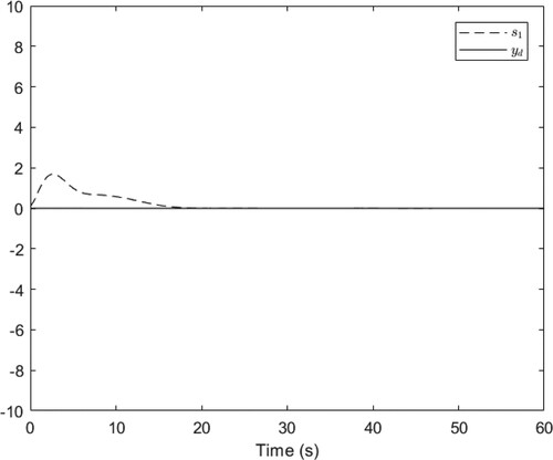
Figure 3. The curve of $x_2$.

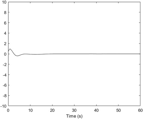
Figure 4. The curve of $x_3$.

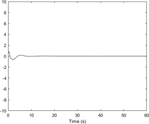
Figure 5. The curve of $x_4$.

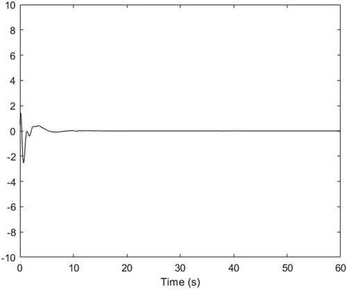
Figure 6. The curve of $x_5$.

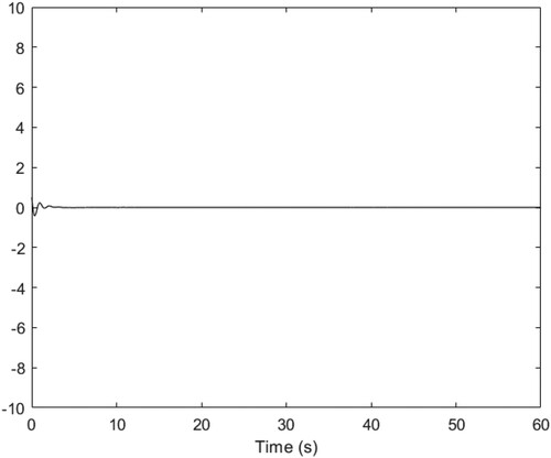
Figure 7. The curve of $u$.

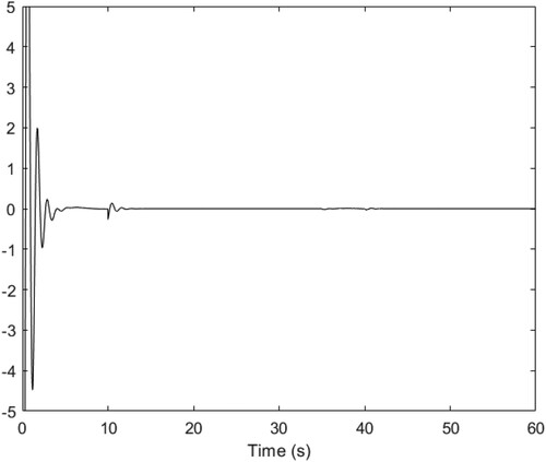
Figure 8. The curves of $e_i(i=1,2,\dots ,5)$.

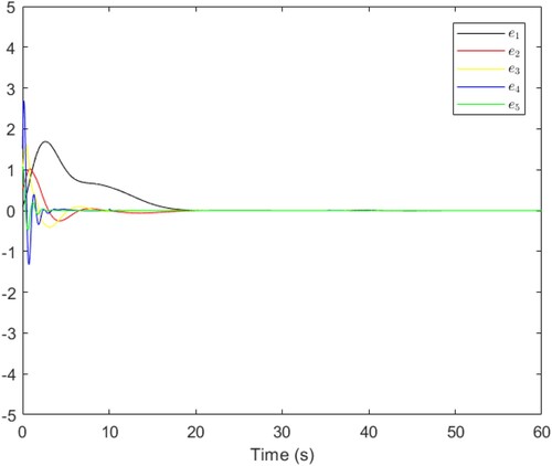
Table 1 Designed parameters.

Figure	Curve
Figure 2	$x_1$ and $y_d$
Figure 3	$x_2$
Figure 4	$x_3$
Figure 5	$x_4$
Figure 6	$x_5$
Figure 7	$u$
Figure 8	$e_i(i=1,2,\dots ,5)$

Remark 4.1:

Calming and tracking issues have different parameter selections in different situations. What has been done here is to track the problem, so we chose $y_d=0$.

Remark 4.2:

A fuzzy logic system is combined with backstepping technique, by this idea, a fault-tolerant control method has been developed. And the proposed control method can guarantee that all the signals in the closed-loop system are all bounded, and the tracking error can converge to the neighbourhood of the origin.

From the above simulation results, it can be shown that all the signals in the closed-loop signals are bounded, and the tracking error can converge to the neighbourhood of the origin. Thus, the developed control scheme can effectively solve the sensor failure compensation control problem of active suspension systems.

5. Conclusion

In this article, a novel sensor failure compensation control method has been studied for active suspension systems. Such designs apply FLSs to approximate the unknown dynamics, utilize the projection technique to compensate the sensor failures. By combining with the backstepping recursive design, a fault-tolerant control scheme has been developed. The developed control scheme can guarantee that all the signals in the closed-loop system are all bounded, and the tracking performance is satisfied. The simulation further verifies the effectiveness of the developed control scheme.

The future study direction will extend the developed control method in this paper to active suspension systems with multiple sensor failures and stochastic disturbance.

Disclosure statement

No potential conflict of interest was reported by the author(s).

Data availability statement

Due to the nature of this research, participants of this study did not agree for their data to be shared publicly, so supporting data is not available.

Additional information

Funding

This work was supported in part by the National Natural Science Foundation of China under Grants 61773189, the Program for Liaoning Innovative Talent in University under Grant LR2019033, the Joint fund of Science & Technology Department of Liaoning Province and State Key Laboratory of Robotics , China under Grants 2020-KF-12-10 and the Foundation of Liaoning Province under Grant 2020JH6/10500050.

References

- Chen, H., & Guo, K.-H. (2005). Constrained control of active suspensions: An LMI approach. IEEE Transactions on Control Systems Technology, 13(3), 412–421. https://doi.org/10.1109/TCST.2004.841661
- Gao, H., Sun, W., & Shi, P. (2010). Robust sampled-data control for vehicle active suspension systems. IEEE Transactions on Control Systems Technology, 18(1), 238–245. https://doi.org/10.1109/TCST.2009.2015653
- Li, H., Zhang, Z., Yan, H., & Xie, X. (2019). Adaptive event-triggered fuzzy control for uncertain active suspension systems. IEEE Transactions on Cybernetics, 49(12), 4388–4397. https://doi.org/10.1109/TCYB.2018.2864776
- Li, H. Y., Jing, X., Lam, H.-K., & Shi, P. (2014). Fuzzy sampled-data control for uncertain vehicle suspension systems. IEEE Transactions on Cybernetics, 44(7), 1111–1126. https://doi.org/10.1109/TCYB.2013.2279534
- Li, K. W., & Li, Y. M. (2021). Fuzzy adaptive optimal consensus fault-tolerant control for stochastic nonlinear multi-agent systems. IEEE Transactions on Fuzzy Systems. https://doi.org/10.1007/s12555-018-0751-0
- Li, Y. X., Wang, Q. Y., & Tong, S. C. (2021). Fuzzy adaptive fault-tolerant control of fractional-order nonlinear systems. IEEE Transactions on Systems, 51(10), 1372–1379. https://doi.org/10.1109/TSMC.2019.2894663
- Liu, B., Saif, M., & Fan, H. (2016). Adaptive fault tolerant control of a half-car active suspension systems subject to random actuator failures. IEEE/ASME Transactions on Mechatronics, 21(6), 2847–2857. https://doi.org/10.1109/TMECH.2016.2587159
- Liu, L., Liu, Y.-J., & Tong, S. (2019). Neural networks-based adaptive finite-time fault-tolerant control for a class of strict-feedback switched nonlinear systems. IEEE Transactions on Cybernetics, 49(7), 2536–2545. https://doi.org/10.1109/TCYB.2018.2828308
- Liu, L., Wang, Z., & Zhang, H. (2017). Adaptive fault-tolerant tracking control for MIMO discrete-time systems via reinforcement learning algorithm with less learning parameters. IEEE Transactions on Automation Science and Engineering, 14(1), 299–313. https://doi.org/10.1109/TASE.2016.2517155
- Liu, Y.-J., Zeng, Q., Tong, S., Chen, C. L. P., & Liu, L. (2019). Adaptive neural network control for active suspension systems with time-varying vertical displacement and speed constraints. IEEE Transactions on Industrial Electronics, 66(12), 9458–9466. https://doi.org/10.1109/TIE.2019.2893847
- Liu, Y.-J., Zeng, Q., Tong, S., Chen, C. L. P., & Liu, L. (2020). Actuator failure compensation-based adaptive control of active suspension systems with prescribed performance. IEEE Transactions on Industrial Electronics, 67(8), 7044–7053. https://doi.org/10.1109/TIE.2019.2937037
- Na, J., Huang, Y., Wu, X., Su, S.-F., & Li, G. (2020). Adaptive finite-time fuzzy control of nonlinear active suspension systems with input delay. IEEE Transactions on Cybernetics, 50(6), 2639–2650. https://doi.org/10.1109/TCYB.2019.2894724
- Pan, H., Li, H., Sun, W., & Wang, Z. (2020). Adaptive fault-tolerant compensation control and its application to nonlinear suspension systems. IEEE Transactions on Systems, Man, and Cybernetics: Systems, 50(5), 1766–1776. https://doi.org/10.1109/TSMC.2017.2785796
- Pan, H., & Sun, W. (2019). Nonlinear output feedback finite-time control for vehicle active suspension systems. IEEE Transactions on Industrial Informatics, 15(4), 2073–2082. https://doi.org/10.1109/TII.2018.2866518
- Pan, H., Sun, W., Gao, H., & Yu, J. (2015). Finite-time stabilization for vehicle active suspension systems with hard constraints. IEEE Transactions on Intelligent Transportation Systems, 16(5), 2663–2672. https://doi.org/10.1109/TITS.2015.2414657
- Sun, W., Gao, H., & Kaynak, O. (2011). Finite frequency control for vehicle active suspension systems. IEEE Transactions on Control Systems Technology, 19(2), 416–422. https://doi.org/10.1109/TCST.2010.2042296
- Sun, W., Gao, H., & Yao, B. (2013). Adaptive robust vibration control of full-car active suspensions with electrohydraulic actuators. IEEE Transactions on Control Systems Technology, 21(6), 2417–2422. https://doi.org/10.1109/TCST.2012.2237174
- Tong, S., Huo, B., & Li, Y. (2014). Observer-based adaptive decentralized fuzzy fault-tolerant control of nonlinear large-scale systems with actuator failures. IEEE Transactions on Fuzzy Systems, 22(1), 1–15. https://doi.org/10.1109/TFUZZ.2013.2241770
- Tong, S., Wang, T., & Li, Y. (2014). Fuzzy adaptive actuator failure compensation control of uncertain stochastic nonlinear systems with unmodeled dynamics. IEEE Transactions on Fuzzy Systems, 22(3), 563–574. https://doi.org/10.1109/TFUZZ.2013.2264939
- Tong, S. C., Li, K. W., & Li, Y. M. (2021). Robust fuzzy adaptive finite-time control for high-order nonlinear systems with unmodeled dynamics. IEEE Transactions on Fuzzy Systems. https://doi.org/10.1109/TFUZZ.2020.2981917
- Wang, T. C., & Li, Y. M. (2020). Neural-network adaptive output-feedback saturation control for uncertain active suspension systems. IEEE Transactions on Cybernetics. https://doi.org/10.1109/TCYB.2020.3001581
- Wei, M., Li, Y.-X., & Tong, S. (2021). Adaptive fault-tolerant control for a class of fractional order non-strict feedback nonlinear systems. International Journal of Systems Science, 52(5), 1014–1025. https://doi.org/10.1080/00207721.2020.1852627
- Yagiz, N., Hacioglu, Y., & Taskin, Y. (2008). Fuzzy sliding-mode control of active suspensions. IEEE Transactions on Industrial Electronics, 55(11), 3883–3890. https://doi.org/10.1109/TIE.2008.924912
- Yamashita, M., Fujimori, K., Hayakawa, K., & Kimura, H. (1994). Application of control to active suspension systems. Automatica, 30(11), 1717–1729. https://doi.org/10.1016/0005-1098(94)90074-4
- Zeng, Q., Liu, Y. J., & Liu, L. (2021). Adaptive vehicle stability control of half-car active suspension systems with partial performance constraints. IEEE Transactions on Systems, Man, and Cybernetics: Systems, 51(3), 1704–1714. https://doi.org/10.1109/TSMC.2019.2903203
- Zhang, H., Zheng, X., Yan, H., Peng, C., Wang, Z., & Chen, Q. (2017). Codesign of event-triggered and distributed filtering for active semi-vehicle suspension systems. IEEE/ASME Transactions on Mechatronics, 22(2), 1047–1058. https://doi.org/10.1109/TMECH.2016.2646722
- Zhang, H. G., Liu, Y., & Wang, Y. C. (2021). Observer-Based finite-time adaptive fuzzy control for nontriangular nonlinear systems with full-state constraints. IEEE Transactions on Cybernetics, 51(3), 1110–1120. https://doi.org/10.1109/TCYB.2020.2984791
- Zhang, L. L., & Yang, G.-H. (2018). Observer-based fuzzy adaptive sensor fault compensation for uncertain nonlinear strict-feedback systems. IEEE Transactions on Fuzzy Systems, 26(4), 2301–2310. https://doi.org/10.1109/TFUZZ.2017.2772879
- Zhang, L. L., & Yang, G.-H. (2019). Observer-based adaptive decentralized fault-tolerant control of nonlinear large-scale systems with sensor and actuator faults. IEEE Transactions on Industrial Electronics, 66(10), 8019–8029. https://doi.org/10.1109/TIE.2018.2883267
- Zhang, M., & Jing, X. (2021). A bioinspired dynamics-based adaptive fuzzy SMC method for half-car active suspension systems with input dead zones and saturations. IEEE Transactions on Cybernetics, 51(4), 1743–1755. https://doi.org/10.1109/TCYB.2020.2972322