Robust fuzzy dynamic surface formation control for underactuated ships using MLP and LFG

Abstract

This note deals with the leader-following formation problem for multiple underactuated ships in the presence of structure uncertainties and the time-varying parameterized disturbances. Following this ideology, a novel robust fuzzy dynamic surface formation control algorithm is proposed by fusing of the dynamic surface control (DSC), minimal learning parameter (MLP) and low frequency gain-learning (LFG). In the control algorithm, the intermediate virtual control laws do not appear in the finally actual control effort, and only two fuzzy type approximators are introduced to compensate the model uncertainties and the external disturbances, which can effectively overcome the constraints of ‘explosion of complexity’ and ‘curse of dimensionality’ in the traditional approximation-based algorithm. Unlike the current DSC technique, no filter errors are required to be stabilized in the Lyapunov function by virtue of the filter compensation signal, which could optimize the calculation of stabilization analysis. Furthermore, benefiting from the LFG technique, the robustness and applicability of the proposed control algorithm can be improved. Based on the Lyapunov theory analysis, all signals of the closed-loop control system can be guaranteed to be semi-global uniformly ultimately bounded (SGUUB). Finally, the simulated experiment is provided to verify the effectiveness and superiority of the proposed control scheme.

Keywords:

• Underactuated ship
• formation control
• minimal learning parameter
• dynamic surface control
• low-frequency gain-learning

1. Introduction

Over the past few years, the investigation of underactuated surface vehicles (USVs) has become a hot issue in the field of marine cybernetics. Typically, the main topics can be listed as the path-following control, the formation control, the dynamic positioning control, etc. Zhang et al. (2015). Especially, the formation control of USVs has caught an increasing attention due to its practical potential in the civilian and military applications, e.g. the oil and gas exploration, the maritime search and rescue, and the cooperative battle. Different from the single USV operation, the superiority of the formation control is with the high efficiency and redundancy against individual fault (Lu et al., 2018). However, there still exists some longstanding limitations in the traditional formation controls, such as the unknown ship dynamics and parameters, as well as the time-varying external disturbances. Therefore, the relevant formation control algorithm, with consideration of the above constraints, should be further investigated to enhance the security and the autonomy of USVs, which is meaningful and critical for the marine industry.

As a result, there are many effective formation approaches have been developed, e.g. behaviour based, virtual structure, leader-following, and so on. Among these above methods, the leader-following formation structure has been gaining in popularity on account of the simplicity and reliability (Peng, Wang, Wang et al., 2021). To name only a few, in Fahimi (2007), the sliding mode control law was designed to control the formation, and through the stability theories, the formation could be guaranteed to approach toward the reference path within a small tracking error. Considering the formation constraints, Xiang et al. developed a nonlinear formation controller with the collision-free mode (Xiang et al., 2010). With the context of actuator saturations, Shojaei proposed a novel leader-following control strategy, and the formation of USVs could sail along the reference route in arbitrary configuration (Shojaei, 2015). In Zhou et al. (2020), the fuzzy logic control was used to approximate unknown model nonlinearities, and the derived formation controller could guide the USV to track the desired path with satisfactory accuracy. To address the effect of external disturbance, a sliding mode observer-based formation control strategy was developed for multiple ocean vessels in the presence of unknown disturbances and system uncertainties (Xiao et al., 2017).

With the control design of USVs, it is important and still challenging to deal with the model uncertainties and unknown disturbances. In recent years, some robust strategies have been studied to address these problems, e.g. the sliding mode control (SMC) (Wang et al., 2021) and the model predictive control (MPC) (Liu et al., 2020). Furthermore, the logic fuzzy systems (FLSs) and neural networks (NNs) are frequently employed to remodel the system uncertainty by virtue of their excellent approximation performance (Li & Tong, 2018; Li et al., 2016). Especially for the FLSs, plenty of works have been investigated for the motion control of USVs (Li et al., 2020; Xiang et al., 2017). As for the time-varying external disturbance, the disturbance observer is an effective tool, and many remarkable results can be found in Peng, Wang, Li et al. (2020) and Li et al. (2015). However, some new theoretical challenges have emerged in above literatures. The first challenge is the explosion of learning parameters. When FLSs (or NNs) are constructed to approximate the system uncertain terms, a mass of parameters derived by the weight fuzzy/neural matrix are required to be turned online, which may cause a undesired computational burden (Zhang et al., 2020). To solve this problem, the minimal learning parameter (MLP) technique was firstly developed by Yang et al. in their pioneering works (Yang et al., 2004; Yang & Ren, 2003), where the norm of fuzzy/neural weight matrix is estimated in lieu of each elements in the weight matrix. However, the MLP technique has not been widely studied on the control problem of USV, especially for the formation control. The another challenge is about the so-called ‘explosion of complexity’, which is longstanding in the traditional backstepping framework (Tee & Ge, 2006). That is always caused by the repeated differentiations of the virtual control laws and could induce a heavy computational load for the closed-loop control system (Peng et al., 2013). Fortunately, the dynamic surface control (DSC) technique is a useful tool to handle the problem of ‘explosion of complexity’ (Wang et al., 2011). However, it is noted that, for the traditional DSC technique, a lot effort is required to stabilize the filtered tracking errors, which may cause some unnecessary computational process. Therefore, how to address the ‘explosion of complexity’ problem in a simples way needs more attention in the field of control community.

Motivated by the above discussion, a robust leader-following formation scheme is developed for USVs in the presence of system uncertainties and time-varying parameterized disturbances. The main contributions can be summarized as twofold:

1. By fusing of the FLS and MLP technique, the structure uncertain terms can be remodelled and only two learning parameters are updated online, which means that the problem of ‘curse of dimensionality’ can be solved effectively. This can lead to an easy to implement controller with less computational burden.

2. Benefiting from the DSC method, the so-called ‘explosion of complexity’ has been avoided, and no derived filtered errors are required to be stabilized in the Lyapunov function, which is certainly different from the existing DSC strategies. Furthermore, to improve the compensating capability of adaptive laws, the LFG technique is adopted in the controller design, which can enhance the robustness of the closed-loop control system.

2. Problem formulation and preliminaries

Throughout this note, $|\cdot |$ expresses the absolute operator value of a scalar $(\cdot )$. $\Vert \mathit{A}\Vert =\sqrt{\mathrm{t}\mathrm{r}\left\{{\mathit{A}}^{\mathrm{T}}\mathit{A}\right\}}$ denotes the Euclidean norm of the matrix $\mathit{A}$. ${\lambda }_{min}(\cdot )$ is minimum eigenvalue of the matrix. $\widetilde{(\cdot )}=\widehat{(\cdot )}-(\cdot )$, where $\widehat{(\cdot )}$ denotes the estimation value of $(\cdot )$.

2.1. Mathematical model of USVs

In this note, the investigation plant of interest is underactuated vessels. In fact, they are exactly the executive agents of marine formation mission. In current works, the three degrees of freedom (DOF) model of USVs has been widely used and studied. That is, only the surge, sway and yaw motions have been considered. Nevertheless, it is well-known that only two actuators are equipped for the marine ships, i.e. the propeller and the rudder, meaning that only the surge motion and the yaw motion can be controlled. That unquestionably leads to a large challenge to the control design of USV. According to the Newtonian or Lagrangian mechanics (Fossen, 1998), the 3-DOFs model of USVs can be established as Equation (1(1) $\begin{array}{r}\{\begin{array}{l}\dot{x}=u\cos \left(\psi \right)-v\sin \left(\psi \right)\\ \dot{y}=u\sin \left(\psi \right)+v\cos \left(\psi \right)\\ \dot{\psi }=r\\ \dot{u}=-f_u\left(\mathit{v}\right)+\frac{{\tau }_u}{m_u}+d_{wu}\\ \dot{v}=-f_v\left(\mathit{v}\right)+d_{wv}\\ \dot{r}=-f_r\left(\mathit{v}\right)+\frac{{\tau }_r}{m_r}+d_{wr}\end{array}\end{array}$(1) ). (1) $\begin{array}{r}\{\begin{array}{l}\dot{x}=u\cos \left(\psi \right)-v\sin \left(\psi \right)\\ \dot{y}=u\sin \left(\psi \right)+v\cos \left(\psi \right)\\ \dot{\psi }=r\\ \dot{u}=-f_u\left(\mathit{v}\right)+\frac{{\tau }_u}{m_u}+d_{wu}\\ \dot{v}=-f_v\left(\mathit{v}\right)+d_{wv}\\ \dot{r}=-f_r\left(\mathit{v}\right)+\frac{{\tau }_r}{m_r}+d_{wr}\end{array}\end{array}$(1) with $\begin{array}{rl}& f_u\left(\mathit{v}\right)=-\frac{m_v}{m_u}vr+\frac{d_{u1}}{m_u}u+\frac{d_{u2}}{m_u}\left|u\right|u+\frac{d_{u3}}{m_u}{u}^3,\\ & f_v\left(\mathit{v}\right)=\frac{m_u}{m_v}ur+\frac{d_{v1}}{m_v}v+\frac{d_{v2}}{m_v}\left|v\right|v+\frac{d_{v3}}{m_v}{v}^3,\\ & f_r\left(\mathit{v}\right)=-\frac{(m_u-m_v)}{m_r}uv+\frac{d_{r1}}{m_r}r+\frac{d_{r2}}{m_r}\left|r\right|r+\frac{d_{r3}}{m_r}{r}^3\end{array}$The position vector $[x,y,\psi {]}^{\mathrm{T}}\in {\mathbb{R}}^3$ of USV denotes the surge, sway displacement and yaw angle in the Earth-fixed framework. $\mathit{v}=[u,v,r{]}^{\mathrm{T}}\in {\mathbb{R}}^3$ indicates the surge, sway and yaw velocities in the Body-fixed framework. ${\tau }_u,{\tau }_r$ are the control inputs: the surge force and the yaw moment. $f_u\left(\mathit{v}\right),f_v\left(\mathit{v}\right),f_r\left(\mathit{v}\right)$ are the uncertain functions in the mathematical model. $m_u,m_v,m_r$ indicate the unknown parameters corresponding to the added mass, and $d_{i1},d_{i2},d_{i3},i=u,v,r$ are nonlinear damping terms. $d_{wu},d_{wv},d_{wr}$ are the external environment disturbance forces or moments generated by the sea wind and sea wave.

Assumption 2.1

In marine practice, the disturbances are always bounded. In this note, one assumes that the external disturbance terms $d_{wi},i=u,v,r$ exist unknown upper bounds ${\overline{d}}_{wi}$ such that $|d_{wi}|\le {\overline{d}}_{wi},i=u,v,r$.

Definition 2.1

Consider a system as $\dot{x}=f\left(\overline{\mathit{x}}\right)+d$, where $\mathit{x}=[x_1,\dots ,x_n{]}^{\mathrm{T}}$ is the system input vector. $f\left(\overline{\mathit{x}}\right):{\mathfrak{R}}^n\to \mathfrak{R}$ is an unknown function. d is the disturbance term. For all bounded variable $x_j,j\ne i$ and d, if there exists a scalar $V\left(x_i\right)<{\mathcal{C}}^1$ satisfying that (1) $V\left(x_i\right)$ is globally positive definite and radially unbounded, (2) $\dot{V}\left(x_i\right)<0$ if $|x_i|>b$, where b is positive constant and its magnitude is related to the bounds of $x_j,j\ne i$ and d, then the state variable $x_i$ is passive bounded.

Assumption 2.2

According to the relevant description in Do (2010) and Li et al. (2008), the sway motion velocity v is passive-bounded for the USV.

Remark 2.1

The passive-boundedness theory has been exhibited in Assumption 2.2 and the detailed analysis with consideration of different cases has been systematically analysed in Li et al. (2008). This assumption can also be satisfied easily in the marine practice.

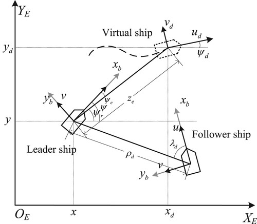
Control Objective: The objective of this note is to design a robust fuzzy dynamic surface formation control algorithm for USVs under uncertain dynamics and environmental disturbances such that: (1) All signals in the closed-loop system are semi-global uniformly ultimately bounded (SGUUB) stability; and (2) The leader can track the reference path generated by the virtual ship, and the follower can track the leader with the desired distance ${\rho }_d$ and desired angle ${\lambda }_d$ relative to the trajectory of leader; see Figure 1.

Figure 1. Schematic diagram of the leader-following framework.

2.2. Fuzzy logic system

There exists four parts for an FLS, i.e. the knowledge base, the fuzzifier, the fuzzy inference engine, and the defuzzifier. The knowledge base comprises a collection of fuzzy IF-THEN rules.

$R^l$: If $x_1$ is $F_1^l$ and $x_2$ is $F_2^l$ and … $x_n$ is $F_n^l$, then y is $G^l$. where $x=[x_1,\dots ,x_n{]}^{\mathrm{T}}$ and y are the input and output of the FLS, respectively. $F_i^l,i=1,2,\dots ,n$ and $G^l$ denote the fuzzy sets. ${\mu }_{F_i^l}\left(x_i\right)$ and ${\mu }_{G^l}\left(y\right)$ are fuzzy memberships functions of these fuzzy sets. The rule number is N. By resorting to singleton function, centre average defuzzification and product inference, the FLS can be expressed as Equation (2(2) $\begin{array}{r}y\left(x\right)=\frac{\sum _{i=1}^N{\overline{y}}_l\prod _{i=1}^n{\mu }_{F_i^l}\left(x_i\right)}{\sum _{i=1}^N\left[\prod _{i=1}^n{\mu }_{F_i^l}\right(x_i\left)\right]}\end{array}$(2) ). (2) $\begin{array}{r}y\left(x\right)=\frac{\sum _{i=1}^N{\overline{y}}_l\prod _{i=1}^n{\mu }_{F_i^l}\left(x_i\right)}{\sum _{i=1}^N\left[\prod _{i=1}^n{\mu }_{F_i^l}\right(x_i\left)\right]}\end{array}$(2) where ${\overline{y}}_l=\underset{y\in \mathbb{R}}{max}{\mu }_{G^l}\left(y\right)$. Let the fuzzy basis functions as Equation (3(3) $\begin{array}{r}{\phi }_l=\frac{\prod _{i=1}^n{\mu }_{F_i^l}\left(x_i\right)}{\sum _{i=1}^N\left(\prod _{i=1}^n{\mu }_{F_i^l}\right(x_i\left)\right)}\end{array}$(3) ). (3) $\begin{array}{r}{\phi }_l=\frac{\prod _{i=1}^n{\mu }_{F_i^l}\left(x_i\right)}{\sum _{i=1}^N\left(\prod _{i=1}^n{\mu }_{F_i^l}\right(x_i\left)\right)}\end{array}$(3) Denoting θ $=[{\overline{y}}_1,$ ${\overline{y}}_2,$ …, ${\overline{y}}_N{]}^{\mathrm{T}}$ $=[{\theta }_1,$ ${\theta }_2,$ …, ${\theta }_N{]}^{\mathrm{T}}$ and ${\phi }^{\mathrm{T}}\left(x\right)$ $=\left[{\phi }_1\right(x)$ $,{\phi }_2\left(x\right),$ $\dots ,{\phi }_N\left(x\right)]$. Then, the FLS (2(2) $\begin{array}{r}y\left(x\right)=\frac{\sum _{i=1}^N{\overline{y}}_l\prod _{i=1}^n{\mu }_{F_i^l}\left(x_i\right)}{\sum _{i=1}^N\left[\prod _{i=1}^n{\mu }_{F_i^l}\right(x_i\left)\right]}\end{array}$(2) ) can be rewritten as Equation (4(4) $\begin{array}{r}y\left(x\right)={\theta }^{\mathrm{T}}\phi \left(x\right)\end{array}$(4) ). (4) $\begin{array}{r}y\left(x\right)={\theta }^{\mathrm{T}}\phi \left(x\right)\end{array}$(4)

Lemma 2.1

Li et al., 2016

For any continuous function $f\left(x\right)$ defined in a compact set Ω, and for any random approximation error ε, $ϵ<{ϵ}_M$, there exists an FLS (4(4) $\begin{array}{r}y\left(x\right)={\theta }^{\mathrm{T}}\phi \left(x\right)\end{array}$(4) ) such that (5) $\begin{array}{r}\underset{x\in \mathrm{\Omega }}{sup}\left|f\right(x)-{\theta }^{\mathrm{T}}\phi (x\left)\right|\le ϵ\end{array}$(5)

3. Robust fuzzy dynamic surface formation controller design

In this section, one develops the robust fuzzy dynamic surface formation controller for USVs (1(1) $\begin{array}{r}\{\begin{array}{l}\dot{x}=u\cos \left(\psi \right)-v\sin \left(\psi \right)\\ \dot{y}=u\sin \left(\psi \right)+v\cos \left(\psi \right)\\ \dot{\psi }=r\\ \dot{u}=-f_u\left(\mathit{v}\right)+\frac{{\tau }_u}{m_u}+d_{wu}\\ \dot{v}=-f_v\left(\mathit{v}\right)+d_{wv}\\ \dot{r}=-f_r\left(\mathit{v}\right)+\frac{{\tau }_r}{m_r}+d_{wr}\end{array}\end{array}$(1) ) under Assumptions 2.1–2.2. To construct the desired formation configuration, the leader-following approach is adopted in Section 3.1, and a virtual ship is introduced to generate the smooth reference path. The control design procedure includes two steps for the kinematic and kinetic parts, which will be exhibited in Section 3.2. Finally, The corresponding stability analysis is demonstrated in Section 3.3.

3.1. Programming of the leader-following framework

In the leader-following framework, the leader ship and the follower ship act as two dominant roles. The schematic diagram of the leader-following formation system is displayed in Figure 1. The tracking signals of the leader is generated by the virtual ship, and the reference trajectory of the follower is generated by the trajectory of the leader. For this purpose, the leader-following formation control problem can be transformed into a two-layer tracking problem: First, drive the leader to track the reference path generated by the virtual ship. Second, let the follower ship to track the reference path of leader combined with the desired distance ${\rho }_d$ and the desired angle ${\lambda }_d$.

Part 1: To generate the reference path for the leader ship, a virtual ship, i.e. an ideal ship with no inertial and damping effects, is developed as Equation (6(6) $\begin{array}{r}\{\begin{array}{l}{\dot{x}}_d=u_d\cos \left({\psi }_d\right)\\ {\dot{y}}_d=u_d\sin \left({\psi }_d\right)\\ {\dot{\psi }}_d=r_d\end{array}\end{array}$(6) ). It is noted that the surge velocity $u_d$ is set by the user, and the turning angular velocity $r_d$ depends on the ship manoeuverability. Then, the generated desired position vector ${\mathit{\eta }}_d=[x_d,y_d,{\psi }_d{]}^{\mathrm{T}}$ can be provided to the leader for tracking. (6) $\begin{array}{r}\{\begin{array}{l}{\dot{x}}_d=u_d\cos \left({\psi }_d\right)\\ {\dot{y}}_d=u_d\sin \left({\psi }_d\right)\\ {\dot{\psi }}_d=r_d\end{array}\end{array}$(6) Part 2: By utilizing the real-time attitude information of the leader, the corresponding reference signals of follower ship can be derived as Equation (7(7) $\begin{array}{r}{\mathit{\eta }}_f={\mathit{\eta }}_d+\mathit{R}\left({\psi }_d\right)\mathit{l}\end{array}$(7) ) with the specific formation constraints, i.e.the desired distance ${\rho }_d$ and desired bearing angle ${\lambda }_d$. In Equation (7(7) $\begin{array}{r}{\mathit{\eta }}_f={\mathit{\eta }}_d+\mathit{R}\left({\psi }_d\right)\mathit{l}\end{array}$(7) ), ${\mathit{\eta }}_f$ denotes the desired reference signal vector of the followers and can be expressed as ${\mathit{\eta }}_f=[x_f,y_f,{\psi }_f{]}^{\mathrm{T}}$. $x_f$ and $y_f$ are the desired position information, and ${\psi }_d$ is the desired heading angle of follower ship. (7) $\begin{array}{r}{\mathit{\eta }}_f={\mathit{\eta }}_d+\mathit{R}\left({\psi }_d\right)\mathit{l}\end{array}$(7) with (8) $\begin{array}{rl}\mathit{R}\left({\psi }_d\right)& =\left[\begin{array}{ccc}\cos \left({\psi }_d\right)& -\sin \left({\psi }_d\right)& 0\\ \sin \left({\psi }_d\right)& \cos \left({\psi }_d\right)& 0\\ 0& 0& 1\end{array}\right],\\ \mathit{l}& =\left[\begin{array}{c}{\rho }_d\cos \left({\lambda }_d\right)\\ {\rho }_d\sin \left({\lambda }_d\right)\\ 0\end{array}\right]\end{array}$(8)

3.2. Control design

In this section, the robust fuzzy dynamic surface formation control algorithm is developed for USVs in the Backstepping framework. To avoid the repeated differentiation of the virtual control laws, an improved DSC technique is designed by introducing two second-order filters. Different from the traditional DSC methods, the proposed technique can eliminate the ‘explosion of complexity’ without the requirement of filter errors in the stability analysis. The corresponding design procedure can be divided into two steps: kinematics errors stabilization and kinetics errors stabilization.

Step 1: According to Figure 1, the kinematics errors, i.e. the position error and the heading error, can be expressed as Equation (9(9) $\begin{array}{r}\begin{array}{rl}{x}_e& =x_d-x,y_e=y_d-y\\ {\psi }_e& ={\psi }_r-\psi ,z_e=\sqrt{x_e^2+y_e^2}\end{array}\end{array}$(9) ). (9) $\begin{array}{r}\begin{array}{rl}{x}_e& =x_d-x,y_e=y_d-y\\ {\psi }_e& ={\psi }_r-\psi ,z_e=\sqrt{x_e^2+y_e^2}\end{array}\end{array}$(9) where ${\psi }_r$ denotes the azimuth angle between the virtual ship and the actual ship, which can be calculated as Equation (10(10) $\begin{array}{r}{\psi }_r=\{\begin{array}{l}{\displaystyle \frac{1}{2}}[1-\mathrm{s}\mathrm{g}\mathrm{n}\left(x_e\right)]\\ \mathrm{s}\mathrm{g}\mathrm{n}\left(y_e\right)\pi +\arctan \left({\displaystyle \frac{y_e}{x_e}}\right),& \mathrm{i}\mathrm{f}{x}_e\ne 0\\ +{\displaystyle \frac{\pi }{2}},& \mathrm{i}\mathrm{f}{x}_e=0\mathrm{a}\mathrm{n}\mathrm{d}{y}_e>0\\ -{\displaystyle \frac{\pi }{2}},& \mathrm{i}\mathrm{f}{x}_e=0\mathrm{a}\mathrm{n}\mathrm{d}{y}_e<0\\ {\psi }_d,& \mathrm{i}\mathrm{f}{x}_e=0\mathrm{a}\mathrm{n}\mathrm{d}{y}_e=0\end{array}\end{array}$(10) ). (10) $\begin{array}{r}{\psi }_r=\{\begin{array}{l}{\displaystyle \frac{1}{2}}[1-\mathrm{s}\mathrm{g}\mathrm{n}\left(x_e\right)]\\ \mathrm{s}\mathrm{g}\mathrm{n}\left(y_e\right)\pi +\arctan \left({\displaystyle \frac{y_e}{x_e}}\right),& \mathrm{i}\mathrm{f}{x}_e\ne 0\\ +{\displaystyle \frac{\pi }{2}},& \mathrm{i}\mathrm{f}{x}_e=0\mathrm{a}\mathrm{n}\mathrm{d}{y}_e>0\\ -{\displaystyle \frac{\pi }{2}},& \mathrm{i}\mathrm{f}{x}_e=0\mathrm{a}\mathrm{n}\mathrm{d}{y}_e<0\\ {\psi }_d,& \mathrm{i}\mathrm{f}{x}_e=0\mathrm{a}\mathrm{n}\mathrm{d}{y}_e=0\end{array}\end{array}$(10) By calculating the derivation of the kinematics errors (9(9) $\begin{array}{r}\begin{array}{rl}{x}_e& =x_d-x,y_e=y_d-y\\ {\psi }_e& ={\psi }_r-\psi ,z_e=\sqrt{x_e^2+y_e^2}\end{array}\end{array}$(9) ), one can obtain Equation (11(11) $\begin{array}{r}\begin{array}{rl}{\dot{z}}_e& ={\dot{x}}_d\cos \left({\psi }_r\right)+{\dot{y}}_d\sin \left({\psi }_r\right)-v\sin \left({\psi }_e\right)\\ & +2u{\sin }^2\left(0.5{\psi }_e\right)-u\\ {\dot{\psi }}_e& ={\dot{\psi }}_r-r\end{array}\end{array}$(11) ). (11) $\begin{array}{r}\begin{array}{rl}{\dot{z}}_e& ={\dot{x}}_d\cos \left({\psi }_r\right)+{\dot{y}}_d\sin \left({\psi }_r\right)-v\sin \left({\psi }_e\right)\\ & +2u{\sin }^2\left(0.5{\psi }_e\right)-u\\ {\dot{\psi }}_e& ={\dot{\psi }}_r-r\end{array}\end{array}$(11) To facilitate the design of the virtual controller, one define the kinetics errors as $u_e={\text{β}}_u-u$, $r_e={\text{β}}_r-r$. Thus, the derivation of the kinematics errors can be further expressed as Equation (12(12) $\begin{array}{r}\begin{array}{rl}{\dot{z}}_e& =\mathrm{\Pi }+u_e-({\text{β}}_u-{\alpha }_u)-{\alpha }_u\\ {\dot{\psi }}_e& ={\dot{\psi }}_r+r_e-({\text{β}}_r-{\alpha }_r)-{\alpha }_r\end{array}\end{array}$(12) ). (12) $\begin{array}{r}\begin{array}{rl}{\dot{z}}_e& =\mathrm{\Pi }+u_e-({\text{β}}_u-{\alpha }_u)-{\alpha }_u\\ {\dot{\psi }}_e& ={\dot{\psi }}_r+r_e-({\text{β}}_r-{\alpha }_r)-{\alpha }_r\end{array}\end{array}$(12) where ${\alpha }_i$ is the virtual control law, and ${\text{β}}_i$ is its filter version. i = u, r. $\mathrm{\Pi }={\dot{x}}_d\cos \left({\psi }_r\right)+{\dot{y}}_d\sin \left({\psi }_r\right)-v\sin \left({\psi }_e\right)+2u{\sin }^2\left(0.5{\psi }_e\right)$. Due to ${\dot{x}}_d$, ${\dot{y}}_d$, v and u are all bounded, it is obvious that Π is also bounded.

In the traditional adaptive Backstepping framework, the virtual control laws are required to be differentiated repeatedly to obtain their analytical derivatives. Thus, it may cause the problem of ‘explosion of complexity’, which can lead to the appearance of the undesired computational load. Fortunately, the DSC technique has been employed to eliminate this constraint, and no derived filtered errors are required to be stabilized in real-time. To be specific, let the virtual control laws pass through the second-order filters (13(13) $\begin{array}{r}\{\begin{array}{l}{\dot{\text{β}}}_i={\gamma }_i{\text{β}}_{i2}\\ {\dot{\text{β}}}_{i2}=-2{\xi }_i{\gamma }_i{\text{β}}_{i2}-{\gamma }_i({\text{β}}_i-{\alpha }_i)\end{array}\end{array}$(13) ). ${\text{β}}_i$ and ${\text{β}}_{2i}$ are the output signals. ${\gamma }_i>0$ is the natural frequency. ${\xi }_i\in (0,1]$ is the damping parameters. Once the virtual control law ${\alpha }_i$ satisfies the condition, the filtered error $({\text{β}}_i-{\alpha }_i)$ can be adjusted as a enough small constant to guarantee the convergence performance of the designed filters. (13) $\begin{array}{r}\{\begin{array}{l}{\dot{\text{β}}}_i={\gamma }_i{\text{β}}_{i2}\\ {\dot{\text{β}}}_{i2}=-2{\xi }_i{\gamma }_i{\text{β}}_{i2}-{\gamma }_i({\text{β}}_i-{\alpha }_i)\end{array}\end{array}$(13) Then, the compensating signals $q_{i1}$ and $q_{i2}$ can be developed as the following equation. (14) $\begin{array}{r}\begin{array}{r}\{\begin{array}{l}{\dot{q}}_{i1}=-k_{zi1}{q}_{i1}-({\text{β}}_i-{\alpha }_i)\\ {\dot{q}}_{i2}=-k_{zi2}{q}_{i2}\end{array}\end{array}\end{array}$(14) Considering the filtered errors compensation term, the new kinematic error can be defined as $z_e^{\star }=z_e-q_{u1}$, ${\psi }_e^{\star }={\psi }_e-q_{r1}$. Then, their derivative values can be obtained as Equation (15(15) $\begin{array}{r}\begin{array}{rl}{\dot{z}}_e^{\star }& =\mathrm{\Pi }+u_e-{\alpha }_u+k_{zu1}{q}_{u1}\\ {\dot{\psi }}_e^{\star }& ={\dot{\psi }}_r+r_e-{\alpha }_r+k_{zr1}{q}_{r1}\end{array}\end{array}$(15) ). (15) $\begin{array}{r}\begin{array}{rl}{\dot{z}}_e^{\star }& =\mathrm{\Pi }+u_e-{\alpha }_u+k_{zu1}{q}_{u1}\\ {\dot{\psi }}_e^{\star }& ={\dot{\psi }}_r+r_e-{\alpha }_r+k_{zr1}{q}_{r1}\end{array}\end{array}$(15) To stabilize the kinematic error, the virtual control laws can be derived as Equation (16(16) $\begin{array}{r}\begin{array}{rl}{\alpha }_u& =k_{zu1}{z}_e+\mathrm{\Pi }+q_{u2}\\ {\alpha }_r& =k_{zr1}{\psi }_e+{\dot{\psi }}_r+q_{r2}\end{array}\end{array}$(16) ). (16) $\begin{array}{r}\begin{array}{rl}{\alpha }_u& =k_{zu1}{z}_e+\mathrm{\Pi }+q_{u2}\\ {\alpha }_r& =k_{zr1}{\psi }_e+{\dot{\psi }}_r+q_{r2}\end{array}\end{array}$(16) Step 2: In this step, the final controller will be designed to stabilize the kinetics errors. For the purpose, the derivation of the tracking errors can be derived as Equation (17(17) $\begin{array}{r}\begin{array}{rl}{\dot{u}}_e& ={\dot{\text{β}}}_u-\dot{u}={\dot{\text{β}}}_u+f_u\left(\mathit{v}\right)-\frac{1}{m_u}{\tau }_u-d_{wu}\\ {\dot{r}}_e& ={\dot{\text{β}}}_r-\dot{r}={\dot{\text{β}}}_r+f_r\left(\mathit{v}\right)-\frac{1}{m_r}{\tau }_r-d_{wr}\end{array}\end{array}$(17) ). (17) $\begin{array}{r}\begin{array}{rl}{\dot{u}}_e& ={\dot{\text{β}}}_u-\dot{u}={\dot{\text{β}}}_u+f_u\left(\mathit{v}\right)-\frac{1}{m_u}{\tau }_u-d_{wu}\\ {\dot{r}}_e& ={\dot{\text{β}}}_r-\dot{r}={\dot{\text{β}}}_r+f_r\left(\mathit{v}\right)-\frac{1}{m_r}{\tau }_r-d_{wr}\end{array}\end{array}$(17) Combining the approximation theory, i.e. Lemma 2.1, the unknown system function can be addressed as Equation (18(18) $\begin{array}{rl}{f}_i\left(\mathit{v}\right)& ={\mathit{S}}_i\left(\mathit{v}\right){\mathit{A}}_i\mathit{v}+{ϵ}_i\\ & ={\mathit{S}}_i\left(\mathit{v}\right){\mathit{A}}_i{\text{β}}_v-{\mathit{S}}_i\left(\mathit{v}\right){\mathit{A}}_i{\mathit{v}}_e+{ϵ}_i\\ & ={\mathit{S}}_i\left(\mathit{v}\right){\mathit{A}}_i{\text{β}}_v-b_i\mathit{S}\left(\mathit{v}\right){\mathit{w}}_i+{ϵ}_i\end{array}$(18) ). (18) $\begin{array}{rl}{f}_i\left(\mathit{v}\right)& ={\mathit{S}}_i\left(\mathit{v}\right){\mathit{A}}_i\mathit{v}+{ϵ}_i\\ & ={\mathit{S}}_i\left(\mathit{v}\right){\mathit{A}}_i{\text{β}}_v-{\mathit{S}}_i\left(\mathit{v}\right){\mathit{A}}_i{\mathit{v}}_e+{ϵ}_i\\ & ={\mathit{S}}_i\left(\mathit{v}\right){\mathit{A}}_i{\text{β}}_v-b_i\mathit{S}\left(\mathit{v}\right){\mathit{w}}_i+{ϵ}_i\end{array}$(18) where ${\text{β}}_v=[{\text{β}}_u,v,{\text{β}}_r{]}^{\mathrm{T}}$,${\mathit{v}}_e=[u_e,0,r_e{]}^{\mathrm{T}}$. One defines $b_i=\Vert \mathit{A}\Vert$ and ${\mathit{A}}_i^m=\Vert {\mathit{A}}_i\Vert$, thus, ${\mathit{w}}_i={\mathit{A}}_i^m{\mathit{v}}_e$, $b_i{\mathit{w}}_i={\mathit{A}}_i{\mathit{v}}_e,i=u,r$. By incorporating the filtered compensating signals, the new tracking errors can be defined as $u_e^{\star }=u_e-q_{u2}$, $r_e^{\star }=r_e-q_{r2}$. From Equation (17(17) $\begin{array}{r}\begin{array}{rl}{\dot{u}}_e& ={\dot{\text{β}}}_u-\dot{u}={\dot{\text{β}}}_u+f_u\left(\mathit{v}\right)-\frac{1}{m_u}{\tau }_u-d_{wu}\\ {\dot{r}}_e& ={\dot{\text{β}}}_r-\dot{r}={\dot{\text{β}}}_r+f_r\left(\mathit{v}\right)-\frac{1}{m_r}{\tau }_r-d_{wr}\end{array}\end{array}$(17) ) and Equation (18(18) $\begin{array}{rl}{f}_i\left(\mathit{v}\right)& ={\mathit{S}}_i\left(\mathit{v}\right){\mathit{A}}_i\mathit{v}+{ϵ}_i\\ & ={\mathit{S}}_i\left(\mathit{v}\right){\mathit{A}}_i{\text{β}}_v-{\mathit{S}}_i\left(\mathit{v}\right){\mathit{A}}_i{\mathit{v}}_e+{ϵ}_i\\ & ={\mathit{S}}_i\left(\mathit{v}\right){\mathit{A}}_i{\text{β}}_v-b_i\mathit{S}\left(\mathit{v}\right){\mathit{w}}_i+{ϵ}_i\end{array}$(18) ), the derivation of the kinetic errors can be calculated as Equation (19(19) $\begin{array}{r}\begin{array}{rl}{\dot{u}}_e^{\star }& ={\dot{u}}_e-{\dot{q}}_{u2}={\dot{\text{β}}}_u+{\mathit{S}}_u\left(\mathit{v}\right){\mathit{A}}_u{\text{β}}_v\\ & -b_u{\mathit{S}}_u\left(\mathit{v}\right){\mathit{w}}_u+{ϵ}_u-\frac{1}{m_u}{\tau }_u-d_{wu}\\ {\dot{r}}_e^{\star }& ={\dot{r}}_e-{\dot{q}}_{r2}={\dot{\text{β}}}_r+{\mathit{S}}_r\left(\mathit{v}\right){\mathit{A}}_r{\text{β}}_v\\ & -b_r{\mathit{S}}_r\left(\mathit{v}\right){\mathit{w}}_r+{ϵ}_r-\frac{1}{m_r}{\tau }_r-d_{wr}\end{array}\end{array}$(19) ). (19) $\begin{array}{r}\begin{array}{rl}{\dot{u}}_e^{\star }& ={\dot{u}}_e-{\dot{q}}_{u2}={\dot{\text{β}}}_u+{\mathit{S}}_u\left(\mathit{v}\right){\mathit{A}}_u{\text{β}}_v\\ & -b_u{\mathit{S}}_u\left(\mathit{v}\right){\mathit{w}}_u+{ϵ}_u-\frac{1}{m_u}{\tau }_u-d_{wu}\\ {\dot{r}}_e^{\star }& ={\dot{r}}_e-{\dot{q}}_{r2}={\dot{\text{β}}}_r+{\mathit{S}}_r\left(\mathit{v}\right){\mathit{A}}_r{\text{β}}_v\\ & -b_r{\mathit{S}}_r\left(\mathit{v}\right){\mathit{w}}_r+{ϵ}_r-\frac{1}{m_r}{\tau }_r-d_{wr}\end{array}\end{array}$(19) Therefore, the final controller can be derived as Equation (20(20) $\begin{array}{rl}& \begin{array}{rl}{\tau }_u& =m_u[k_{zu2}{u}_e+{\dot{\text{β}}}_u+{\hat{\lambda }}_u{\mathrm{\Phi }}_u(\cdot \left)u_e^{\star }\right]\\ {\tau }_r& =m_r[k_{zr2}{r}_e+{\dot{\text{β}}}_r+{\hat{\lambda }}_r{\mathrm{\Phi }}_r(\cdot \left)r_e^{\star }\right]\end{array}\end{array}$(20) ), and the adaptive learning parameters can be calculated as Equation (21(21) $\begin{array}{rl}& \begin{array}{rl}& {\dot{\hat{\lambda }}}_u={\mathrm{\Gamma }}_{{\lambda }_u}\left[{\mathrm{\Phi }}_u\right(\cdot ){u_e^{\star }}^2-{\sigma }_{{\lambda }_u}({\hat{\lambda }}_u-{\hat{\lambda }}_u(0\left)\right)]\\ & {\dot{\hat{\lambda }}}_r={\mathrm{\Gamma }}_{{\lambda }_r}\left[{\mathrm{\Phi }}_r\right(\cdot ){r_e^{\star }}^2-{\sigma }_{{\lambda }_r}({\hat{\lambda }}_r-{\hat{\lambda }}_r(0\left)\right)]\end{array}\end{array}$(21) ). (20) $\begin{array}{rl}& \begin{array}{rl}{\tau }_u& =m_u[k_{zu2}{u}_e+{\dot{\text{β}}}_u+{\hat{\lambda }}_u{\mathrm{\Phi }}_u(\cdot \left)u_e^{\star }\right]\\ {\tau }_r& =m_r[k_{zr2}{r}_e+{\dot{\text{β}}}_r+{\hat{\lambda }}_r{\mathrm{\Phi }}_r(\cdot \left)r_e^{\star }\right]\end{array}\end{array}$(20) (21) $\begin{array}{rl}& \begin{array}{rl}& {\dot{\hat{\lambda }}}_u={\mathrm{\Gamma }}_{{\lambda }_u}\left[{\mathrm{\Phi }}_u\right(\cdot ){u_e^{\star }}^2-{\sigma }_{{\lambda }_u}({\hat{\lambda }}_u-{\hat{\lambda }}_u(0\left)\right)]\\ & {\dot{\hat{\lambda }}}_r={\mathrm{\Gamma }}_{{\lambda }_r}\left[{\mathrm{\Phi }}_r\right(\cdot ){r_e^{\star }}^2-{\sigma }_{{\lambda }_r}({\hat{\lambda }}_r-{\hat{\lambda }}_r(0\left)\right)]\end{array}\end{array}$(21) where ${\mathrm{\Phi }}_i(\cdot )$ is the robust damping term, which will be designed in Section 3.3. $k_{zu2}$, $k_{zr2}$, ${\mathrm{\Gamma }}_{{\lambda }_u}$, ${\mathrm{\Gamma }}_{{\lambda }_r}$, ${\sigma }_{{\lambda }_u}$, ${\sigma }_{{\lambda }_r}$ are the positive parameters. ${\hat{\lambda }}_i\left(0\right)$ denotes the initial value of ${\hat{\lambda }}_i$. i = u, r.

3.3. Stability analysis

Based on the above discussion, one has the main results as follows:

Theorem 3.1

Consider the mathematical model of underactuated ships (1(1) $\begin{array}{r}\{\begin{array}{l}\dot{x}=u\cos \left(\psi \right)-v\sin \left(\psi \right)\\ \dot{y}=u\sin \left(\psi \right)+v\cos \left(\psi \right)\\ \dot{\psi }=r\\ \dot{u}=-f_u\left(\mathit{v}\right)+\frac{{\tau }_u}{m_u}+d_{wu}\\ \dot{v}=-f_v\left(\mathit{v}\right)+d_{wv}\\ \dot{r}=-f_r\left(\mathit{v}\right)+\frac{{\tau }_r}{m_r}+d_{wr}\end{array}\end{array}$(1) ) satisfying Assumptions 2.1–2.2, For all initial conditions satisfying ${z_e^{\star }}^2\left(0\right)+{{\psi }_e^{\star }}^2\left(0\right)+{u_e^{\star }}^2\left(0\right)+{r_e^{\star }}^2\left(0\right)+{\tilde{\lambda }}_u^2\left(0\right)+{\tilde{\lambda }}_r^2\left(0\right)\le 2\mathrm{\Delta }$, with any $\mathrm{\Delta }>0$, one can adjust the control parameters $k_{zu1}$, $k_{zr1}$, $k_{zu2}$, $k_{zr2}$, ${\mathrm{\Gamma }}_{{\lambda }_u}$, ${\mathrm{\Gamma }}_{{\lambda }_r}$, ${\sigma }_{{\lambda }_u}$, ${\sigma }_{{\lambda }_r}$ appropriately, satisfying that all the signal variables and tracking errors of the closed-loop control system are semi-global uniformly ultimately bounded (SGUUB).

Proof.

First, one selects the following Lyapunov candidate function as Equation (22(22) $\begin{array}{r}V=\frac{1}{2}{z_e^{\star }}^2+\frac{1}{2}{{\psi }_e^{\star }}^2+\frac{1}{2}{u_e^{\star }}^2+\frac{1}{2}{r_e^{\star }}^2+\frac{1}{2{\mathrm{\Gamma }}_{{\lambda }_u}}{\tilde{\lambda }}_u^2+\frac{1}{2{\mathrm{\Gamma }}_{{\lambda }_r}}{\tilde{\lambda }}_r^2\end{array}$(22) ). (22) $\begin{array}{r}V=\frac{1}{2}{z_e^{\star }}^2+\frac{1}{2}{{\psi }_e^{\star }}^2+\frac{1}{2}{u_e^{\star }}^2+\frac{1}{2}{r_e^{\star }}^2+\frac{1}{2{\mathrm{\Gamma }}_{{\lambda }_u}}{\tilde{\lambda }}_u^2+\frac{1}{2{\mathrm{\Gamma }}_{{\lambda }_r}}{\tilde{\lambda }}_r^2\end{array}$(22) By differentiating the Lyapunov function, tEquation (23(23) $\begin{array}{rl}\dot{V}& =z_e^{\star }{\dot{z_e}}^{\star }+{\psi }_e^{\star }{\dot{{\psi }_e}}^{\star }+u_e^{\star }{\dot{u_e}}^{\star }+r_e^{\star }{\dot{r_e}}^{\star }+{\mathrm{\Gamma }}_{{\lambda }_u}^{-1}{\tilde{\lambda }}_u^2{\dot{\tilde{\lambda }}}_u^2\\ & +{\mathrm{\Gamma }}_{{\lambda }_r}^{-1}{\tilde{\lambda }}_r^2{\dot{\tilde{\lambda }}}_r^2\end{array}$(23) ) can be obtained. (23) $\begin{array}{rl}\dot{V}& =z_e^{\star }{\dot{z_e}}^{\star }+{\psi }_e^{\star }{\dot{{\psi }_e}}^{\star }+u_e^{\star }{\dot{u_e}}^{\star }+r_e^{\star }{\dot{r_e}}^{\star }+{\mathrm{\Gamma }}_{{\lambda }_u}^{-1}{\tilde{\lambda }}_u^2{\dot{\tilde{\lambda }}}_u^2\\ & +{\mathrm{\Gamma }}_{{\lambda }_r}^{-1}{\tilde{\lambda }}_r^2{\dot{\tilde{\lambda }}}_r^2\end{array}$(23) From Equations (15(15) $\begin{array}{r}\begin{array}{rl}{\dot{z}}_e^{\star }& =\mathrm{\Pi }+u_e-{\alpha }_u+k_{zu1}{q}_{u1}\\ {\dot{\psi }}_e^{\star }& ={\dot{\psi }}_r+r_e-{\alpha }_r+k_{zr1}{q}_{r1}\end{array}\end{array}$(15) ), (16(16) $\begin{array}{r}\begin{array}{rl}{\alpha }_u& =k_{zu1}{z}_e+\mathrm{\Pi }+q_{u2}\\ {\alpha }_r& =k_{zr1}{\psi }_e+{\dot{\psi }}_r+q_{r2}\end{array}\end{array}$(16) ) and (19(19) $\begin{array}{r}\begin{array}{rl}{\dot{u}}_e^{\star }& ={\dot{u}}_e-{\dot{q}}_{u2}={\dot{\text{β}}}_u+{\mathit{S}}_u\left(\mathit{v}\right){\mathit{A}}_u{\text{β}}_v\\ & -b_u{\mathit{S}}_u\left(\mathit{v}\right){\mathit{w}}_u+{ϵ}_u-\frac{1}{m_u}{\tau }_u-d_{wu}\\ {\dot{r}}_e^{\star }& ={\dot{r}}_e-{\dot{q}}_{r2}={\dot{\text{β}}}_r+{\mathit{S}}_r\left(\mathit{v}\right){\mathit{A}}_r{\text{β}}_v\\ & -b_r{\mathit{S}}_r\left(\mathit{v}\right){\mathit{w}}_r+{ϵ}_r-\frac{1}{m_r}{\tau }_r-d_{wr}\end{array}\end{array}$(19) ), one can obtain the following inequality. (24) $\begin{array}{rl}\dot{V}& =-k_{zu1}{z_e^{\star }}^2+z_e^{\star }{u}_e^{\star }-k_{zr1}{{\psi }_e^{\star }}^2+{\psi }_e^{\star }{r}_e^{\star }\\ & +{\mathrm{\Gamma }}_{{\lambda }_u}^{-1}{\tilde{\lambda }}_u^2{\dot{\tilde{\lambda }}}_u^2+{\mathrm{\Gamma }}_{{\lambda }_r}^{-1}{\tilde{\lambda }}_r^2{\dot{\tilde{\lambda }}}_r^2\\ & +u_e^{\star }({\dot{\text{β}}}_u+{\mathit{S}}_u(\mathit{v}){\mathit{A}}_u{\text{β}}_v-b_u{\mathit{S}}_u(\mathit{v}){\mathit{w}}_u\\ & +{ϵ}_u-\frac{1}{m_u}{\tau }_u-d_{wu})\\ & +r_e^{\star }({\dot{\text{β}}}_r+{\mathit{S}}_r(\mathit{v}){\mathit{A}}_r{\text{β}}_v-b_r{\mathit{S}}_r(\mathit{v}){\mathit{w}}_r\\ & +{ϵ}_r-\frac{1}{m_r}{\tau }_r-d_{wr})\end{array}$(24) To facilitate the following analysis, Equation (25(25) $\begin{array}{rl}{\mathrm{\Xi }}_i& ={\mathit{S}}_i\left(\mathit{v}\right){\mathit{A}}_i{\text{β}}_v+{ϵ}_i-d_{wi}\\ & \le {\mathit{S}}_i\left(\mathit{v}\right){\mathit{A}}_i{\text{β}}_v+{\overline{ϵ}}_i+{\overline{d}}_{wi}\\ & \le {\vartheta }_i{\phi }_i\left(\mathit{v}\right)\end{array}$(25) ) is provided. Benefiting from the MLP technique, the system uncertain function and the unknown time-varying parameterized disturbance can be compressed transversely and the real-time updating of the fuzzy weight matrix can be avoided, which can overcome the problem of ‘curse of dimensionality’. (25) $\begin{array}{rl}{\mathrm{\Xi }}_i& ={\mathit{S}}_i\left(\mathit{v}\right){\mathit{A}}_i{\text{β}}_v+{ϵ}_i-d_{wi}\\ & \le {\mathit{S}}_i\left(\mathit{v}\right){\mathit{A}}_i{\text{β}}_v+{\overline{ϵ}}_i+{\overline{d}}_{wi}\\ & \le {\vartheta }_i{\phi }_i\left(\mathit{v}\right)\end{array}$(25) where ${\vartheta }_i=max\{\Vert \mathit{A}\Vert ,{\overline{ϵ}}_i+{\overline{d}}_{wi}\}$, ${\phi }_i\left(\mathit{v}\right)=1+\Vert {\mathit{S}}_i\left(\mathit{v}\right)\Vert \Vert {\text{β}}_v\Vert ,i=u,r$. (26) $\begin{array}{rl}-b_i{\mathit{S}}_i\left(\mathit{v}\right){\mathit{w}}_i{i}_e^{\star }& \le \frac{b_i^2{\mathit{S}}_i^{\mathrm{T}}\left(\mathit{v}\right){\mathit{S}}_i\left(\mathit{v}\right){i_e^{\star }}^2}{4{\gamma }_{i1}^2}+{\gamma }_{i1}^2{\mathit{w}}_i^{\mathrm{T}}{\mathit{w}}_i\end{array}$(26) (27) $\begin{array}{rl}{\vartheta }_i{\phi }_i\left(\mathit{v}\right)i_e^{\star }& \le \frac{{\vartheta }_i^2{\phi }_i(\mathit{v}{)}^2{i_e^{\star }}^2}{4{\gamma }_{i2}^2}+{\gamma }_{i2}^2\end{array}$(27) Noting that the definition of ${\mathit{w}}_i$, one can obtain (28) $\begin{array}{rl}{\mathit{w}}_i& ={\mathit{A}}_i^m{i}_e=\frac{{\mathit{A}}_i}{\parallel {\mathit{A}}_i\parallel }{i}_e=\frac{1}{\Vert {\mathit{A}}_i\Vert }\left[\begin{array}{c}{w}_{i1}{i}_e\\ w_{i2}{i}_e\\ ⋮\\ w_{il}{i}_e\end{array}\right]\end{array}$(28) (29) $\begin{array}{rl}{\mathit{w}}_i^{\mathrm{T}}{\mathit{w}}_i& =\frac{1}{\Vert {\mathit{A}}_i\Vert }(w_{i1}^2+w_{i2}^2+\cdots +w_{il}^2)i_e^2=i_e^2\end{array}$(29) Then, the terms $b_i^2{\mathit{S}}_i^{\mathrm{T}}\left(\mathit{v}\right){\mathit{S}}_i\left(\mathit{v}\right){i_e^{\star }}^2/\left(4{\gamma }_{i1}^2\right)$ and ${\vartheta }_i^2{\phi }_i(\mathit{v}{)}^2{i_e^{\star }}^2/\left(4{\gamma }_{i2}^2\right)$ can be further compressed as Equation (30(30) $\begin{array}{r}\frac{b_i^2{\mathit{S}}_i^{\mathrm{T}}\left(\mathit{v}\right){\mathit{S}}_i\left(\mathit{v}\right){i_e^{\star }}^2}{4{\gamma }_{i1}^2}+\frac{{\vartheta }_i^2{\phi }_i(\mathit{v}{)}^2{i_e^{\star }}^2}{4{\gamma }_{i2}^2}\le {\lambda }_i{\mathrm{\Phi }}_i(\cdot ){i_e^{\star }}^2\end{array}$(30) ). (30) $\begin{array}{r}\frac{b_i^2{\mathit{S}}_i^{\mathrm{T}}\left(\mathit{v}\right){\mathit{S}}_i\left(\mathit{v}\right){i_e^{\star }}^2}{4{\gamma }_{i1}^2}+\frac{{\vartheta }_i^2{\phi }_i(\mathit{v}{)}^2{i_e^{\star }}^2}{4{\gamma }_{i2}^2}\le {\lambda }_i{\mathrm{\Phi }}_i(\cdot ){i_e^{\star }}^2\end{array}$(30) where $\mathrm{\Phi }(\cdot )=\frac{{\mathit{S}}_i^{\mathrm{T}}\left(\mathit{v}\right){\mathit{S}}_i\left(\mathit{v}\right)}{4{\gamma }_{i1}^2}+\frac{{\phi }_i(\mathit{v}{)}^2}{4{\gamma }_{i2}^2}$, ${\lambda }_i=max\{b_i^2,{\vartheta }_i^2\}$. By submitting Equations (25(25) $\begin{array}{rl}{\mathrm{\Xi }}_i& ={\mathit{S}}_i\left(\mathit{v}\right){\mathit{A}}_i{\text{β}}_v+{ϵ}_i-d_{wi}\\ & \le {\mathit{S}}_i\left(\mathit{v}\right){\mathit{A}}_i{\text{β}}_v+{\overline{ϵ}}_i+{\overline{d}}_{wi}\\ & \le {\vartheta }_i{\phi }_i\left(\mathit{v}\right)\end{array}$(25) )–(30(30) $\begin{array}{r}\frac{b_i^2{\mathit{S}}_i^{\mathrm{T}}\left(\mathit{v}\right){\mathit{S}}_i\left(\mathit{v}\right){i_e^{\star }}^2}{4{\gamma }_{i1}^2}+\frac{{\vartheta }_i^2{\phi }_i(\mathit{v}{)}^2{i_e^{\star }}^2}{4{\gamma }_{i2}^2}\le {\lambda }_i{\mathrm{\Phi }}_i(\cdot ){i_e^{\star }}^2\end{array}$(30) ) into Equation (24(24) $\begin{array}{rl}\dot{V}& =-k_{zu1}{z_e^{\star }}^2+z_e^{\star }{u}_e^{\star }-k_{zr1}{{\psi }_e^{\star }}^2+{\psi }_e^{\star }{r}_e^{\star }\\ & +{\mathrm{\Gamma }}_{{\lambda }_u}^{-1}{\tilde{\lambda }}_u^2{\dot{\tilde{\lambda }}}_u^2+{\mathrm{\Gamma }}_{{\lambda }_r}^{-1}{\tilde{\lambda }}_r^2{\dot{\tilde{\lambda }}}_r^2\\ & +u_e^{\star }({\dot{\text{β}}}_u+{\mathit{S}}_u(\mathit{v}){\mathit{A}}_u{\text{β}}_v-b_u{\mathit{S}}_u(\mathit{v}){\mathit{w}}_u\\ & +{ϵ}_u-\frac{1}{m_u}{\tau }_u-d_{wu})\\ & +r_e^{\star }({\dot{\text{β}}}_r+{\mathit{S}}_r(\mathit{v}){\mathit{A}}_r{\text{β}}_v-b_r{\mathit{S}}_r(\mathit{v}){\mathit{w}}_r\\ & +{ϵ}_r-\frac{1}{m_r}{\tau }_r-d_{wr})\end{array}$(24) ), one can obtain the following inequality. (31) $\begin{array}{rl}\dot{V}& \le -(k_{zu1}-\frac{1}{4}){z_e^{\star }}^2-(k_{zr1}-\frac{1}{4}){{\psi }_e^{\star }}^2\\ & -(k_{zu2}-1){u_e^{\star }}^2-(k_{zr2}-1){r_e^{\star }}^2\\ & +{\gamma }_{u1}^2{u}_e^2+{\gamma }_{r1}^2{r}_e^2+{\gamma }_{u2}^2+{\gamma }_{r2}^2-\frac{{\sigma }_{{\lambda }_u}}{2}{\tilde{\lambda }}_u^2-\frac{{\sigma }_{{\lambda }_r}}{2}{\tilde{\lambda }}_r^2\\ & +\frac{{\sigma }_{{\lambda }_u}}{2}{({\lambda }_u-{\hat{\lambda }}_u(0\left)\right)}^2\\ & +\frac{{\sigma }_{{\lambda }_r}}{2}{({\lambda }_r-{\hat{\lambda }}_r(0\left)\right)}^2\end{array}$(31) Let $\mu =min\{k_{zu1}-1/4$,$k_{zr1}-1/4,k_{zu2}-1,k_{zr2}-1$, $-{\gamma }_{u1}^2$, $-{\gamma }_{r1}^2$, ${\mathrm{\Gamma }}_{{\lambda }_u}{\sigma }_{{\lambda }_u}/2,{\mathrm{\Gamma }}_{{\lambda }_r}{\sigma }_{{\lambda }_r}/2\}$, Equation (32(32) $\begin{array}{r}\dot{V}\le -2\mu V+\mathrm{\Delta }\end{array}$(32) ) can be further derived. (32) $\begin{array}{r}\dot{V}\le -2\mu V+\mathrm{\Delta }\end{array}$(32) where $\mathrm{\Delta }={\gamma }_{u2}^2+{\gamma }_{r2}^2+{\sigma }_{{\lambda }_u}/2({\lambda }_u-{\hat{\lambda }}_u(0){)}^2+{\sigma }_{{\lambda }_r}/2({\lambda }_r-{\hat{\lambda }}_r\left(0\right){)}^2$.

Integrate both sides of Equation (32(32) $\begin{array}{r}\dot{V}\le -2\mu V+\mathrm{\Delta }\end{array}$(32) ), the trajectory of V can be bounded by (33) $\begin{array}{r}V\left(t\right)\le \frac{\mathrm{\Delta }}{2\mu }+\left(V\right(0)-\frac{\mathrm{\Delta }}{2\mu })\exp (-2\mu t)\end{array}$(33) Obviously, one can obtain $\underset{t\to \mathrm{\infty }}{lim}V\left(t\right)=\mathrm{\Delta }/\left(2\mu \right)$. This means that all signals of the closed-loop control system are SGUUB stability, and the measurement errors are small enough which could be converge to zero by adjusting the designed parameters appropriately. The proof is finished.

The time-varying parameterized disturbances are highly nonlinear and have both low-frequency and high-frequency effects to the ship's motion. To enhance the robust performance of the proposed algorithm, the LFG technique is used and Corollary 3.1 is exhibited directly.

Corollary 3.1

Under Assumptions 2.1 and 2.2, one considers the ship dynamics (1(1) $\begin{array}{r}\{\begin{array}{l}\dot{x}=u\cos \left(\psi \right)-v\sin \left(\psi \right)\\ \dot{y}=u\sin \left(\psi \right)+v\cos \left(\psi \right)\\ \dot{\psi }=r\\ \dot{u}=-f_u\left(\mathit{v}\right)+\frac{{\tau }_u}{m_u}+d_{wu}\\ \dot{v}=-f_v\left(\mathit{v}\right)+d_{wv}\\ \dot{r}=-f_r\left(\mathit{v}\right)+\frac{{\tau }_r}{m_r}+d_{wr}\end{array}\end{array}$(1) ) and (2(2) $\begin{array}{r}y\left(x\right)=\frac{\sum _{i=1}^N{\overline{y}}_l\prod _{i=1}^n{\mu }_{F_i^l}\left(x_i\right)}{\sum _{i=1}^N\left[\prod _{i=1}^n{\mu }_{F_i^l}\right(x_i\left)\right]}\end{array}$(2) ) with initial conditions such that ${z_e^{\star }}^2\left(0\right)+{{\psi }_e^{\star }}^2\left(0\right)+{u_e^{\star }}^2\left(0\right)+{r_e^{\star }}^2\left(0\right)+{\tilde{\lambda }}_u^2\left(0\right)+{\tilde{\lambda }}_r^2\left(0\right)+{\tilde{\lambda }}_{uf}^2\left(0\right)+{\tilde{\lambda }}_{rf}^2\left(0\right)\le 2\mathrm{\Delta }$, with any $\mathrm{\Delta }>0$. The control efforts (20(20) $\begin{array}{rl}& \begin{array}{rl}{\tau }_u& =m_u[k_{zu2}{u}_e+{\dot{\text{β}}}_u+{\hat{\lambda }}_u{\mathrm{\Phi }}_u(\cdot \left)u_e^{\star }\right]\\ {\tau }_r& =m_r[k_{zr2}{r}_e+{\dot{\text{β}}}_r+{\hat{\lambda }}_r{\mathrm{\Phi }}_r(\cdot \left)r_e^{\star }\right]\end{array}\end{array}$(20) ) and the low-frequency gain-learning law (34(34) $\begin{array}{r}\{\begin{array}{l}{\dot{\hat{\lambda }}}_u={\mathrm{\Gamma }}_{{\lambda }_u}\left[{\mathrm{\Phi }}_u\right(\cdot ){u_e^{\star }}^2-{\sigma }_{{\lambda }_u}({\hat{\lambda }}_u-{\hat{\lambda }}_{uf})]{\dot{\hat{\lambda }}}_{uf}\\ ={\mathrm{\Gamma }}_{{\lambda }_{uf}}[{\hat{\lambda }}_u-{\hat{\lambda }}_{uf}]\\ {\dot{\hat{\lambda }}}_r={\mathrm{\Gamma }}_{{\lambda }_r}\left[{\mathrm{\Phi }}_r\right(\cdot ){r_e^{\star }}^2-{\sigma }_{{\lambda }_r}({\hat{\lambda }}_r-{\hat{\lambda }}_{rf})]{\dot{\hat{\lambda }}}_{rf}\\ ={\mathrm{\Gamma }}_{{\lambda }_{rf}}[{\hat{\lambda }}_r-{\hat{\lambda }}_{rf}]\end{array}\end{array}$(34) ) can guarantee that the solution of the closed-loop control system is SGUUB: (34) $\begin{array}{r}\{\begin{array}{l}{\dot{\hat{\lambda }}}_u={\mathrm{\Gamma }}_{{\lambda }_u}\left[{\mathrm{\Phi }}_u\right(\cdot ){u_e^{\star }}^2-{\sigma }_{{\lambda }_u}({\hat{\lambda }}_u-{\hat{\lambda }}_{uf})]{\dot{\hat{\lambda }}}_{uf}\\ ={\mathrm{\Gamma }}_{{\lambda }_{uf}}[{\hat{\lambda }}_u-{\hat{\lambda }}_{uf}]\\ {\dot{\hat{\lambda }}}_r={\mathrm{\Gamma }}_{{\lambda }_r}\left[{\mathrm{\Phi }}_r\right(\cdot ){r_e^{\star }}^2-{\sigma }_{{\lambda }_r}({\hat{\lambda }}_r-{\hat{\lambda }}_{rf})]{\dot{\hat{\lambda }}}_{rf}\\ ={\mathrm{\Gamma }}_{{\lambda }_{rf}}[{\hat{\lambda }}_r-{\hat{\lambda }}_{rf}]\end{array}\end{array}$(34) where ${\hat{\lambda }}_{uf}$ and ${\hat{\lambda }}_{rf}$ are the filtered estimations of ${\lambda }_u$ and ${\lambda }_r$, and ${\tilde{\lambda }}_{uf}={\hat{\lambda }}_{uf}-{\lambda }_{uf}$, ${\tilde{\lambda }}_{rf}={\hat{\lambda }}_{rf}-{\lambda }_{rf}$.

Proof.

Corollary 3.1 is the application of Theorem 1 to the proposed control algorithm. For the low-frequency adaptive law (34(34) $\begin{array}{r}\{\begin{array}{l}{\dot{\hat{\lambda }}}_u={\mathrm{\Gamma }}_{{\lambda }_u}\left[{\mathrm{\Phi }}_u\right(\cdot ){u_e^{\star }}^2-{\sigma }_{{\lambda }_u}({\hat{\lambda }}_u-{\hat{\lambda }}_{uf})]{\dot{\hat{\lambda }}}_{uf}\\ ={\mathrm{\Gamma }}_{{\lambda }_{uf}}[{\hat{\lambda }}_u-{\hat{\lambda }}_{uf}]\\ {\dot{\hat{\lambda }}}_r={\mathrm{\Gamma }}_{{\lambda }_r}\left[{\mathrm{\Phi }}_r\right(\cdot ){r_e^{\star }}^2-{\sigma }_{{\lambda }_r}({\hat{\lambda }}_r-{\hat{\lambda }}_{rf})]{\dot{\hat{\lambda }}}_{rf}\\ ={\mathrm{\Gamma }}_{{\lambda }_{rf}}[{\hat{\lambda }}_r-{\hat{\lambda }}_{rf}]\end{array}\end{array}$(34) ), the partial Lyapunov candidate can be established as Equation (35(35) $\begin{array}{r}{V}_{\lambda }=\frac{1}{2{\mathrm{\Gamma }}_{{\lambda }_u}}{\tilde{\lambda }}_u^2+\frac{{\sigma }_{{\lambda }_u}}{2{\mathrm{\Gamma }}_{{\lambda }_{uf}}}{\tilde{\lambda }}_{uf}^2+\frac{1}{2{\mathrm{\Gamma }}_{{\lambda }_r}}{\tilde{\lambda }}_r^2+\frac{{\sigma }_{{\lambda }_r}}{2{\mathrm{\Gamma }}_{{\lambda }_{rf}}}{\tilde{\lambda }}_{rf}^2\end{array}$(35) ). (35) $\begin{array}{r}{V}_{\lambda }=\frac{1}{2{\mathrm{\Gamma }}_{{\lambda }_u}}{\tilde{\lambda }}_u^2+\frac{{\sigma }_{{\lambda }_u}}{2{\mathrm{\Gamma }}_{{\lambda }_{uf}}}{\tilde{\lambda }}_{uf}^2+\frac{1}{2{\mathrm{\Gamma }}_{{\lambda }_r}}{\tilde{\lambda }}_r^2+\frac{{\sigma }_{{\lambda }_r}}{2{\mathrm{\Gamma }}_{{\lambda }_{rf}}}{\tilde{\lambda }}_{rf}^2\end{array}$(35) The relevant derivative of the Lyapunov function can be deduced as Equation (36(36) $\begin{array}{rl}{\dot{V}}_{\lambda }& ={\tilde{\lambda }}_u{\mathrm{\Phi }}_u(\cdot ){u_e^{\star }}^2+{\tilde{\lambda }}_r{\mathrm{\Phi }}_r(\cdot ){r_e^{\star }}^2\\ & -\sum _{i=u,r}{\sigma }_{{\lambda }_i}({\tilde{\lambda }}_i^2-2{\tilde{\lambda }}_i{\tilde{\lambda }}_{if}+{\tilde{\lambda }}_{if}^2)\\ & \le {\tilde{\lambda }}_u{\mathrm{\Phi }}_u(\cdot ){u_e^{\star }}^2+{\tilde{\lambda }}_r{\mathrm{\Phi }}_r(\cdot ){r_e^{\star }}^2\end{array}$(36) ). (36) $\begin{array}{rl}{\dot{V}}_{\lambda }& ={\tilde{\lambda }}_u{\mathrm{\Phi }}_u(\cdot ){u_e^{\star }}^2+{\tilde{\lambda }}_r{\mathrm{\Phi }}_r(\cdot ){r_e^{\star }}^2\\ & -\sum _{i=u,r}{\sigma }_{{\lambda }_i}({\tilde{\lambda }}_i^2-2{\tilde{\lambda }}_i{\tilde{\lambda }}_{if}+{\tilde{\lambda }}_{if}^2)\\ & \le {\tilde{\lambda }}_u{\mathrm{\Phi }}_u(\cdot ){u_e^{\star }}^2+{\tilde{\lambda }}_r{\mathrm{\Phi }}_r(\cdot ){r_e^{\star }}^2\end{array}$(36) In Equation (36(36) $\begin{array}{rl}{\dot{V}}_{\lambda }& ={\tilde{\lambda }}_u{\mathrm{\Phi }}_u(\cdot ){u_e^{\star }}^2+{\tilde{\lambda }}_r{\mathrm{\Phi }}_r(\cdot ){r_e^{\star }}^2\\ & -\sum _{i=u,r}{\sigma }_{{\lambda }_i}({\tilde{\lambda }}_i^2-2{\tilde{\lambda }}_i{\tilde{\lambda }}_{if}+{\tilde{\lambda }}_{if}^2)\\ & \le {\tilde{\lambda }}_u{\mathrm{\Phi }}_u(\cdot ){u_e^{\star }}^2+{\tilde{\lambda }}_r{\mathrm{\Phi }}_r(\cdot ){r_e^{\star }}^2\end{array}$(36) ), the remainder term $\left({\tilde{\lambda }}_u{\mathrm{\Phi }}_u\right(\cdot ){u_e^{\star }}^2+{\tilde{\lambda }}_r{\mathrm{\Phi }}_r(\cdot \left){r_e^{\star }}^2\right)$ can be cancelled by the control effort (20(20) $\begin{array}{rl}& \begin{array}{rl}{\tau }_u& =m_u[k_{zu2}{u}_e+{\dot{\text{β}}}_u+{\hat{\lambda }}_u{\mathrm{\Phi }}_u(\cdot \left)u_e^{\star }\right]\\ {\tau }_r& =m_r[k_{zr2}{r}_e+{\dot{\text{β}}}_r+{\hat{\lambda }}_r{\mathrm{\Phi }}_r(\cdot \left)r_e^{\star }\right]\end{array}\end{array}$(20) ) in Equation (24(24) $\begin{array}{rl}\dot{V}& =-k_{zu1}{z_e^{\star }}^2+z_e^{\star }{u}_e^{\star }-k_{zr1}{{\psi }_e^{\star }}^2+{\psi }_e^{\star }{r}_e^{\star }\\ & +{\mathrm{\Gamma }}_{{\lambda }_u}^{-1}{\tilde{\lambda }}_u^2{\dot{\tilde{\lambda }}}_u^2+{\mathrm{\Gamma }}_{{\lambda }_r}^{-1}{\tilde{\lambda }}_r^2{\dot{\tilde{\lambda }}}_r^2\\ & +u_e^{\star }({\dot{\text{β}}}_u+{\mathit{S}}_u(\mathit{v}){\mathit{A}}_u{\text{β}}_v-b_u{\mathit{S}}_u(\mathit{v}){\mathit{w}}_u\\ & +{ϵ}_u-\frac{1}{m_u}{\tau }_u-d_{wu})\\ & +r_e^{\star }({\dot{\text{β}}}_r+{\mathit{S}}_r(\mathit{v}){\mathit{A}}_r{\text{β}}_v-b_r{\mathit{S}}_r(\mathit{v}){\mathit{w}}_r\\ & +{ϵ}_r-\frac{1}{m_r}{\tau }_r-d_{wr})\end{array}$(24) ). Therefore, the proof of Corollary 1 is finished.

4. Simulation results

In this section, the simulation experiment will be developed to verify the performance of the proposed control algorithm. For the purpose, the underactuated ship (length of 38 m, mass of $118\times {10}^3\mathrm{k}\mathrm{g}$) has been selected as the simulation objective. The detailed model parameters can be found in Table 1. The time-varying parameterized disturbances can be described as Equation (37(37) $\begin{array}{r}\begin{array}{rl}{d}_{wu}& =\left(11/12\right)(1+0.35\sin (0.2t)+0.15\cos (0.5t\left)\right)\\ d_{wv}& =\left(26/17.79\right)(1+0.3\cos (0.4t)+0.2\sin (0.1t\left)\right)\\ d_{wr}& =-\left(950/636\right)(1+0.3\cos (0.3t)+0.1\sin (0.5t\left)\right)\end{array}\end{array}$(37) ). The reader is referred to Li et al. (2008) for the corresponding control parameters. (37) $\begin{array}{r}\begin{array}{rl}{d}_{wu}& =\left(11/12\right)(1+0.35\sin (0.2t)+0.15\cos (0.5t\left)\right)\\ d_{wv}& =\left(26/17.79\right)(1+0.3\cos (0.4t)+0.2\sin (0.1t\left)\right)\\ d_{wr}& =-\left(950/636\right)(1+0.3\cos (0.3t)+0.1\sin (0.5t\left)\right)\end{array}\end{array}$(37)

Table 1. Model parameters of the considered underactuated surface vehicles.

Parameter	Value	Parameter	Value
$m_u$	1.200e5	$d_{u2}$	4.300e3
$m_v$	1.779e5	$d_{v2}$	2.940e4
$m_r$	6.360e7	$d_{r2}$	1.604e6
$d_u$	2.150e4	$d_{u3}$	2.150e3
$d_v$	1.470e5	$d_{v3}$	1.470e4
$d_r$	8.020e6	$d_{r3}$	8.020e5

The initial condition can be selected as in Equation (38(38) $\begin{array}{rl}& \left[x_d\right(0),y_d(0),{\psi }_d(0\left)\right]=[0,0,0]\\ & \left[x\right(0),y(0),\psi (0),u(0),v(0),r(0){]}_{\mathrm{L}\mathrm{e}\mathrm{a}\mathrm{d}\mathrm{e}\mathrm{r}}\\ & =[-150,30,0,0,0,0]\\ & \left[x\right(0),y(0),\psi (0),u(0),v(0),r(0){]}_{\mathrm{F}\mathrm{o}\mathrm{l}\mathrm{l}\mathrm{o}\mathrm{w}\mathrm{e}\mathrm{r}1}\\ & =[-100,220,0,0,0,0]\\ & \left[x\right(0),y(0),\psi (0),u(0),v(0),r(0){]}_{\mathrm{F}\mathrm{o}\mathrm{l}\mathrm{l}\mathrm{o}\mathrm{w}\mathrm{e}\mathrm{r}2}\\ & =[-100,-220,0,0,0,0]\end{array}$(38) ), and the control parameters can be seen in Equation (39(39) $\begin{array}{rl}& Leader:k_{zu1}=1.5,k_{zr1}=3.5,k_{zu2}=8\times {10}^5,\\ & k_{zr2}=2\times {10}^9,{\mathrm{\Gamma }}_{{\lambda }_u}={\mathrm{\Gamma }}_{{\lambda }_r}=1.4\\ & {\mathrm{\Gamma }}_{{\lambda }_{rf}}={\mathrm{\Gamma }}_{{\lambda }_{rf}}=0.9,{\sigma }_{{\lambda }_u}={\sigma }_{{\lambda }_r}=0.1,\\ & {\gamma }_{u1}={\gamma }_{r1}=0.7,{\gamma }_{u2}={\gamma }_{r2}=1.1\\ & Follower:k_{zu1}=0.95,k_{zr1}=2.8,k_{zu2}=9.3\times {10}^4,\\ & k_{zr2}=1.2\times {10}^8,{\mathrm{\Gamma }}_{{\lambda }_u}={\mathrm{\Gamma }}_{{\lambda }_r}=1.0\\ & {\mathrm{\Gamma }}_{{\lambda }_{rf}}={\mathrm{\Gamma }}_{{\lambda }_{rf}}=0.5,{\sigma }_{{\lambda }_u}={\sigma }_{{\lambda }_r}=0.1,\\ & {\gamma }_{u1}={\gamma }_{r1}=0.5,{\gamma }_{u2}={\gamma }_{r2}=0.75\end{array}$(39) ). The desired surge speed of the virtual ship is set as $u_d=6\mathrm{m}/\mathrm{s}$. Generally, the underactuated ship system is equipped with two actuated devices, i.e.the rudder and the propeller. Therefore, only two control efforts are required to generated the forces/moments for the closed-loop system. By using the controller (20(20) $\begin{array}{rl}& \begin{array}{rl}{\tau }_u& =m_u[k_{zu2}{u}_e+{\dot{\text{β}}}_u+{\hat{\lambda }}_u{\mathrm{\Phi }}_u(\cdot \left)u_e^{\star }\right]\\ {\tau }_r& =m_r[k_{zr2}{r}_e+{\dot{\text{β}}}_r+{\hat{\lambda }}_r{\mathrm{\Phi }}_r(\cdot \left)r_e^{\star }\right]\end{array}\end{array}$(20) ), the control signals are transmitted to the actuators in real-time and the tracking errors can be feedbacked to the controller to stabilize these errors, which can guarantee the desired formation configuration and tracking accuracy. (38) $\begin{array}{rl}& \left[x_d\right(0),y_d(0),{\psi }_d(0\left)\right]=[0,0,0]\\ & \left[x\right(0),y(0),\psi (0),u(0),v(0),r(0){]}_{\mathrm{L}\mathrm{e}\mathrm{a}\mathrm{d}\mathrm{e}\mathrm{r}}\\ & =[-150,30,0,0,0,0]\\ & \left[x\right(0),y(0),\psi (0),u(0),v(0),r(0){]}_{\mathrm{F}\mathrm{o}\mathrm{l}\mathrm{l}\mathrm{o}\mathrm{w}\mathrm{e}\mathrm{r}1}\\ & =[-100,220,0,0,0,0]\\ & \left[x\right(0),y(0),\psi (0),u(0),v(0),r(0){]}_{\mathrm{F}\mathrm{o}\mathrm{l}\mathrm{l}\mathrm{o}\mathrm{w}\mathrm{e}\mathrm{r}2}\\ & =[-100,-220,0,0,0,0]\end{array}$(38) (39) $\begin{array}{rl}& Leader:k_{zu1}=1.5,k_{zr1}=3.5,k_{zu2}=8\times {10}^5,\\ & k_{zr2}=2\times {10}^9,{\mathrm{\Gamma }}_{{\lambda }_u}={\mathrm{\Gamma }}_{{\lambda }_r}=1.4\\ & {\mathrm{\Gamma }}_{{\lambda }_{rf}}={\mathrm{\Gamma }}_{{\lambda }_{rf}}=0.9,{\sigma }_{{\lambda }_u}={\sigma }_{{\lambda }_r}=0.1,\\ & {\gamma }_{u1}={\gamma }_{r1}=0.7,{\gamma }_{u2}={\gamma }_{r2}=1.1\\ & Follower:k_{zu1}=0.95,k_{zr1}=2.8,k_{zu2}=9.3\times {10}^4,\\ & k_{zr2}=1.2\times {10}^8,{\mathrm{\Gamma }}_{{\lambda }_u}={\mathrm{\Gamma }}_{{\lambda }_r}=1.0\\ & {\mathrm{\Gamma }}_{{\lambda }_{rf}}={\mathrm{\Gamma }}_{{\lambda }_{rf}}=0.5,{\sigma }_{{\lambda }_u}={\sigma }_{{\lambda }_r}=0.1,\\ & {\gamma }_{u1}={\gamma }_{r1}=0.5,{\gamma }_{u2}={\gamma }_{r2}=0.75\end{array}$(39)

Remark 4.1

In the simulation experiments, the related design parameters are tuned by using the trial and error strategy. Take the control parameters as an example, it is known that the gain parameters should be large enough to ensure the control performance and another consideration is that the large parameter setting would lead to unexpected large control signals. Therefore, in general, one first sets large value for the gain parameters, e.g. $k_{zu1},k_{zr1},\dots ,{\mathrm{\Gamma }}_{{\lambda }_{rf}}$. Then, the parameters should be reduced properly by testing the simulation runs. That could guarantee that the parameter setting is effective in the practical engineering.

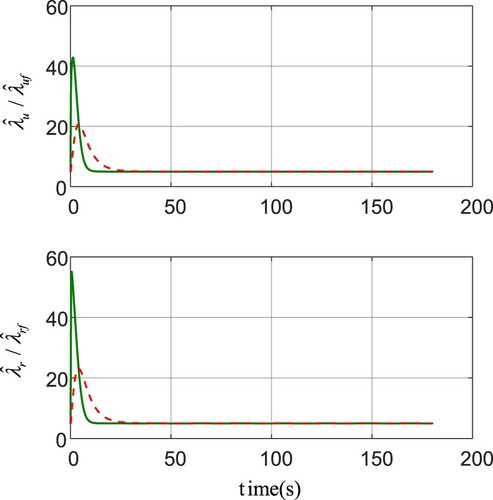
Figure 2–6 have displayed the simulation results. In Figure 2, the formation trajectory under the 2-D planform has been exhibited. It is obvious that despite the existence of time-varying parameterized disturbances and unknown model uncertain terms, the formation could navigate along the reference path with a desired formation configuration, which illustrate the robustness of the proposed control algorithm. Figure 3 demonstrates the velocities on the surge, sway and yaw motion, respectively. Obviously, the velocities of USVs can converge to a satisfactory range rapidly. To reflect the simulation results more intensively, one gives the curves of the tracking errors in Figure 4. Although the length of ship is 38 m, the tracking errors can converge to a small range around zero. In addition, the control efforts (i.e. the propeller forces and the rudder moments) are presented in Figure 5, and the smoothness of the control signals can be guaranteed. Moreover, the adaptive laws ${\hat{\lambda }}_i$ and ${\hat{\lambda }}_{if},i=u,r$ can be found in Figure 6. From the results, one can see that the compensating performance under the LFG technique is with faster convergency ability, which can enable the formation to approach from the initial position to the desired reference path as quickly as possible. Besides, in lieu of updating the burdensome fuzzy weights, only two adaptive learning parameters are required to compensate the system uncertainty and unknown disturbances, which can reduce the computational load of the closed-loop control system.

Figure 2. Trajectory of formation under the 2D plane.

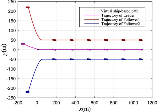
Figure 3. The velocity values of USVs under the proposed algorithm.

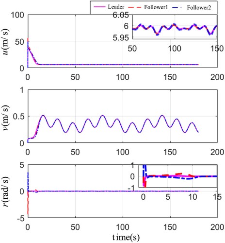
Figure 4. The tracking errors of USVs of the proposed algorithm.

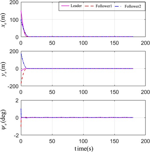
Figure 5. The control efforts of the proposed algorithm.

Figure 6. The adaptive laws: ${\hat{\lambda }}_u$, ${\hat{\lambda }}_r$ (dashed line) and ${\hat{\lambda }}_{uf}$, ${\hat{\lambda }}_{rf}$ (solid line).

5. Conclusion

In this note, the formation problem of underactuated ships under the model uncertainties and unknown parameterized disturbances has been considered. In order to overcome the ‘explosion of complexity’ and ‘curse of dimensionality’ in the traditional Backstepping framework, the MLP and DSC are introduced so that only two fuzzy learning parameters are required to update online rather than the enormous weight matrix, which can reduce the computational burden in the closed-loop control system. Different from the existing DSC methods, the proposed algorithm could derive filter compensating signals to optimize the process of controller design and no filtered errors need to be stabilized in the stability analysis. Furthermore, the stability analysis guarantees SGUUB of all the signals in the closed loop system by using the Lyapunov theory. The simulated experiment has been presented to illustrate the effectiveness of the proposed control scheme. Even though, this work cannot attend to every detail of the control task, e.g. the algorithm may not targetly tackle with the communication between the followers. That would be the further problem to be solved in the following works.

Acknowledgments

The authors would like to express our gratitude to the Editor-in-Chief, the Associate Editor, as well as the anonymous reviewers for the time and effort that had been spent in processing our manuscript.

Data availability statement

The data that support the findings of this study are available from the corresponding author, Guoqing Zhang, upon reasonable request.

Disclosure statement

No potential conflict of interest was reported by the authors.

Additional information

Funding

This paper is partially supported by the National Natural Science Foundation of China [grant numbers 51909018, 51679024, 52171291], the Natural Science Foundation of Liaoning Province [grant numbers 20170520189, 20180520039], the Science and Technology Innovation Foundation of Dalian City [grant number 2019J12GX026], the Fundamental Research Funds for the Central Universities in China [grant number 3132020124].

References

- Do, K. D. (2010). Practical control of underactuated ships. Ocean Engineering, 37(13), 1111–1119. https://doi.org/10.1016/j.oceaneng.2010.04.007
- Fahimi, F. (2007). Sliding-mode formation control for underactuated surface vessels. IEEE Transactions on Robotics, 23(3), 617–622. https://doi.org/10.1109/TRO.2007.898961
- Fossen, T. I. (1998). Guidance and control of ocean vehicles. Wiley.
- Li, J., Zhang, G., Liu, C., & Zhang, W. (2020). COLREGs-constrained adaptive fuzzy event-triggered control for underactuated surface vessels with the actuator failures. IEEE Transactions on Fuzzy Systems. https://doi.org/10.1109/TFUZZ.2020.3028907
- Li, J. H., Lee, P. M., Jun, B. H., & Lim, Y. K. (2008). Point-to-point navigation of underactuated ships. Automatica, 44(12), 3201–3205. https://doi.org/10.1016/j.automatica.2008.08.003
- Li, Y., & Tong, S. (2018). Adaptive fuzzy control with prescribed performance for block-triangular-structued nonlinear systems. IEEE Transactions on Fuzzy Systems, 26(3), 1153–1163. https://doi.org/10.1109/TFUZZ.91
- Li, Y., Tong, S., & Li, T. (2015). Composite adaptive fuzzy output feedback control design for uncertain nonlinear strict-feedback systems with input saturation. IEEE Transactions on Cybernetics, 45(10), 2299–2308. https://doi.org/10.1109/TCYB.2014.2370645
- Li, Y., Tong, S., & Li, T. (2016). Hybrid fuzzy adaptive output feedback control design for MIMO time varying delays uncertain nonlinear systems. IEEE Transactions on Fuzzy Systems, 24(4), 841–853. https://doi.org/10.1109/TFUZZ.2015.2486811
- Liu, C., Wang, D., Zhang, Y., & Meng, X. (2020). Model predictive control for path following and roll stabilization of marine vessels based on neurodynamic optimization. Ocean Engineering, 217(5), 107524. https://doi.org/10.1016/j.oceaneng.2020.107524
- Lu, Y., Zhang, G., Sun, Z., & Zhang, W. (2018). Robust adaptive formation control of underactuated autonomous surface vessels based on mlp and dob. Nonlinear Dynamics, 94(1), 503–519. https://doi.org/10.1007/s11071-018-4374-z
- Peng, Z., Wang, D., Chen, Z., Hu, X., & Lan, W. (2013). Adaptive dynamic surface control for formations of autonomous surface vehicles with uncertain dynamics. IEEE Transactions on Control Systems Technology, 21(2), 513–520. https://doi.org/10.1109/TCST.2011.2181513
- Peng, Z., Wang, D., Li, T., & Han, M. (2020). Output-feedback cooperative formation maneuvering of autonomous surface vehicles with connectivity preservation and collision avoidance. IEEE Transactions on Cybernetics, 50(6), 2527–2535. https://doi.org/10.1109/TCYB.6221036
- Peng, Z., Wang, J., Wang, D., & Han, Q. L. (2021). An overview of recent advances in coordinated control of multiple autonomous surface vehicles. IEEE Transactions on Industrial Informatics, 17(2), 732–745. https://doi.org/10.1109/TII.2020.3004343
- Shojaei, K. (2015). Leader-follower formation control of underactuated autonomous marine surface vehicles with limited torque. Ocean Engineering, 105(6), 196–205. https://doi.org/10.1016/j.oceaneng.2015.06.026
- Tee, K. P., & Ge, S. S. (2006). Control of fully actuated ocean surface vessels using a class of feedforward approximators. IEEE Transactions on Control Systems Technology, 14(4), 750–756. https://doi.org/10.1109/TCST.2006.872507
- Wang, M., Liu, X., & Shi, P. (2011). Adaptive neural control of pure-feedback nonlinear time-delay systems via dynamic surface technique. IEEE Transactions on Systems, Man, and Cybernetics-Part B: Cybernetics, 41(6), 1681–1691. https://doi.org/10.1109/TSMCB.2011.2159111
- Wang, Y., Jiang, B., Wu, Z., Xie, S., & Peng, Y. (2021). Adaptive sliding mode fault-tolerant fuzzy tracking control with application to unmanned marine vehicles. IEEE Transactions on Systems, Man, and Cybernetics: Systems, 51(11), 6691–6700. 10.1109/TSMC.2020.2964808
- Xiang, X., Lapierre, L., & Jouvencel, B. (2010). Guidance based collision free and obstacle avoidance of autonomous vehicles under formation constraints. IFAC Proceedings Volumes, 43(16), 599–604. https://doi.org/10.3182/20100906-3-IT-2019.00103
- Xiang, X., Yu, C., & Zhang, Q. (2017). Robust fuzzy 3d path following for autonomous underwater vehicle subject to uncertainties. Computers and Operations Research, 84(11), 165–177. https://doi.org/10.1016/j.cor.2016.09.017
- Xiao, B., Yang, X., & Huo, X. (2017). A novel disturbance estimation scheme for formation control of ocean surface vessels. IEEE Transactions on Industrial Electronics, 64(6), 4994–5003. https://doi.org/10.1109/TIE.2016.2622219
- Yang, Y., Feng, G., & Li, T. (2004). A combined backstepping and small-gain approach to robust adaptive fuzzy control for strict-feedback nonlinear systems. IEEE Transactions on Systems, Man, and Cybernetics -- Part A: Systems and Humans, 34(3), 406–420. https://doi.org/10.1109/TSMCA.2004.824870
- Yang, Y., & Ren, J. (2003). Adaptive fuzzy robust tracking controller design via small gain approach and its application. IEEE Transactions on Fuzzy System, 11(6), 783–795. https://doi.org/10.1109/TFUZZ.2003.819837
- Zhang, G., Chu, S., Jin, X., & Zhang, W. (2020). Composite neural learning fault-tolerant control for underactuated vehicles with event-triggered input. IEEE Transactions on Cybernetics, 51(5), 2327–2338. https://doi.org/10.1109/TCYB.2020.3005800
- Zhang, G., Zhang, X., & Zheng, Y. (2015). Adaptive neural path-following control for underactuated ships in fields of marine practice. Ocean Engineering, 104(8), 558–567. https://doi.org/10.1016/j.oceaneng.2015.05.013
- Zhou, W., Wang, Y., Ahn, C. K., Chen, J., & Chen, C. (2020). Adaptive fuzzy backstepping-based formation control of unmanned surface vehicles with unknown model nonlinearity and actuator saturation. IEEE Transactions on Vehicular Technology, 69(12), 14749–14762. https://doi.org/10.1109/TVT.25