Distributed recursive fault estimation with binary encoding schemes over sensor networks

Abstract

In this paper, we investigate the distributed recursive fault estimation problem for a class of discrete time-varying systems with binary encoding schemes over a sensor network. The fault signal with zero second-order difference is taken into account to reflect the sensor failures. Since the communication bandwidth in practice is constrained, the binary encoding schemes are exploited to regulate the signal transmission from the neighbouring sensors to the local fault estimator. In addition, due to the influence of channel noises, each bit might change with a small crossover probability. In the presence of sensor faults and bit errors, an upper bound for the estimation error covariance matrix is ensured and minimized at each time step via designing the gain matrices of the estimator. Finally, the effectiveness of the method is verified by a simulation.

Keywords:

• Distributed fault estimation
• sensor network
• stochastic bias
• bit error

1. Introduction

Sensor networks are constitutive of numerous inexpensive wireless devices installed over the environment of interest to transmit the collected data. These devices, called sensor nodes, are typically distributed in space to form a wireless self-organizing network that is capable of processing assignments through information interaction among sensors. With the rapid development of hardware implementation, software development and theoretical research, sensor networks have gained increasing applications in multifarious fields, such as battlefield surveillance, distributed robotics, biomedical health monitoring, traffic control and automatic production, see, e.g. Alippi and Galperti (2008), Dong et al. (2013), Ding et al. (2012), Cong et al. (2021), Geng et al. (2021) and Jia (2021). One of the interesting research themes of sensor networks is how to validly transmit collected data in case of sensor faults. Unlike traditional networks without data sharing, sensor networks have the characteristic of relying on dense deployment and coordination to perform tasks, which have become an ever-growing research concern (Battilotti & Mekhail, 2019; Caballero-Águila et al., 2017; Ge et al., 2019a, 2019b; Lin & Sun, 2019; L. Liu et al., 2021; Liu et al., 2015; Zhao, 2018).

In sensor networks, distributed filtering has always played a key role in numerous areas such as signal processing and control engineering, and plenty of the previous research achievements about distributed filtering algorithms have focused on robustness or stability, see, e.g. Zhang et al. (2017), Zhang et al. (2015) and Zhu et al. (2016). In particular, a novel distributed filter whose available innovations are from not only the individual sensor but also its neighbouring ones according to the given topology has been designed in Ding et al. (2017) with effects from the uniform quantization and the deception attack on the measurement outputs. Furthermore, cooperative information processing mechanism is the core link of distributed filters, that is, each node calculates by using both its own measurement and the information accepted/transmitted from its neighbouring sensors based on the connection topology, which means it is necessary to require the channel to transmit signals safely and accurately. Naturally, the encoding–decoding strategy for signal transmission, which facilitates the data safety and reduces the network resource occupation, has attracted much attention quickly (Cao et al., 2021; Wang et al., 2018).

The encoding and decoding scheme is a popular direction in recent years to avoid the trouble that the signal is easy to be monitored in the transmission process. Compared with other schemes, the binary encoding schemes (BESs), using the binary bit string to encode, have merits of little network resource consumption and higher anti-interference ability (S. Hu et al., 2020; Xu et al., 2020). In general situations, random bit errors may occur inevitably considering the existence of channel noises during the course of digital signal transmission, in which the binary bit is changed to the other value. When bit errors occur, the decoded signal has a certain deviation from the encoded signal, and such a distinction would result in that the system performance degrades. Recently, initial research attention has been paid to the analysis of the influence from random bit errors on the estimation performance, see Leung et al. (2015), Liu and Wang (2021), Morrow and Lehnert (1989) and Zou et al. (2021). For instance, the moving-horizon state estimation problem has been investigated in Liu and Wang (2021) of discrete-time linear dynamic network, in which the BES has been exploited during the signal transmission. Nevertheless, the relevant work has rarely been considered for the sensor network. Therefore, one of the motivations of this paper is to investigate the synthesis problem for systems under BESs over sensor networks.

Actually, due to the actual needs of production process, fault diagnosis and fault-tolerant control issues have stirred many researchers' attention, which have been tackled with for various systems in a large number of publications, see, e.g. Li and Yang (2017), Ye et al. (2017), Selvaraj et al. (2018), J. Li et al. (2019), Gao et al. (2019) and Song et al. (2020). For example, the neural networks-based adaptive finite-time fault-tolerant control strategy has been investigated in Liu et al. (2019) for a class of strict-feedback switched nonlinear systems. In Y. Li et al. (2019), the fault-tolerant topic has been studied for SISO nonlinear systems by using the observer-based adaptive fuzzy optimal control. In Chen and Jiang (2020), the matter of fault detection and diagnosis has been handled for traction systems in high-speed trains. As is well known, the prerequisite for accurate fault diagnosis is fault estimation, because it could effectively provide the shape and size of the defect. Noting that the failure of one sensor node may inevitably destroy the accuracy of the whole sensor network because of its distributed transmission characteristics, then it is imperative to acquire the fault information of sensor. However, on account of the complexity of math, distributed recursive estimate of faults over sensor networks has not been fully coped with, needless to say that BESs are also utilized, and this is the other motivation in this paper.

In this paper, we plan to estimate both the sensor faults and the state for time-varying systems over sensor networks with binary encoding schemes. The main contributions of this paper are emphasized in the following three aspects: (1) the problem of distributed recursive fault estimation is examined of time-varying systems with BESs over sensor networks; (2) the situation under consideration is complicated concerning time-varying parameters, sensor faults with zero second-order difference and random error codes; and (3) the upper limit of the estimation error (EE) covariance matrix is calculated and minimized afterwards by designing appropriate estimator parameters.

The remainder of this paper is outlined as follows. In Section 2, the discrete time-varying sensor network system is formulated with faults under binary encoding schemes. The distributed recursive fault estimation problem is carried out in Section 3. A simulation example is conducted in Section 4 and conclusion is given in Section 5.

Notation: In this paper, ${\mathbb{R}}^m$ stands for the m-dimensional Euclidean space. A>0 represents that A is a positive definite symmetric matrix. For a square matrix B, $\mathrm{Trace}(B)$ illustrates the trace of B. $\mathbb{E}\{a\}$ and $\mathrm{Var}\{a\}$ show the expectation and the variance of the random variable a, respectively. $\mathrm{Cov}\{X\}$ means the covariance of the random vector X. $\mathrm{Prob}\{\cdot \}$ denotes the occurrence probability of the event ‘·’. $\mathbf{0}$ stands for a vector whose entries are all 0.

2. Problem formulation and preliminaries

In this paper, we are concerned with a sensor network containing M sensor nodes, whose topology is depicted by a specified directed graph $\mathbf{G}=(\mathrm{\Theta },\mathrm{\Xi },\mathrm{\Lambda })$ of order M with the set of nodes $\mathrm{\Theta }=\{1,2,\dots ,M\}$, the set of edges $\mathrm{\Xi }\subseteq \mathrm{\Theta }\times \mathrm{\Theta }$, and the weighted adjacency matrix $\mathrm{\Lambda }=[a_{ji}{]}_{M\times M}$ with adjacency elements $a_{ji}\ge 0$. An edge of $\mathbf{G}$ is represented by pair $(i,j)$. The adjacency elements associated with the edges of the graph are positive, i.e. $a_{ji}>0⟺(j,i)\in \mathrm{\Xi }$, which means that there exists the information transmission from sensor j to i. The set of neighbours of node i is expressed by ${\mathbf{N}}_i=\{j\in \mathrm{\Theta }:a_{ji}>0\}$ ($j\ne i$). The in-degree of node i is illustrated via ${\mathrm{\Im }}_i^{\mathrm{in}}=\sum _{j\in {\mathbf{N}}_i}{a}_{ji}$. In this paper, suppose ${\mathrm{\Im }}_i^{\mathrm{in}}\ne 0$ for all nodes.

Consider a class of discrete time-varying systems as follows: (1) $x_{s+1}=A_s{x}_s+E_s{\omega }_s$(1) where $x_s\in {\mathbb{R}}^{o_x}$ is the system state, ${\omega }_s\in {\mathbb{R}}^{o_{\omega }}$ is the process noise which is a bounded stochastic noise sequence with zero mean and covariance $W_s>0$. $A_s$ and $E_s$ are known matrices with proper dimensions.

The measurement of the ith ($i=1,2,\dots ,M$) sensor node is described by (2) $y_{i,s}=C_{0,s}{x}_s+H_{0,s}{f}_{i,s}+D_{i,s}{\nu }_{i,s}$(2) where $y_{i,s}={\left[\begin{array}{cccc}{y}_{i1,s}& y_{i2,s}& \cdots & y_{i{o}_y,s}\end{array}\right]}^T\in {\mathbb{R}}^{o_y}$ is the output of sensor i, $f_{i,s}\in {\mathbb{R}}^{o_f}$ means the addictive sensor fault and ${\nu }_{i,s}\in {\mathbb{R}}^{o_{\nu }}$ is the measurement noise which is a bounded stochastic noise sequence with zero mean and covariance $Q_{i,s}>0$. $C_{0,s}$, $H_{0,s}$ and $D_{i,s}$ are given matrices with proper dimensions.

We denote $f_{i,s}^{[0]}\triangleq f_{i,s}$ and $f_{i,s}^{[p]}\triangleq f_{i,s+1}^{[p-1]}-f_{i,s}^{[p-1]}$ $(p\ge 1)$ with $f_{i,0}=\mathbf{0}$. Noting that no information is known on the dynamics of the sensor faults, a stochastic bias ${\psi }_{i,s}$ is taken into consideration in the first-order difference of the sensor faults $f_{i,s}$ with a large covariance, that is, (3) $f_{i,s+1}^{[1]}=f_{i,s}^{[1]}+{\psi }_{i,s}$(3) where ${\psi }_{i,s}\in {\mathbb{R}}^{o_f}$ is the zero-mean bounded stochastic noise sequence whose covariance is $R_{i,s}>0$ (Y. Liu et al., 2021). Assume that the random vectors ${\omega }_s$, ${\nu }_{i,s}$ and ${\psi }_{i,s}$ are mutually uncorrelated.

Remark 2.1

If ${\psi }_{i,s}$ is not considered in (3(3) $f_{i,s+1}^{[1]}=f_{i,s}^{[1]}+{\psi }_{i,s}$(3) ), we have $f_{i,s+1}^{[1]}=f_{i,s}^{[1]}$ (i.e. $f_{i,s}^{[1]}=const$) which may not reflect the inflection point and the perturbation in the first-order difference of a fault signal. The stochastic-bias-expression (3(3) $f_{i,s+1}^{[1]}=f_{i,s}^{[1]}+{\psi }_{i,s}$(3) ) is not limited to describing sudden faults in the inertial sensor (accelerometer) of intelligent vehicles.

Let ${\overline{x}}_{i,s}\triangleq {\left[\begin{array}{ccc}{x}_s^T& f_{i,s}^T& (f_{i,s}^{[1]}{)}^T\end{array}\right]}^T$. The dynamics of the augmented state is acquired from (1(1) $x_{s+1}=A_s{x}_s+E_s{\omega }_s$(1) )–(3(3) $f_{i,s+1}^{[1]}=f_{i,s}^{[1]}+{\psi }_{i,s}$(3) ) as follows: (4) $\begin{array}{rl}{\overline{x}}_{i,s+1}& ={\overline{A}}_s{\overline{x}}_{i,s}+{\overline{E}}_s{\overline{\omega }}_{i,s}\end{array}$(4) (5) $\begin{array}{rl}{y}_{i,s}& ={\overline{C}}_{0,s}{\overline{x}}_{i,s}+D_{i,s}{\nu }_{i,s}\end{array}$(5) where $\begin{array}{rl}{\overline{A}}_s& \triangleq \left[\begin{array}{ccc}{A}_s& 0& 0\\ 0& I& I\\ 0& 0& I\end{array}\right],{\overline{E}}_s\triangleq \left[\begin{array}{cc}{E}_s& 0\\ 0& 0\\ 0& I\end{array}\right],\\ {\overline{\omega }}_{i,s}& \triangleq \left[\begin{array}{c}{\omega }_s\\ {\psi }_{i,s}\end{array}\right],{\overline{C}}_{0,s}\triangleq \left[\begin{array}{ccc}{C}_{0,s}& H_{0,s}& 0\end{array}\right].\end{array}$It is known that $\mathbb{E}\{{\overline{\omega }}_{i,s}\}=\mathbf{0}$ and $\mathrm{Cov}\{{\overline{\omega }}_{i,s}\}={\overline{W}}_{i,s}$ with ${\overline{W}}_{i,s}=\mathrm{diag}\{W_s,R_{i,s}\}$.

In this paper, the binary encoding schemes are employed during the signal transmission from the neighbouring sensors to the local fault estimator (Liu & Wang,2021). Due to the limitation of the actual communication bandwidth, only a restricted bit budget can be used to encode the signal on the communication channel, in which the use of a quantization function is required to preprocess the signal. In this paper, the original signal $y_{i,s}$ is coded into a binary bit sequence of finite length. The binary bit sequence is transmitted to the remote fault estimator for subsequent manipulation through a memoryless binary symmetric channel.

Assume that the range of the scalar signal $y_{i\ell ,s}\in \mathbb{R}$ is $[-b_{i\ell },b_{i\ell }]$ ($\ell =1,2,\dots ,o_y$) at the moment of s, where $b_{i\ell }>0$ is a scalar that depends on the application. Use a binary encoder to convert the signal $y_{i\ell ,s}$ into a binary bit string of length N.

For this situation, the whole range $[-b_{i\ell },b_{i\ell }]$ is divided into $2^N-1$ segments, and the interval length is given as follows: (6) ${ϵ}_{i\ell }=\frac{2b_{i\ell }}{2^N-1}.$(6) Let the uniformly spaced $2^N$ points (two endpoints and internal points inside) be represented by ${\mathcal{P}}_{i\ell }\triangleq \{{\mathrm{\wp }}_{i\ell }^{(1)},{\mathrm{\wp }}_{i\ell }^{(2)},{\mathrm{\wp }}_{i\ell }^{(3)},\dots ,{\mathrm{\wp }}_{i\ell }^{(2^N)}\}$where (7) ${\mathrm{\wp }}_{i\ell }^{(\iota )}\triangleq -b_{i\ell }+(\iota -1){ϵ}_{i\ell },\iota =1,2,\dots ,2^N.$(7) A stochastic quantization function ${\mathcal{Q}}_{i\ell ,s}$ is employed to preprocess the signal $y_{i\ell ,s}$ as follows: (8) ${\mathcal{Q}}_{i\ell ,s}:y_{i\ell ,s}\to m_{i\ell }(s,y_{i\ell ,s},N)$(8) where $m_{i\ell }(s,y_{i\ell ,s},N)$ is the quantized output (Aysal et al., 2007). When ${\mathrm{\wp }}_{i\ell }^{(\iota )}\le y_{i\ell ,s}\le {\mathrm{\wp }}_{i\ell }^{(\iota +1)}$, output $m_{i\ell }(s,y_{i\ell ,s},N)$ is generated according to the following probability: (9) $\begin{array}{rl}& \mathrm{Prob}\{m_{i\ell }(s,y_{i\ell ,s},N)={\mathrm{\wp }}_{i\ell }^{(\iota )}\}=1-p_{i\ell ,s},\\ & \mathrm{Prob}\{m_{i\ell }(s,y_{i\ell ,s},N)={\mathrm{\wp }}_{i\ell }^{(\iota +1)}\}=p_{i\ell ,s}\end{array}$(9) where $p_{i\ell ,s}\triangleq \frac{y_{i\ell ,s}-{\mathrm{\wp }}_{i\ell }^{(\iota )}}{{ϵ}_{i\ell }}$ and $0\le p_{i\ell ,s}\le 1$. In this case, we only know the probability of $m_{i\ell }(s,y_{i\ell ,s},N)={\mathrm{\wp }}_{i\ell }^{(\iota )}$ (or ${\mathrm{\wp }}_{i\ell }^{(\iota +1)}$) rather than the specific value, which depends on the value of $y_{i\ell ,s}$.

Define $r_{i\ell ,s}\triangleq m_{i\ell }(s,y_{i\ell ,s},N)-y_{i\ell ,s}$ as the quantization error. In terms of (9(9) $\begin{array}{rl}& \mathrm{Prob}\{m_{i\ell }(s,y_{i\ell ,s},N)={\mathrm{\wp }}_{i\ell }^{(\iota )}\}=1-p_{i\ell ,s},\\ & \mathrm{Prob}\{m_{i\ell }(s,y_{i\ell ,s},N)={\mathrm{\wp }}_{i\ell }^{(\iota +1)}\}=p_{i\ell ,s}\end{array}$(9) ), we see that $r_{i\ell ,s}$ is a stochastic noise conforming to the Bernoulli distribution as follows: (10) $\begin{array}{rl}& \mathrm{Prob}\{r_{i\ell ,s}=-p_{i\ell ,s}{ϵ}_{i\ell }\}=1-p_{i\ell ,s},\\ & \mathrm{Prob}\{r_{i\ell ,s}=(1-p_{i\ell ,s}){ϵ}_{i\ell }\}=p_{i\ell ,s}.\end{array}$(10) It is acquired that (11) $\mathbb{E}\{r_{i\ell ,s}\}=0$(11) and (12) $\mathrm{Var}\{r_{i\ell ,s}\}\le \frac{{ϵ}_{i\ell }^2}{4}.$(12) Since the quantization of $y_{i\ell ,s}$ is performed independently, we see that $r_{i\ell ,s}$ are mutually independent.

An encoding function ${\mathcal{N}}_{i\ell ,s}$ is utilized to denote the output $m_{i\ell }(s,y_{i\ell ,s},N)$ based on binary bits as follows: (13) ${\mathcal{N}}_{i\ell ,s}:m_{i\ell }(s,y_{i\ell ,s},N)\to B_{i\ell ,s}$(13) where $B_{i\ell ,s}\triangleq \{{\hslash }_{i\ell ,s}^{(1)},{\hslash }_{i\ell ,s}^{(2)},\dots ,{\hslash }_{i\ell ,s}^{(N)}\}$ (${\hslash }_{i\ell ,s}^{(\varsigma )}\in \{0,1\},\varsigma =1,2,\dots ,N$) represents the binary bit string, which is acquired by the following expression: (14) $m_{i\ell }(s,y_{i\ell ,s},N)=-b_{i\ell }+\sum _{\varsigma =1}^N{\hslash }_{i\ell ,s}^{(\varsigma )}{2}^{\varsigma -1}{ϵ}_{i\ell }.$(14) The next step is to transmit the binary bit sequence $B_{i\ell ,s}$ through a memoryless binary symmetric channel, where each bit may change with a small probability (crossover probability) due to channel noises. Therefore the received bit sequence is defined as $\begin{array}{rl}& Y_{i\ell ,s}\triangleq \{{\lambda }_{i\ell ,s}^{(1)},{\lambda }_{i\ell ,s}^{(2)},\dots ,{\lambda }_{i\ell ,s}^{(N)}\},\\ & {\lambda }_{i\ell ,s}^{(\varsigma )}\in \{0,1\},\varsigma =1,2,\dots ,N\end{array}$where ${\lambda }_{i\ell ,s}^{(\varsigma )}={\vartheta }_{i\ell ,s}^{(\varsigma )}(1-{\hslash }_{i\ell ,s}^{(\varsigma )})+(1-{\vartheta }_{i\ell ,s}^{(\varsigma )}){\hslash }_{i\ell ,s}^{(\varsigma )}$ indicating the ςth bit is with (15) ${\vartheta }_{i\ell ,s}^{(\varsigma )}=\{\begin{array}{ll}1,& \text{bit error occurs,}\\ 0,& \text{bit error does not occur}.\end{array}$(15) The probabilities of ${\vartheta }_{i\ell ,s}^{(\varsigma )}$ are as follows: $\mathrm{Prob}\{{\vartheta }_{i\ell ,s}^{(\varsigma )}=1\}=q,\mathrm{Prob}\{{\vartheta }_{i\ell ,s}^{(\varsigma )}=0\}=1-q$where $q\in [0,1]$ represents the crossover probability.

For the convenience of analysis, we introduce the following assumption.

Assumption 2.1

In (15(15) ${\vartheta }_{i\ell ,s}^{(\varsigma )}=\{\begin{array}{ll}1,& \text{bit error occurs,}\\ 0,& \text{bit error does not occur}.\end{array}$(15) ), ${\vartheta }_{i\ell ,s}^{(\varsigma )}$ $(\varsigma =1,2,\dots ,N)$ are mutually independent and identically distributed.

A decoding function ${\mathcal{D}}_{i\ell ,s}$ is employed to decode the received bit string $Y_{i\ell ,s}$ as follows: (16) ${\mathcal{D}}_{i\ell ,s}:Y_{i\ell ,s}\to z_{i\ell }(s,y_{i\ell ,s},N)$(16) where $z_{i\ell }(s,y_{i\ell ,s},N)$ represents the restored signals after transmission with the following expression: (17) $z_{i\ell }(s,y_{i\ell ,s},N)=-b_{i\ell }+\sum _{\varsigma =1}^N{\lambda }_{i\ell ,s}^{(\varsigma )}{2}^{\varsigma -1}{ϵ}_{i\ell }.$(17) We see that ${\lambda }_{i\ell ,s}^{(\varsigma )}$ are mutually independent as well as $z_{i\ell }(s,y_{i\ell ,s},N)$. Lemma 2.1 is given to facilitate later analysis.

Lemma 2.1

Liu & Wang, 2021

Suppose the signal $m_{i\ell }(s,y_{i\ell ,s},N)$ is transmitted through a memoryless binary symmetric channel with crossover probability q. The obtained signal is $z_{i\ell }(s,y_{i\ell ,s},N)$, and its expectation and variance are (18) $\mathbb{E}\{z_{i\ell }(s,y_{i\ell ,s},N)\}=(1-2q)m_{i\ell }(s,y_{i\ell ,s},N)$(18) and (19) $\mathrm{Var}\{z_{i\ell }(s,y_{i\ell ,s},N)\}=b_{i\ell }^2\sigma$(19) where $\sigma \triangleq \frac{4q(1-q)(2^{2N}-1)}{3(2^N-1{)}^2}$ and the expectation is related to the random variable ${\vartheta }_{i\ell ,s}^{(\varsigma )}$.

Let $\begin{array}{rl}{m}_i(s,y_{i,s},N)& \triangleq [\begin{array}{cc}{m}_{i1}(s,y_{i1,s},N)& m_{i2}(s,y_{i2,s},N)\end{array}\\ & {\begin{array}{cc}\cdots & m_{i{o}_y}(s,y_{i{o}_y,s},N)\end{array}]}^T,\\ r_{i,s}& \triangleq {\left[\begin{array}{cccc}{r}_{i1,s}& r_{i2,s}& \cdots & r_{i{o}_y,s}\end{array}\right]}^T,\\ z_i(s,y_{i,s},N)& \triangleq [\begin{array}{cc}{z}_{i1}(s,y_{i1,s},N)& z_{i2}(s,y_{i2,s},N)\end{array}\\ & {\begin{array}{cc}\cdots & z_{i{o}_y}(s,y_{i{o}_y,s},N)\end{array}]}^T.\end{array}$In terms of (11(11) $\mathbb{E}\{r_{i\ell ,s}\}=0$(11) ), (12(12) $\mathrm{Var}\{r_{i\ell ,s}\}\le \frac{{ϵ}_{i\ell }^2}{4}.$(12) ), (18(18) $\mathbb{E}\{z_{i\ell }(s,y_{i\ell ,s},N)\}=(1-2q)m_{i\ell }(s,y_{i\ell ,s},N)$(18) ) and (19(19) $\mathrm{Var}\{z_{i\ell }(s,y_{i\ell ,s},N)\}=b_{i\ell }^2\sigma$(19) ), it is obtained that (20) $\begin{array}{rl}& \mathbb{E}\{r_{i,s}\}=\mathbf{0},\end{array}$(20) (21) $\begin{array}{rl}& \mathrm{Cov}\{r_{i,s}\}\le \frac{{ϵ}_i}{4},\end{array}$(21) (22) $\begin{array}{rl}& \mathbb{E}\{z_i(s,y_{i,s},N)\}=(1-2q)m_i(s,y_{i,s},N),\end{array}$(22) (23) $\begin{array}{rl}& \mathrm{Cov}\{z_i(s,y_{i,s},N)\}={\hat{b}}_i\otimes \sigma \end{array}$(23) where ${ϵ}_i\triangleq \mathrm{diag}\{{ϵ}_{i1}^2,{ϵ}_{i2}^2,\dots ,{ϵ}_{i{o}_y}^2\}$ and ${\hat{b}}_i\triangleq \mathrm{diag}\{b_{i1}^2,b_{i2}^2,\dots ,b_{i{o}_y}^2\}$.

Based on (20(20) $\begin{array}{rl}& \mathbb{E}\{r_{i,s}\}=\mathbf{0},\end{array}$(20) )–(23(23) $\begin{array}{rl}& \mathrm{Cov}\{z_i(s,y_{i,s},N)\}={\hat{b}}_i\otimes \sigma \end{array}$(23) ), we see that the received signals $z_i(s,y_{i,s},N)$ suffer from certain degree of distortions unavoidably in comparison with the encoded signals $m_i(s,y_{i,s},N)$. Then, we employ the following recovered measurements for the sake of compensating for the distortions: (24) ${\tilde{y}}_{i,s}=\frac{1}{1-2q}{z}_i(s,y_{i,s},N).$(24) It is noted that $\mathbb{E}\{{\tilde{y}}_{i,s}\}=m_i(s,y_{i,s},N)$. Then, the equivalent noise coming from bit errors in binary symmetric channels is represented by (25) ${\tilde{m}}_{i,s}={\tilde{y}}_{i,s}-m_i(s,y_{i,s},N).$(25) According to (22(22) $\begin{array}{rl}& \mathbb{E}\{z_i(s,y_{i,s},N)\}=(1-2q)m_i(s,y_{i,s},N),\end{array}$(22) )–(25(25) ${\tilde{m}}_{i,s}={\tilde{y}}_{i,s}-m_i(s,y_{i,s},N).$(25) ), we know that $\mathbb{E}\{{\tilde{m}}_{i,s}\}=\mathbf{0}$ and $\mathrm{Cov}\{{\tilde{m}}_{i,s}\}=\frac{1}{(1-2q{)}^2}\mathrm{Cov}\{z_i(s,y_{i,s},N)\}={\mathrm{\Pi }}_i$ with ${\mathrm{\Pi }}_i=\frac{1}{(1-2q{)}^2}({\hat{b}}_i\otimes \sigma )$. It should be mentioned that ${\tilde{m}}_{i,s}$ are mutually independent.

Combining (25(25) ${\tilde{m}}_{i,s}={\tilde{y}}_{i,s}-m_i(s,y_{i,s},N).$(25) ) with $r_{i,s}=m_i(s,y_{i,s},N)-y_{i,s}$, one has the expression of ${\tilde{y}}_{i,s}$ as follows: (26) ${\tilde{y}}_{i,s}=y_{i,s}+r_{i,s}+{\tilde{m}}_{i,s}.$(26)

Remark 2.2

In this paper, the BES is introduced in the signal transmission process from neighbouring sensors to the local sensor (also the local fault estimator). In the binary symmetric channel, the unavoidable channel noises would probably result in the bit changing from 0 to 1 (or from 1 to 0). Then, we utilize a Bernoulli distributed random sequence with a known probability distribution to reflect and characterize the flipping case of binary bit in practical situations. Furthermore, in (26(26) ${\tilde{y}}_{i,s}=y_{i,s}+r_{i,s}+{\tilde{m}}_{i,s}.$(26) ), the actual received signal from the neighbouring sensor of the local fault estimator is expressed by using the output signal $y_{i,s}$, the quantization error $r_{i,s}$ and the noise equivalent to the influence of the bit error ${\tilde{m}}_{i,s}$. It is worth mentioning that such a description will facilitate the construction of the estimator afterwards.

Let ${\hat{x}}_{i,s+1|s}$ and ${\hat{x}}_{i,s+1|s+1}$ be the one-step prediction and estimate of the system state at the ith sensor node, respectively. In this paper, we are devoted to designing the following distributed estimator (Ding et al., 2017): (27) $\begin{array}{rl}{\hat{x}}_{i,s+1|s}& ={\overline{A}}_s{\hat{x}}_{i,s|s}\end{array}$(27) (28) $\begin{array}{rl}{\hat{x}}_{i,s+1|s+1}& ={\hat{x}}_{i,s+1|s}+{\mathrm{\Im }}_i^{\mathrm{in}}{G}_{i,s+1}(m_i(s+1,y_{i,s+1},N)\\ & -{\overline{C}}_{0,s+1}{\hat{x}}_{i,s+1|s})+K_{i,s+1}\sum _{j\in {\mathbf{N}}_i}{a}_{ji}({\tilde{y}}_{j,s+1}\\ & -{\overline{C}}_{0,s+1}{\hat{x}}_{i,s+1|s})\end{array}$(28) where $G_{i,s+1}$ and $K_{i,s+1}$ are the estimator gain matrices to be designed.

Remark 2.3

In a sensor network, a sensor node presents characteristics including the cheap cost and the information acquisition from neighbouring sensors, which is a heated topic among researchers. Considering the distributed estimation issue over sensor networks, the information that the local estimator gets is generally two parts. One part is the self-measuring signal, which is obtained directly without network transmission due to the fact that the sensor node and its own estimator are physically integrated together. The other part is the signal received from neighbouring sensors via the network transmission. Correspondingly, in the estimator structure (28(28) $\begin{array}{rl}{\hat{x}}_{i,s+1|s+1}& ={\hat{x}}_{i,s+1|s}+{\mathrm{\Im }}_i^{\mathrm{in}}{G}_{i,s+1}(m_i(s+1,y_{i,s+1},N)\\ & -{\overline{C}}_{0,s+1}{\hat{x}}_{i,s+1|s})+K_{i,s+1}\sum _{j\in {\mathbf{N}}_i}{a}_{ji}({\tilde{y}}_{j,s+1}\\ & -{\overline{C}}_{0,s+1}{\hat{x}}_{i,s+1|s})\end{array}$(28) ), $m_i(s+1,y_{i,s+1},N)$ and ${\tilde{y}}_{j,s+1}$ ($j\in {\mathbf{N}}_i$) describe the measurement signal from the local node and that from the neighbouring nodes under the BES, respectively.

Define $e_{i,s+1|s}\triangleq {\overline{x}}_{i,s+1}-{\hat{x}}_{i,s+1|s}$ and $e_{i,s+1|s+1}\triangleq {\overline{x}}_{i,s+1}-{\hat{x}}_{i,s+1|s+1}$ as the prediction error and the estimation error. The covariance matrices of the prediction error and the estimation error are indicated by $P_{i,s+1|s}\triangleq \mathbb{E}\{e_{i,s+1|s}{e}_{i,s+1|s}^T\}$ and $P_{i,s+1|s+1}\triangleq \mathbb{E}\{e_{i,s+1|s+1}{e}_{i,s+1|s+1}^T\}$, respectively. Our objectives of this paper are listed as follows:

• an upper bound for the estimation error covariance matrix $P_{i,s+1|s+1}$ is to be found for the augmented system (4(4) $\begin{array}{rl}{\overline{x}}_{i,s+1}& ={\overline{A}}_s{\overline{x}}_{i,s}+{\overline{E}}_s{\overline{\omega }}_{i,s}\end{array}$(4) );

• the obtained upper bound for $P_{i,s+1|s+1}$ is minimized at each time step s by appropriately designing the gain matrices of the estimator (27(27) $\begin{array}{rl}{\hat{x}}_{i,s+1|s}& ={\overline{A}}_s{\hat{x}}_{i,s|s}\end{array}$(27) )–(28(28) $\begin{array}{rl}{\hat{x}}_{i,s+1|s+1}& ={\hat{x}}_{i,s+1|s}+{\mathrm{\Im }}_i^{\mathrm{in}}{G}_{i,s+1}(m_i(s+1,y_{i,s+1},N)\\ & -{\overline{C}}_{0,s+1}{\hat{x}}_{i,s+1|s})+K_{i,s+1}\sum _{j\in {\mathbf{N}}_i}{a}_{ji}({\tilde{y}}_{j,s+1}\\ & -{\overline{C}}_{0,s+1}{\hat{x}}_{i,s+1|s})\end{array}$(28) ) with the measurements of the sensor itself and its neighbours conforming to the topology information of sensor networks.

3. Main results

In this part, we are to design estimator (27(27) $\begin{array}{rl}{\hat{x}}_{i,s+1|s}& ={\overline{A}}_s{\hat{x}}_{i,s|s}\end{array}$(27) )–(28(28) $\begin{array}{rl}{\hat{x}}_{i,s+1|s+1}& ={\hat{x}}_{i,s+1|s}+{\mathrm{\Im }}_i^{\mathrm{in}}{G}_{i,s+1}(m_i(s+1,y_{i,s+1},N)\\ & -{\overline{C}}_{0,s+1}{\hat{x}}_{i,s+1|s})+K_{i,s+1}\sum _{j\in {\mathbf{N}}_i}{a}_{ji}({\tilde{y}}_{j,s+1}\\ & -{\overline{C}}_{0,s+1}{\hat{x}}_{i,s+1|s})\end{array}$(28) ), and the needed lemmas are listed below to provide convenience for discussion.

Lemma 3.1

Ding et al., 2017

Assume that $W=W^T>0$, ${\mathrm{{\rm Y}}}_s(W)={\mathrm{{\rm Y}}}_s^T(W)\in R^{l\times l}$ and ${\mathrm{\Omega }}_s(W)={\mathrm{\Omega }}_s^T(W)\in R^{l\times l}$. If there is $V=V^T>W$ satisfying (29) ${\mathrm{{\rm Y}}}_s(V)\ge {\mathrm{{\rm Y}}}_s(W),{\mathrm{\Omega }}_s(V)\ge {\mathrm{{\rm Y}}}_s(V)$(29) then the solutions ${\mathrm{\Gamma }}_s$ and ${\mathrm{\Pi }}_s$ to the difference equations below: (30) ${\mathrm{\Gamma }}_{s+1}={\mathrm{{\rm Y}}}_s({\mathrm{\Gamma }}_s),{\mathrm{\Pi }}_{s+1}={\mathrm{\Omega }}_s({\mathrm{\Pi }}_s),{\mathrm{\Gamma }}_0={\mathrm{\Pi }}_0>0$(30) guarantee that ${\mathrm{\Gamma }}_s\le {\mathrm{\Pi }}_s$.

Lemma 3.2

Y. Liu et al., 2021

For any two vectors $z,o\in {\mathbb{R}}^n$, the inequality (31) $z{o}^T+o{z}^T\le \epsilon z{z}^T+{\epsilon }^{-1}o{o}^T$(31) holds where $\epsilon >0$ is a constant scalar.

Lemma 3.3

Y. Liu et al., 2021

The partial derivatives of the trace satisfy $\begin{array}{rl}& \frac{\mathrm{\partial }\mathrm{Trace}(MKN)}{\mathrm{\partial }K}=M^T{N}^T,\\ & \frac{\mathrm{\partial }\mathrm{Trace}(M{K}^{T}N)}{\mathrm{\partial }K}=NM,\\ & \frac{\mathrm{\partial }\mathrm{Trace}(MKN{K}^{T}X)}{\mathrm{\partial }K}=M^T{X}^{T}K{N}^T+XMKN.\end{array}$

For promoting subsequent discussion, we specify the following symbols: $\begin{array}{rl}{\gimel }_s& \triangleq {\left[\begin{array}{cccc}{\gimel }_{1,s}^T& {\gimel }_{2,s}^T& \cdots & {\gimel }_{M,s}^T\end{array}\right]}^T(\gimel =\overline{x},\overline{\omega },\nu ,r,\tilde{m}),\\ D_s& \triangleq \mathrm{diag}\{D_{1,s},D_{2,s},\dots ,D_{M,s}\},\\ {\overline{C}}_s& \triangleq \mathrm{diag}\{\underset{M}{\underbrace{{\overline{C}}_{0,s},{\overline{C}}_{0,s},\dots ,{\overline{C}}_{0,s}}}\}.\end{array}$Considering (4(4) $\begin{array}{rl}{\overline{x}}_{i,s+1}& ={\overline{A}}_s{\overline{x}}_{i,s}+{\overline{E}}_s{\overline{\omega }}_{i,s}\end{array}$(4) ), (5(5) $\begin{array}{rl}{y}_{i,s}& ={\overline{C}}_{0,s}{\overline{x}}_{i,s}+D_{i,s}{\nu }_{i,s}\end{array}$(5) ) and (26(26) ${\tilde{y}}_{i,s}=y_{i,s}+r_{i,s}+{\tilde{m}}_{i,s}.$(26) )–(28(28) $\begin{array}{rl}{\hat{x}}_{i,s+1|s+1}& ={\hat{x}}_{i,s+1|s}+{\mathrm{\Im }}_i^{\mathrm{in}}{G}_{i,s+1}(m_i(s+1,y_{i,s+1},N)\\ & -{\overline{C}}_{0,s+1}{\hat{x}}_{i,s+1|s})+K_{i,s+1}\sum _{j\in {\mathbf{N}}_i}{a}_{ji}({\tilde{y}}_{j,s+1}\\ & -{\overline{C}}_{0,s+1}{\hat{x}}_{i,s+1|s})\end{array}$(28) ), the error system dynamics is acquired as follows: (32) $\begin{array}{rl}{e}_{i,s+1|s}& ={\overline{A}}_s{e}_{i,s|s}+{\overline{E}}_s{\overline{\omega }}_{i,s},\end{array}$(32) (33) $\begin{array}{rl}{e}_{i,s+1|s+1}& ={\mathrm{\Phi }}_{i,s+1}{e}_{i,s+1|s}\\ & +K_{i,s+1}(({\mathcal{Z}}_i\otimes I)-({\mathcal{A}}_i\otimes I)){\overline{C}}_{s+1}{\overline{x}}_{s+1}\\ & -(G_{i,s+1}({\mathcal{Z}}_i\otimes I)+K_{i,s+1}({\mathcal{A}}_i\otimes I))D_{s+1}{\nu }_{s+1}\\ & -(G_{i,s+1}({\mathcal{Z}}_i\otimes I)+K_{i,s+1}({\mathcal{A}}_i\otimes I))r_{s+1}\\ & -K_{i,s+1}({\mathcal{A}}_i\otimes I){\tilde{m}}_{s+1}\end{array}$(33) where $\begin{array}{rl}& {\mathrm{\Phi }}_{i,s+1}\triangleq I-{\mathrm{\Im }}_i^{\mathrm{in}}{G}_{i,s+1}{\overline{C}}_{0,s+1}-{\mathrm{\Im }}_i^{\mathrm{in}}{K}_{i,s+1}{\overline{C}}_{0,s+1},\\ & {\mathcal{Z}}_i\triangleq [\underset{i-1}{\underbrace{0\cdots 0}}{\mathrm{\Im }}_i^{\mathrm{in}}\underset{M-i}{\underbrace{0\cdots 0}}],\\ & {\mathcal{A}}_i\triangleq [{\overline{a}}_j^{(i)}{]}_{1\times M}=\{\begin{array}{ll}{\overline{a}}_j^{(i)}=a_{ji},& j\in {\mathbf{N}}_i,\\ {\overline{a}}_j^{(i)}=0,& j\notin {\mathbf{N}}_i.\end{array}\end{array}$From (4(4) $\begin{array}{rl}{\overline{x}}_{i,s+1}& ={\overline{A}}_s{\overline{x}}_{i,s}+{\overline{E}}_s{\overline{\omega }}_{i,s}\end{array}$(4) ), we acquire (34) ${\overline{x}}_{s+1}=(I\otimes {\overline{A}}_s){\overline{x}}_s+(I\otimes {\overline{E}}_s){\overline{\omega }}_s.$(34) Letting $X_{i,s+1}\triangleq \mathbb{E}\{{\overline{x}}_{i,s+1}{\overline{x}}_{i,s+1}^T\}$, one obtains (35) $X_{i,s+1}={\overline{A}}_s{X}_{i,s}{\overline{A}}_s^T+{\overline{E}}_s{\overline{W}}_{i,s}{\overline{E}}_s^T.$(35) Now we are to develop the estimation method of this paper.

Theorem 3.1

Given positive scalars ${\kappa }_{\tau }$ ($\tau =1,2,\dots ,6$), for the system (1(1) $x_{s+1}=A_s{x}_s+E_s{\omega }_s$(1) ) with sensor faults under BESs, the covariance matrix of the one-step prediction error $P_{i,s+1|s}$ and the covariance matrix of the estimation error $P_{i,s+1|s+1}$ satisfy (36) $P_{i,s+1|s}\le {\mathrm{{\rm Y}}}_{i,s+1|s},P_{i,s+1|s+1}\le {\mathrm{{\rm Y}}}_{i,s+1|s+1}$(36) where (37) $\begin{array}{rl}{\mathrm{{\rm Y}}}_{i,s+1|s}& \triangleq {\overline{A}}_s{\mathrm{{\rm Y}}}_{i,s|s}{\overline{A}}_s^T+{\overline{E}}_s{\overline{W}}_{i,s}{\overline{E}}_s^T,\\ {\mathrm{{\rm Y}}}_{i,s+1|s+1}& \triangleq (1+{\kappa }_1+{\kappa }_2){\mathrm{\Phi }}_{i,s+1}{\mathrm{{\rm Y}}}_{i,s+1|s}{\mathrm{\Phi }}_{i,s+1}^T\\ & +K_{i,s+1}({\mathrm{\Gamma }}_{i,s+1}^1+{\mathrm{\Gamma }}_{i,s+1}^3)K_{i,s+1}^T\\ & +G_{i,s+1}{\mathrm{\Gamma }}_{i,s+1}^2{G}_{i,s+1}^T\end{array}$(37) with $\begin{array}{rl}{\mathrm{\Gamma }}_{i,s+1}^1& \triangleq (1+{\kappa }_1^{-1})({\mathrm{\Im }}_i^{\mathrm{in}}{)}^2{\overline{C}}_{0,s+1}{X}_{i,s+1}{\overline{C}}_{0,s+1}^T\\ & +(1+{\kappa }_2^{-1})\sum _{j=1}^M(a_{ji}{)}^2{\overline{C}}_{0,s+1}{X}_{j,s+1}{\overline{C}}_{0,s+1}^T\\ & +(1+{\kappa }_5^{-1}+{\kappa }_6^{-1})\sum _{j=1}^M(a_{ji}{)}^2{\mathrm{\Pi }}_j,\\ {\mathrm{\Gamma }}_{i,s+1}^2& \triangleq (1+{\kappa }_3)({\mathrm{\Im }}_i^{\mathrm{in}}{)}^2{D}_{i,s+1}{\overline{Q}}_{i,s+1}{D}_{i,s+1}^T\\ & +(1+{\kappa }_3^{-1})({\mathrm{\Im }}_i^{\mathrm{in}}{)}^2\left(\frac{{ϵ}_i}{4}\right),\\ {\mathrm{\Gamma }}_{i,s+1}^3& \triangleq (1+{\kappa }_4+{\kappa }_5)\sum _{j=1}^M(a_{ji}{)}^2{D}_{j,s+1}{\overline{Q}}_{j,s+1}{D}_{j,s+1}^T\\ & +(1+{\kappa }_4^{-1}+{\kappa }_6)\sum _{j=1}^M(a_{ji}{)}^2\left(\frac{{ϵ}_j}{4}\right).\end{array}$

Proof.

According to (32(32) $\begin{array}{rl}{e}_{i,s+1|s}& ={\overline{A}}_s{e}_{i,s|s}+{\overline{E}}_s{\overline{\omega }}_{i,s},\end{array}$(32) ), the covariance matrix of the prediction error is expressed by (38) $P_{i,s+1|s}={\overline{A}}_s{P}_{i,s|s}{\overline{A}}_s^T+{\overline{E}}_s{\overline{W}}_{i,s}{\overline{E}}_s^T.$(38) Using Lemma 3.1 and in reference to Ding et al. (2017) and Gao et al. (2020), we derive $P_{i,s+1|s}\le {\mathrm{{\rm Y}}}_{i,s+1|s}$.

The covariance matrix of the estimation error is obtained as follows: (39) $\begin{array}{rl}& P_{i,s+1|s+1}\\ & =\mathbb{E}\{{\mathrm{\Phi }}_{i,s+1}{e}_{i,s+1|s}{e}_{i,s+1|s}^T{\mathrm{\Phi }}_{i,s+1}^T+{\mathrm{\Phi }}_{i,s+1}{e}_{i,s+1|s}{\overline{x}}_{s+1}^T{\overline{C}}_{s+1}^T\\ & \times (({\mathcal{Z}}_i\otimes I)-({\mathcal{A}}_i\otimes I){)}^T{K}_{i,s+1}^T+K_{i,s+1}(({\mathcal{Z}}_i\otimes I)\\ & -({\mathcal{A}}_i\otimes I)){\overline{C}}_{s+1}{\overline{x}}_{s+1}{e}_{i,s+1|s}^T{\mathrm{\Phi }}_{i,s+1}^T+K_{i,s+1}(({\mathcal{Z}}_i\otimes I)\\ & -({\mathcal{A}}_i\otimes I)){\overline{C}}_{s+1}{\overline{x}}_{s+1}{\overline{x}}_{s+1}^T{\overline{C}}_{s+1}^T(({\mathcal{Z}}_i\otimes I)-({\mathcal{A}}_i\otimes I){)}^T\\ & \times K_{i,s+1}^T+(G_{i,s+1}({\mathcal{Z}}_i\otimes I)+K_{i,s+1}({\mathcal{A}}_i\otimes I))D_{s+1}\\ & \times {\nu }_{s+1}{\nu }_{s+1}^T{D}_{s+1}^T(G_{i,s+1}({\mathcal{Z}}_i\otimes I)+K_{i,s+1}({\mathcal{A}}_i\otimes I){)}^T\\ & +(G_{i,s+1}({\mathcal{Z}}_i\otimes I)+K_{i,s+1}({\mathcal{A}}_i\otimes I))\\ & \times r_{s+1}{r}_{s+1}^T(G_{i,s+1}({\mathcal{Z}}_i\otimes I)+K_{i,s+1}({\mathcal{A}}_i\otimes I){)}^T\\ & +K_{i,s+1}({\mathcal{A}}_i\otimes I){\tilde{m}}_{s+1}{\tilde{m}}_{s+1}^T({\mathcal{A}}_i\otimes I{)}^T{K}_{i,s+1}^T\\ & +(G_{i,s+1}({\mathcal{Z}}_i\otimes I)+K_{i,s+1}({\mathcal{A}}_i\otimes I))D_{s+1}{\nu }_{s+1}\\ & \times r_{s+1}^T(G_{i,s+1}({\mathcal{Z}}_i\otimes I)+K_{i,s+1}({\mathcal{A}}_i\otimes I){)}^T\\ & +(G_{i,s+1}({\mathcal{Z}}_i\otimes I)+K_{i,s+1}({\mathcal{A}}_i\otimes I))r_{s+1}{\nu }_{s+1}^T\\ & \times D_{s+1}^T(G_{i,s+1}({\mathcal{Z}}_i\otimes I)+K_{i,s+1}({\mathcal{A}}_i\otimes I){)}^T\\ & +(G_{i,s+1}({\mathcal{Z}}_i\otimes I)+K_{i,s+1}({\mathcal{A}}_i\otimes I))D_{s+1}{\nu }_{s+1}{\tilde{m}}_{s+1}^T\\ & \times ({\mathcal{A}}_i\otimes I{)}^T{K}_{i,s+1}^T+K_{i,s+1}({\mathcal{A}}_i\otimes I){\tilde{m}}_{s+1}{\nu }_{s+1}^T{D}_{s+1}^T\\ & \times (G_{i,s+1}({\mathcal{Z}}_i\otimes I)+K_{i,s+1}({\mathcal{A}}_i\otimes I){)}^T\\ & +(G_{i,s+1}({\mathcal{Z}}_i\otimes I)+K_{i,s+1}({\mathcal{A}}_i\otimes I))r_{s+1}{\tilde{m}}_{s+1}^T\\ & \times ({\mathcal{A}}_i\otimes I{)}^T{K}_{i,s+1}^T+K_{i,s+1}({\mathcal{A}}_i\otimes I){\tilde{m}}_{s+1}{r}_{s+1}^T\\ & \times (G_{i,s+1}({\mathcal{Z}}_i\otimes I)+K_{i,s+1}({\mathcal{A}}_i\otimes I){)}^T\}.\end{array}$(39) Using Lemma 3.2, it is obtained from (39(39) $\begin{array}{rl}& P_{i,s+1|s+1}\\ & =\mathbb{E}\{{\mathrm{\Phi }}_{i,s+1}{e}_{i,s+1|s}{e}_{i,s+1|s}^T{\mathrm{\Phi }}_{i,s+1}^T+{\mathrm{\Phi }}_{i,s+1}{e}_{i,s+1|s}{\overline{x}}_{s+1}^T{\overline{C}}_{s+1}^T\\ & \times (({\mathcal{Z}}_i\otimes I)-({\mathcal{A}}_i\otimes I){)}^T{K}_{i,s+1}^T+K_{i,s+1}(({\mathcal{Z}}_i\otimes I)\\ & -({\mathcal{A}}_i\otimes I)){\overline{C}}_{s+1}{\overline{x}}_{s+1}{e}_{i,s+1|s}^T{\mathrm{\Phi }}_{i,s+1}^T+K_{i,s+1}(({\mathcal{Z}}_i\otimes I)\\ & -({\mathcal{A}}_i\otimes I)){\overline{C}}_{s+1}{\overline{x}}_{s+1}{\overline{x}}_{s+1}^T{\overline{C}}_{s+1}^T(({\mathcal{Z}}_i\otimes I)-({\mathcal{A}}_i\otimes I){)}^T\\ & \times K_{i,s+1}^T+(G_{i,s+1}({\mathcal{Z}}_i\otimes I)+K_{i,s+1}({\mathcal{A}}_i\otimes I))D_{s+1}\\ & \times {\nu }_{s+1}{\nu }_{s+1}^T{D}_{s+1}^T(G_{i,s+1}({\mathcal{Z}}_i\otimes I)+K_{i,s+1}({\mathcal{A}}_i\otimes I){)}^T\\ & +(G_{i,s+1}({\mathcal{Z}}_i\otimes I)+K_{i,s+1}({\mathcal{A}}_i\otimes I))\\ & \times r_{s+1}{r}_{s+1}^T(G_{i,s+1}({\mathcal{Z}}_i\otimes I)+K_{i,s+1}({\mathcal{A}}_i\otimes I){)}^T\\ & +K_{i,s+1}({\mathcal{A}}_i\otimes I){\tilde{m}}_{s+1}{\tilde{m}}_{s+1}^T({\mathcal{A}}_i\otimes I{)}^T{K}_{i,s+1}^T\\ & +(G_{i,s+1}({\mathcal{Z}}_i\otimes I)+K_{i,s+1}({\mathcal{A}}_i\otimes I))D_{s+1}{\nu }_{s+1}\\ & \times r_{s+1}^T(G_{i,s+1}({\mathcal{Z}}_i\otimes I)+K_{i,s+1}({\mathcal{A}}_i\otimes I){)}^T\\ & +(G_{i,s+1}({\mathcal{Z}}_i\otimes I)+K_{i,s+1}({\mathcal{A}}_i\otimes I))r_{s+1}{\nu }_{s+1}^T\\ & \times D_{s+1}^T(G_{i,s+1}({\mathcal{Z}}_i\otimes I)+K_{i,s+1}({\mathcal{A}}_i\otimes I){)}^T\\ & +(G_{i,s+1}({\mathcal{Z}}_i\otimes I)+K_{i,s+1}({\mathcal{A}}_i\otimes I))D_{s+1}{\nu }_{s+1}{\tilde{m}}_{s+1}^T\\ & \times ({\mathcal{A}}_i\otimes I{)}^T{K}_{i,s+1}^T+K_{i,s+1}({\mathcal{A}}_i\otimes I){\tilde{m}}_{s+1}{\nu }_{s+1}^T{D}_{s+1}^T\\ & \times (G_{i,s+1}({\mathcal{Z}}_i\otimes I)+K_{i,s+1}({\mathcal{A}}_i\otimes I){)}^T\\ & +(G_{i,s+1}({\mathcal{Z}}_i\otimes I)+K_{i,s+1}({\mathcal{A}}_i\otimes I))r_{s+1}{\tilde{m}}_{s+1}^T\\ & \times ({\mathcal{A}}_i\otimes I{)}^T{K}_{i,s+1}^T+K_{i,s+1}({\mathcal{A}}_i\otimes I){\tilde{m}}_{s+1}{r}_{s+1}^T\\ & \times (G_{i,s+1}({\mathcal{Z}}_i\otimes I)+K_{i,s+1}({\mathcal{A}}_i\otimes I){)}^T\}.\end{array}$(39) ) that (40) $\begin{array}{rl}& P_{i,s+1|s+1}\\ & \le \mathbb{E}\{(1+{\kappa }_1+{\kappa }_2){\mathrm{\Phi }}_{i,s+1}{e}_{i,s+1|s}{e}_{i,s+1|s}^T{\mathrm{\Phi }}_{i,s+1}^T\\ & +(1+{\kappa }_1^{-1})K_{i,s+1}({\mathcal{Z}}_i\otimes I){\overline{C}}_{s+1}{\overline{x}}_{s+1}{\overline{x}}_{s+1}^T{\overline{C}}_{s+1}^T\\ & \times ({\mathcal{Z}}_i\otimes I{)}^T{K}_{i,s+1}^T+(1+{\kappa }_2^{-1})K_{i,s+1}({\mathcal{A}}_i\otimes I){\overline{C}}_{s+1}\\ & \times {\overline{x}}_{s+1}{\overline{x}}_{s+1}^T{\overline{C}}_{s+1}^T({\mathcal{A}}_i\otimes I{)}^T{K}_{i,s+1}^T+(1+{\kappa }_3)G_{i,s+1}\\ & \times ({\mathcal{Z}}_i\otimes I)D_{s+1}{\nu }_{s+1}{\nu }_{s+1}^T{D}_{s+1}^T({\mathcal{Z}}_i\otimes I{)}^T{G}_{i,s+1}^T\\ & +(1+{\kappa }_3^{-1})G_{i,s+1}({\mathcal{Z}}_i\otimes I)r_{s+1}{r}_{s+1}^T({\mathcal{Z}}_i\otimes I{)}^T{G}_{i,s+1}^T\\ & +(1+{\kappa }_4+{\kappa }_5)K_{i,s+1}({\mathcal{A}}_i\otimes I)D_{s+1}{\nu }_{s+1}{\nu }_{s+1}^T{D}_{s+1}^T\\ & \times ({\mathcal{A}}_i\otimes I{)}^T{K}_{i,s+1}^T+(1+{\kappa }_4^{-1}+{\kappa }_6)K_{i,s+1}({\mathcal{A}}_i\otimes I)\\ & \times r_{s+1}{r}_{s+1}^T({\mathcal{A}}_i\otimes I{)}^T{K}_{i,s+1}^T+(1+{\kappa }_5^{-1}+{\kappa }_6^{-1})K_{i,s+1}\\ & \times ({\mathcal{A}}_i\otimes I){\tilde{m}}_{s+1}{\tilde{m}}_{s+1}^T({\mathcal{A}}_i\otimes I{)}^T{K}_{i,s+1}^T\}.\end{array}$(40) By employing the properties of Kronecker product to (40(40) $\begin{array}{rl}& P_{i,s+1|s+1}\\ & \le \mathbb{E}\{(1+{\kappa }_1+{\kappa }_2){\mathrm{\Phi }}_{i,s+1}{e}_{i,s+1|s}{e}_{i,s+1|s}^T{\mathrm{\Phi }}_{i,s+1}^T\\ & +(1+{\kappa }_1^{-1})K_{i,s+1}({\mathcal{Z}}_i\otimes I){\overline{C}}_{s+1}{\overline{x}}_{s+1}{\overline{x}}_{s+1}^T{\overline{C}}_{s+1}^T\\ & \times ({\mathcal{Z}}_i\otimes I{)}^T{K}_{i,s+1}^T+(1+{\kappa }_2^{-1})K_{i,s+1}({\mathcal{A}}_i\otimes I){\overline{C}}_{s+1}\\ & \times {\overline{x}}_{s+1}{\overline{x}}_{s+1}^T{\overline{C}}_{s+1}^T({\mathcal{A}}_i\otimes I{)}^T{K}_{i,s+1}^T+(1+{\kappa }_3)G_{i,s+1}\\ & \times ({\mathcal{Z}}_i\otimes I)D_{s+1}{\nu }_{s+1}{\nu }_{s+1}^T{D}_{s+1}^T({\mathcal{Z}}_i\otimes I{)}^T{G}_{i,s+1}^T\\ & +(1+{\kappa }_3^{-1})G_{i,s+1}({\mathcal{Z}}_i\otimes I)r_{s+1}{r}_{s+1}^T({\mathcal{Z}}_i\otimes I{)}^T{G}_{i,s+1}^T\\ & +(1+{\kappa }_4+{\kappa }_5)K_{i,s+1}({\mathcal{A}}_i\otimes I)D_{s+1}{\nu }_{s+1}{\nu }_{s+1}^T{D}_{s+1}^T\\ & \times ({\mathcal{A}}_i\otimes I{)}^T{K}_{i,s+1}^T+(1+{\kappa }_4^{-1}+{\kappa }_6)K_{i,s+1}({\mathcal{A}}_i\otimes I)\\ & \times r_{s+1}{r}_{s+1}^T({\mathcal{A}}_i\otimes I{)}^T{K}_{i,s+1}^T+(1+{\kappa }_5^{-1}+{\kappa }_6^{-1})K_{i,s+1}\\ & \times ({\mathcal{A}}_i\otimes I){\tilde{m}}_{s+1}{\tilde{m}}_{s+1}^T({\mathcal{A}}_i\otimes I{)}^T{K}_{i,s+1}^T\}.\end{array}$(40) ), we further derive (41) $\begin{array}{rl}& P_{i,s+1|s+1}\\ & \le (1+{\kappa }_1+{\kappa }_2){\mathrm{\Phi }}_{i,s+1}{P}_{i,s+1|s}{\mathrm{\Phi }}_{i,s+1}^T+(1+{\kappa }_1^{-1})K_{i,s+1}\\ & \times ({\mathrm{\Im }}_i^{\mathrm{in}}{)}^2{\overline{C}}_{0,s+1}{X}_{i,s+1}{\overline{C}}_{0,s+1}^T{K}_{i,s+1}^T+(1+{\kappa }_2^{-1})\\ & \times K_{i,s+1}\sum _{j=1}^M(a_{ji}{)}^2{\overline{C}}_{0,s+1}{X}_{j,s+1}{\overline{C}}_{0,s+1}^T{K}_{i,s+1}^T\\ & +(1+{\kappa }_4+{\kappa }_5)K_{i,s+1}\sum _{j=1}^M(a_{ji}{)}^2{D}_{j,s+1}{\overline{Q}}_{j,s+1}{D}_{j,s+1}^T\\ & \times K_{i,s+1}^T+(1+{\kappa }_4^{-1}+{\kappa }_6)K_{i,s+1}\sum _{j=1}^M(a_{ji}{)}^2\left(\frac{{ϵ}_j}{4}\right)K_{i,s+1}^T\\ & +(1+{\kappa }_5^{-1}+{\kappa }_6^{-1})K_{i,s+1}\sum _{j=1}^M(a_{ji}{)}^2{\mathrm{\Pi }}_j{K}_{i,s+1}^T\\ & +(1+{\kappa }_3)G_{i,s+1}({\mathrm{\Im }}_i^{\mathrm{in}}{)}^2{D}_{i,s+1}{\overline{Q}}_{i,s+1}{D}_{i,s+1}^T{G}_{i,s+1}^T\\ & +(1+{\kappa }_3^{-1})G_{i,s+1}({\mathrm{\Im }}_i^{\mathrm{in}}{)}^2\left(\frac{{ϵ}_i}{4}\right)G_{i,s+1}^T\\ & =(1+{\kappa }_1+{\kappa }_2){\mathrm{\Phi }}_{i,s+1}{P}_{i,s+1|s}{\mathrm{\Phi }}_{i,s+1}^T+K_{i,s+1}({\mathrm{\Gamma }}_{i,s+1}^1\\ & +{\mathrm{\Gamma }}_{i,s+1}^3)K_{i,s+1}^T+G_{i,s+1}{\mathrm{\Gamma }}_{i,s+1}^2{G}_{i,s+1}^T,\end{array}$(41) which shows $P_{i,s+1|s+1}\le {\mathrm{{\rm Y}}}_{i,s+1|s+1}$. Note that we adopt the Kronecker product to cope with sparsity. The proof ends now.

In this stage, we begin to design the gain matrices of estimators (27(27) $\begin{array}{rl}{\hat{x}}_{i,s+1|s}& ={\overline{A}}_s{\hat{x}}_{i,s|s}\end{array}$(27) ) and (28(28) $\begin{array}{rl}{\hat{x}}_{i,s+1|s+1}& ={\hat{x}}_{i,s+1|s}+{\mathrm{\Im }}_i^{\mathrm{in}}{G}_{i,s+1}(m_i(s+1,y_{i,s+1},N)\\ & -{\overline{C}}_{0,s+1}{\hat{x}}_{i,s+1|s})+K_{i,s+1}\sum _{j\in {\mathbf{N}}_i}{a}_{ji}({\tilde{y}}_{j,s+1}\\ & -{\overline{C}}_{0,s+1}{\hat{x}}_{i,s+1|s})\end{array}$(28) ).

Theorem 3.2

Given positive scalars ${\kappa }_{\tau }$ ($\tau =1,2,\dots ,6$), and considering system (1(1) $x_{s+1}=A_s{x}_s+E_s{\omega }_s$(1) ) with sensor faults and BESs, the gains of the recursive estimator (27(27) $\begin{array}{rl}{\hat{x}}_{i,s+1|s}& ={\overline{A}}_s{\hat{x}}_{i,s|s}\end{array}$(27) ) and (28(28) $\begin{array}{rl}{\hat{x}}_{i,s+1|s+1}& ={\hat{x}}_{i,s+1|s}+{\mathrm{\Im }}_i^{\mathrm{in}}{G}_{i,s+1}(m_i(s+1,y_{i,s+1},N)\\ & -{\overline{C}}_{0,s+1}{\hat{x}}_{i,s+1|s})+K_{i,s+1}\sum _{j\in {\mathbf{N}}_i}{a}_{ji}({\tilde{y}}_{j,s+1}\\ & -{\overline{C}}_{0,s+1}{\hat{x}}_{i,s+1|s})\end{array}$(28) ) are given as follows: (42) $\begin{array}{rl}{G}_{i,s+1}& ={\mathrm{\Im }}_i^{\mathrm{in}}(1+{\kappa }_1+{\kappa }_2){\mathrm{{\rm Y}}}_{i,s+1|s}({\overline{C}}_{0,s+1}^T\\ & -{\overline{C}}_{0,s+1}^T{\mathrm{\Delta }}_{4i,s+1}^{-1}{\mathrm{\Delta }}_{2i,s+1}){ϝ}_{1i,s+1}^{-1},\\ K_{i,s+1}& ={\mathrm{\Im }}_i^{\mathrm{in}}(1+{\kappa }_1+{\kappa }_2){\mathrm{{\rm Y}}}_{i,s+1|s}({\overline{C}}_{0,s+1}^T\\ & -{\overline{C}}_{0,s+1}^T{\mathrm{\Delta }}_{1i,s+1}^{-1}{\mathrm{\Delta }}_{3i,s+1}){ϝ}_{2i,s+1}^{-1}\end{array}$(42) where $\begin{array}{rl}{\mathrm{\Delta }}_{1i,s+1}& \triangleq ({\mathrm{\Im }}_i^{\mathrm{in}}{)}^2(1+{\kappa }_1+{\kappa }_2){\overline{C}}_{0,s+1}{\mathrm{{\rm Y}}}_{i,s+1|s}\\ & \times {\overline{C}}_{0,s+1}^T+{\mathrm{\Gamma }}_{i,s+1}^2,\\ {\mathrm{\Delta }}_{2i,s+1}& \triangleq ({\mathrm{\Im }}_i^{\mathrm{in}}{)}^2(1+{\kappa }_1+{\kappa }_2){\overline{C}}_{0,s+1}{\mathrm{{\rm Y}}}_{i,s+1|s}\\ & \times {\overline{C}}_{0,s+1}^T,\\ {\mathrm{\Delta }}_{3i,s+1}& \triangleq ({\mathrm{\Im }}_i^{\mathrm{in}}{)}^2(1+{\kappa }_1+{\kappa }_2){\overline{C}}_{0,s+1}{\mathrm{{\rm Y}}}_{i,s+1|s}\\ & \times {\overline{C}}_{0,s+1}^T,\\ {\mathrm{\Delta }}_{4i,s+1}& \triangleq ({\mathrm{\Im }}_i^{\mathrm{in}}{)}^2(1+{\kappa }_1+{\kappa }_2){\overline{C}}_{0,s+1}{\mathrm{{\rm Y}}}_{i,s+1|s}\\ & \times {\overline{C}}_{0,s+1}^T+{\mathrm{\Gamma }}_{i,s+1}^1+{\mathrm{\Gamma }}_{i,s+1}^3,\\ {ϝ}_{1i,s+1}& \triangleq {\mathrm{\Delta }}_{1i,s+1}-{\mathrm{\Delta }}_{3i,s+1}{\mathrm{\Delta }}_{4i,s+1}^{-1}{\mathrm{\Delta }}_{2i,s+1},\\ {ϝ}_{2i,s+1}& \triangleq {\mathrm{\Delta }}_{4i,s+1}-{\mathrm{\Delta }}_{2i,s+1}{\mathrm{\Delta }}_{1i,s+1}^{-1}{\mathrm{\Delta }}_{3i,s+1}.\end{array}$

Proof.

The design of gains $G_{i,s+1}$ and $K_{i,s+1}$ needs to minimize $\mathrm{Trace}({\mathrm{{\rm Y}}}_{i,s+1|s+1})$. For this purpose, taking the partial derivative of $\mathrm{Trace}({\mathrm{{\rm Y}}}_{i,s+1|s+1})$ with respect to $G_{i,s+1}$ and $K_{i,s+1}$, and letting the derivative be zero, one has (43) $\begin{array}{rl}& \frac{\mathrm{\partial }\mathrm{Trace}({\mathrm{{\rm Y}}}_{i,s+1|s+1})}{\mathrm{\partial }{G}_{i,s+1}}=0\\ & ⟹-{\mathrm{\Im }}_i^{\mathrm{in}}(1+{\kappa }_1+{\kappa }_2){\mathrm{\Phi }}_{i,s+1}{\mathrm{{\rm Y}}}_{i,s+1|s}{\overline{C}}_{0,s+1}^T\\ & +G_{i,s+1}{\mathrm{\Gamma }}_{i,s+1}^2=0\end{array}$(43) and (44) $\begin{array}{rl}& \frac{\mathrm{\partial }\mathrm{Trace}({\mathrm{{\rm Y}}}_{i,s+1|s+1})}{\mathrm{\partial }{K}_{i,s+1}}=0\\ & ⟹-{\mathrm{\Im }}_i^{\mathrm{in}}(1+{\kappa }_1+{\kappa }_2){\mathrm{\Phi }}_{i,s+1}{\mathrm{{\rm Y}}}_{i,s+1|s}{\overline{C}}_{0,s+1}^T\\ & +K_{i,s+1}({\mathrm{\Gamma }}_{i,s+1}^1+{\mathrm{\Gamma }}_{i,s+1}^3)=0.\end{array}$(44) Rewriting (43(43) $\begin{array}{rl}& \frac{\mathrm{\partial }\mathrm{Trace}({\mathrm{{\rm Y}}}_{i,s+1|s+1})}{\mathrm{\partial }{G}_{i,s+1}}=0\\ & ⟹-{\mathrm{\Im }}_i^{\mathrm{in}}(1+{\kappa }_1+{\kappa }_2){\mathrm{\Phi }}_{i,s+1}{\mathrm{{\rm Y}}}_{i,s+1|s}{\overline{C}}_{0,s+1}^T\\ & +G_{i,s+1}{\mathrm{\Gamma }}_{i,s+1}^2=0\end{array}$(43) ) and (44(44) $\begin{array}{rl}& \frac{\mathrm{\partial }\mathrm{Trace}({\mathrm{{\rm Y}}}_{i,s+1|s+1})}{\mathrm{\partial }{K}_{i,s+1}}=0\\ & ⟹-{\mathrm{\Im }}_i^{\mathrm{in}}(1+{\kappa }_1+{\kappa }_2){\mathrm{\Phi }}_{i,s+1}{\mathrm{{\rm Y}}}_{i,s+1|s}{\overline{C}}_{0,s+1}^T\\ & +K_{i,s+1}({\mathrm{\Gamma }}_{i,s+1}^1+{\mathrm{\Gamma }}_{i,s+1}^3)=0.\end{array}$(44) ) in terms of $G_{i,s+1}$ and $K_{i,s+1}$, we have (45) $\begin{array}{rl}& -{\mathrm{\Im }}_i^{\mathrm{in}}(1+{\kappa }_1+{\kappa }_2){\mathrm{{\rm Y}}}_{i,s+1|s}{\overline{C}}_{0,s+1}^T+G_{i,s+1}(({\mathrm{\Im }}_i^{\mathrm{in}}{)}^2\\ & \times (1+{\kappa }_1+{\kappa }_2){\overline{C}}_{0,s+1}{\mathrm{{\rm Y}}}_{i,s+1|s}{\overline{C}}_{0,s+1}^T+{\mathrm{\Gamma }}_{i,s+1}^2)\\ & +K_{i,s+1}({\mathrm{\Im }}_i^{\mathrm{in}}{)}^2(1+{\kappa }_1+{\kappa }_2){\overline{C}}_{0,s+1}{\mathrm{{\rm Y}}}_{i,s+1|s}{\overline{C}}_{0,s+1}^T=0\end{array}$(45) and (46) $\begin{array}{rl}& -{\mathrm{\Im }}_i^{\mathrm{in}}(1+{\kappa }_1+{\kappa }_2){\mathrm{{\rm Y}}}_{i,s+1|s}{\overline{C}}_{0,s+1}^T+G_{i,s+1}({\mathrm{\Im }}_i^{\mathrm{in}}{)}^2\\ & \times (1+{\kappa }_1+{\kappa }_2){\overline{C}}_{0,s+1}{\mathrm{{\rm Y}}}_{i,s+1|s}{\overline{C}}_{0,s+1}^T\\ & +K_{i,s+1}(({\mathrm{\Im }}_i^{\mathrm{in}}{)}^2(1+{\kappa }_1+{\kappa }_2){\overline{C}}_{0,s+1}\\ & \times {\mathrm{{\rm Y}}}_{i,s+1|s}{\overline{C}}_{0,s+1}+{\mathrm{\Gamma }}_{i,s+1}^1+{\mathrm{\Gamma }}_{i,s+1}^3)=0.\end{array}$(46) Simplifying (45(45) $\begin{array}{rl}& -{\mathrm{\Im }}_i^{\mathrm{in}}(1+{\kappa }_1+{\kappa }_2){\mathrm{{\rm Y}}}_{i,s+1|s}{\overline{C}}_{0,s+1}^T+G_{i,s+1}(({\mathrm{\Im }}_i^{\mathrm{in}}{)}^2\\ & \times (1+{\kappa }_1+{\kappa }_2){\overline{C}}_{0,s+1}{\mathrm{{\rm Y}}}_{i,s+1|s}{\overline{C}}_{0,s+1}^T+{\mathrm{\Gamma }}_{i,s+1}^2)\\ & +K_{i,s+1}({\mathrm{\Im }}_i^{\mathrm{in}}{)}^2(1+{\kappa }_1+{\kappa }_2){\overline{C}}_{0,s+1}{\mathrm{{\rm Y}}}_{i,s+1|s}{\overline{C}}_{0,s+1}^T=0\end{array}$(45) ) and (46(46) $\begin{array}{rl}& -{\mathrm{\Im }}_i^{\mathrm{in}}(1+{\kappa }_1+{\kappa }_2){\mathrm{{\rm Y}}}_{i,s+1|s}{\overline{C}}_{0,s+1}^T+G_{i,s+1}({\mathrm{\Im }}_i^{\mathrm{in}}{)}^2\\ & \times (1+{\kappa }_1+{\kappa }_2){\overline{C}}_{0,s+1}{\mathrm{{\rm Y}}}_{i,s+1|s}{\overline{C}}_{0,s+1}^T\\ & +K_{i,s+1}(({\mathrm{\Im }}_i^{\mathrm{in}}{)}^2(1+{\kappa }_1+{\kappa }_2){\overline{C}}_{0,s+1}\\ & \times {\mathrm{{\rm Y}}}_{i,s+1|s}{\overline{C}}_{0,s+1}+{\mathrm{\Gamma }}_{i,s+1}^1+{\mathrm{\Gamma }}_{i,s+1}^3)=0.\end{array}$(46) ), we have the following form: (47) $\begin{array}{rl}& -{\mathrm{\Im }}_i^{\mathrm{in}}(1+{\kappa }_1+{\kappa }_2){\mathrm{{\rm Y}}}_{i,s+1|s}{\overline{C}}_{0,s+1}^T\\ & +G_{i,s+1}{\mathrm{\Delta }}_{1i,s+1}+K_{i,s+1}{\mathrm{\Delta }}_{2i,s+1}=0\end{array}$(47) and (48) $\begin{array}{rl}& -{\mathrm{\Im }}_i^{\mathrm{in}}(1+{\kappa }_1+{\kappa }_2){\mathrm{{\rm Y}}}_{i,s+1|s}{\overline{C}}_{0,s+1}^T\\ & +G_{i,s+1}{\mathrm{\Delta }}_{3i,s+1}+K_{i,s+1}{\mathrm{\Delta }}_{4i,s+1}=0.\end{array}$(48) Therefore, taking (47(47) $\begin{array}{rl}& -{\mathrm{\Im }}_i^{\mathrm{in}}(1+{\kappa }_1+{\kappa }_2){\mathrm{{\rm Y}}}_{i,s+1|s}{\overline{C}}_{0,s+1}^T\\ & +G_{i,s+1}{\mathrm{\Delta }}_{1i,s+1}+K_{i,s+1}{\mathrm{\Delta }}_{2i,s+1}=0\end{array}$(47) )–(48(48) $\begin{array}{rl}& -{\mathrm{\Im }}_i^{\mathrm{in}}(1+{\kappa }_1+{\kappa }_2){\mathrm{{\rm Y}}}_{i,s+1|s}{\overline{C}}_{0,s+1}^T\\ & +G_{i,s+1}{\mathrm{\Delta }}_{3i,s+1}+K_{i,s+1}{\mathrm{\Delta }}_{4i,s+1}=0.\end{array}$(48) ) into consideration, we can compute the desired estimator gain matrices. Moreover, the upper bound for the estimation error covariance ${\mathrm{{\rm Y}}}_{i,s+1|s+1}$ is recursively calculated by Riccati-like difference equation (37(37) $\begin{array}{rl}{\mathrm{{\rm Y}}}_{i,s+1|s}& \triangleq {\overline{A}}_s{\mathrm{{\rm Y}}}_{i,s|s}{\overline{A}}_s^T+{\overline{E}}_s{\overline{W}}_{i,s}{\overline{E}}_s^T,\\ {\mathrm{{\rm Y}}}_{i,s+1|s+1}& \triangleq (1+{\kappa }_1+{\kappa }_2){\mathrm{\Phi }}_{i,s+1}{\mathrm{{\rm Y}}}_{i,s+1|s}{\mathrm{\Phi }}_{i,s+1}^T\\ & +K_{i,s+1}({\mathrm{\Gamma }}_{i,s+1}^1+{\mathrm{\Gamma }}_{i,s+1}^3)K_{i,s+1}^T\\ & +G_{i,s+1}{\mathrm{\Gamma }}_{i,s+1}^2{G}_{i,s+1}^T\end{array}$(37) ). The proof is accomplished now.

4. An illustrative example

In this section, a simulation example is presented to demonstrate the effectiveness of the proposed distributed recursive fault estimation method.

Consider a system (1(1) $x_{s+1}=A_s{x}_s+E_s{\omega }_s$(1) ) whose parameters are given as follows: $\begin{array}{rl}{A}_s& =\left[\begin{array}{ccc}0.001& 0& 0.0009\\ 0& 0.001& 0.0072\sin (2s)\\ 0.0091& 0.0072\sin (5s)& 0.0098\end{array}\right],\\ E_s& =I_{(3)},\mathrm{\Lambda }=\left[\begin{array}{ccccc}1& 1& 0& 0& 1\\ 1& 1& 1& 0& 1\\ 1& 0& 1& 0& 0\\ 1& 0& 0& 1& 0\\ 1& 0& 0& 1& 1\end{array}\right],\\ M& =5,q=0.06,\\ H_{0,s}& =\left[\begin{array}{cc}0.0008& 0.0001\sin (3s)\end{array}\right],W_s=0.04I_{(3)},\\ C_{0,s}& =\left[\begin{array}{ccc}0.0001\sin (3s)& 0& 0\\ 0& 0.0001\sin (4s)& 0\end{array}\right],N=6,\\ D_{i,s}& =0.0001\sin (2s),Q_{i,s}=0.04I_{(3)},\\ {\kappa }_1& =35,{\kappa }_2=20,\\ R_{i,s}& =0.08(i=1,2,\dots ,5),{\kappa }_3=1,{\kappa }_4=1,\\ {\kappa }_5& =2,{\kappa }_6=5,{ϵ}_{i\ell }=0.05(\ell =1,2).\end{array}$According to Theorem 3.2, the estimator gains are acquired. The fault signals are chosen as $\begin{array}{rl}{f}_{1,s}& =\{\begin{array}{ll}0,& 0\le s\le 25\\ {\displaystyle \frac{25-s}{45}},& \mathrm{otherwise}\end{array},\\ f_{2,s}& =\{\begin{array}{ll}0,& 0\le s\le 40\\ {\displaystyle \frac{s-40}{50}},& \mathrm{otherwise}\end{array},\\ f_{3,s}& =\{\begin{array}{ll}0,& 0\le s\le 35\\ 0.6,& \mathrm{otherwise}\end{array},f_{4,s}=f_{5,s}=0.\end{array}$Set the initial values as $x(0)={\left[\begin{array}{ccc}0.01& 0.01& 0.01\end{array}\right]}^T$ and ${\hat{x}}_{i,0|0}={\left[\begin{array}{ccccc}0.01& 0.01& 0.21& 0& 0\end{array}\right]}^T$ ($i=1,2,\dots ,5$). The mean square error (MSE) is defined as: MSE $\triangleq \frac{1}{L}\sum _{j=1}^L\sum _{ı=1}^3({\overline{x}}_{i,s}^{(ı)}-{\hat{x}}_{i,s|s}^{(ı)}{)}^2$ where L = 500 is the number of independent experiments. Simulation results are shown in Figures 1–4. Figure 1 plots the fault and its estimation of sensor i ($i=1,2,\dots ,5$), it is easily seen that fault signals are estimated effectively. Due to the page limit, we take the curves of the 1st sensor (rather than those of all the sensors) as an example. Figure 2 depicts the state estimation error trajectory of sensor 1, as shown in the figure, the error trajectory satisfies the boundedness. Figure 3 depicts the trace of the minimal upper bound on the EE covariance according to (37(37) $\begin{array}{rl}{\mathrm{{\rm Y}}}_{i,s+1|s}& \triangleq {\overline{A}}_s{\mathrm{{\rm Y}}}_{i,s|s}{\overline{A}}_s^T+{\overline{E}}_s{\overline{W}}_{i,s}{\overline{E}}_s^T,\\ {\mathrm{{\rm Y}}}_{i,s+1|s+1}& \triangleq (1+{\kappa }_1+{\kappa }_2){\mathrm{\Phi }}_{i,s+1}{\mathrm{{\rm Y}}}_{i,s+1|s}{\mathrm{\Phi }}_{i,s+1}^T\\ & +K_{i,s+1}({\mathrm{\Gamma }}_{i,s+1}^1+{\mathrm{\Gamma }}_{i,s+1}^3)K_{i,s+1}^T\\ & +G_{i,s+1}{\mathrm{\Gamma }}_{i,s+1}^2{G}_{i,s+1}^T\end{array}$(37) ) (i.e. 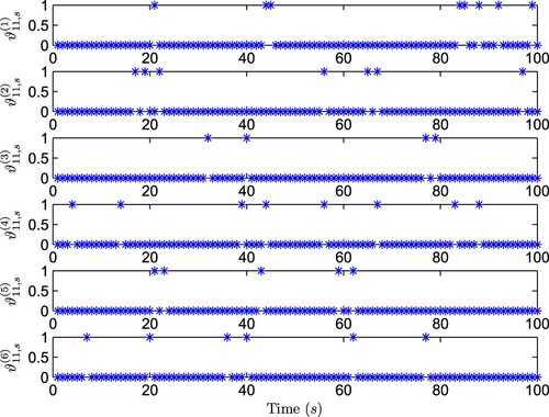$\mathrm{Trace}({\stackrel{`}{\mathrm{{\rm Y}}}}_{i,s|s})$) and the MSE which further verifies the effectiveness of the proposed algorithm and Figure 4 describes the occurrence of bit errors of $y_{11,s}$ in sensor 1, in which the value ‘1’ in the vertical axis indicates that there appears bit error according to (15(15) ${\vartheta }_{i\ell ,s}^{(\varsigma )}=\{\begin{array}{ll}1,& \text{bit error occurs,}\\ 0,& \text{bit error does not occur}.\end{array}$(15) ). It is noted that the crossover probability q given in this simulation is 0.06, which may be smaller in actual transmission cases (e.g. the crossover probability range of ${10}^{-6}$ –${10}^{-2}$ has been considered in Gungor et al. (2010), and it has also been observed in Leung et al. (2015) that for the IEEE 802.15.4 type wireless sensor networks, once the crossover probability reaches 0.1, the receiver modules would not be able to keep the connectivity). The simulation results show that, in spite of the occurrence of bit errors, the designed estimator (27(27) $\begin{array}{rl}{\hat{x}}_{i,s+1|s}& ={\overline{A}}_s{\hat{x}}_{i,s|s}\end{array}$(27) )–(28(28) $\begin{array}{rl}{\hat{x}}_{i,s+1|s+1}& ={\hat{x}}_{i,s+1|s}+{\mathrm{\Im }}_i^{\mathrm{in}}{G}_{i,s+1}(m_i(s+1,y_{i,s+1},N)\\ & -{\overline{C}}_{0,s+1}{\hat{x}}_{i,s+1|s})+K_{i,s+1}\sum _{j\in {\mathbf{N}}_i}{a}_{ji}({\tilde{y}}_{j,s+1}\\ & -{\overline{C}}_{0,s+1}{\hat{x}}_{i,s+1|s})\end{array}$(28) ) has satisfactory fault estimation performance for discrete time-varying systems (1(1) $x_{s+1}=A_s{x}_s+E_s{\omega }_s$(1) ) with binary encoding schemes over a sensor network.

Figure 1. Sensor fault $f_{i,s}$ ($i=1,2,\dots ,5$) and its estimation.

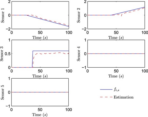
Figure 2. State estimation error of sensor 1.

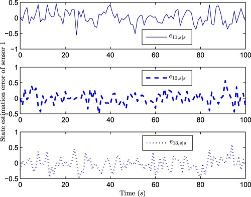
Figure 3. The trace of the minimal upper bound on EE covariance and the MSE of sensor 1.

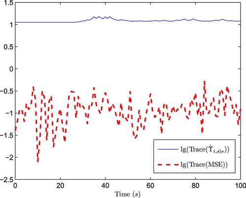
Figure 4. The occurrence of bit error of $y_{11,s}$.

5. Conclusion

This paper has studied the distributed recursive fault estimation problem in binary-coded discrete-time systems based on sensor networks. Sensor faults have been modelled to characterize the fault signal property of second-order difference being zero. The BESs have been adopted in the communication channel from the neighbouring sensors to the local fault estimator, and a random variable with Bernoulli distribution has been used to describe bit errors. To attenuate the influence of bit errors on the fault estimation error, a distributed estimator has been constructed. An upper bound for the estimation error covariance matrix has been computed and then minimized by virtue of designing the proper estimator parameters. Finally, a simulation example has proved the effectiveness and the superiority of the estimation method. For subsequent research directions, we focus on coping with the fault estimation for sensor network systems with model complexities (time delays: Chen et al., 2020, uncertainties: Li & Liang, 2020, multiplicative noises: Wang et al., 2021, energy-bounded noises: Wen et al., 2021, randomly switching topologies: J. Hu et al., 2020, unknown inputs: Zou et al., 2020, time-varying parameters: Hu et al., 2018, state saturations: Shen et al., 2020 and nonlinearities: Mao et al., 2021) and incomplete measurements (channel fadings: L. Liu et al., 2021, quantizations: Zhao et al., 2020, censored measurements: X. Li et al., 2020, outliers: Shen et al., 2021, cyber attacks: Hou et al., 2020 and measurements only from partial nodes: J. Li et al., 2020), respectively.

Disclosure statement

The authors declare that they have no conflict of interest.

Additional information

Funding

This work was supported in part by the National Natural Science Foundation of China under Grants U21A2019, 61873058, 61933007, 62073070, 11902072 and 62103096, the Natural Science Foundation of Heilongjiang Province of China under Grant LH2021F006, the China Postdoctoral Science Foundation under Grants 2017M621242 and 2020T130092, the Fundamental Research Funds for Undergraduate Universities affiliated to Heilongjiang Province of China under Grant XNYXLY202104, the Hainan Province Science and Technology Special Fund under Grant ZDYF2022SHFZ105, the Technology Plan Project of Daqing City of China under Grants zd-2019-17 and zd-2020-26 and the Alexander von Humboldt Foundation of Germany.

References

- Alippi, C., & Galperti, C. (2008). An adaptive system for optimal solar energy harvesting in wireless sensor network nodes. IEEE Transactions on Circuits and Systems-I: Regular Papers, 55(6), 1742–1750. https://doi.org/10.1109/TCSI.2008.922023
- Aysal, T. C., Coates, M., & Rabbat, M. (2007). Distributed average consensus using probabilistic quantization. In 2007 IEEE/SP 14th Workshop on Statistical Signal Processing (pp. 640–644). IEEE
- Battilotti, S., & Mekhail, M. (2019). Distributed estimation for nonlinear systems. Automatica, 107(9), 562–573. https://doi.org/10.1016/j.automatica.2019.06.024
- Caballero-Águila, R., Hermoso-Carazo, A., & Linares-Pérez, J. (2017). New distributed fusion filtering algorithm based on covariances over sensor networks with random packet dropouts. International Journal of Systems Science, 48(9), 1805–1817. https://doi.org/10.1080/00207721.2017.1289568
- Cao, L., Ren, H., Li, H., & Lu, R. (2021). Event-triggered output-feedback control for large-scale systems with unknown hysteresis. IEEE Transactions on Cybernetics, 51(11), 5236–5247. https://doi.org/10.1109/TCYB.2020.2997943
- Chen, H., & Jiang, B. (2020). A review of fault detection and diagnosis for the traction system in high-speed trains. IEEE Transactions on Intelligent Transportation Systems, 21(2), 450–465. https://doi.org/10.1109/TITS.6979
- Chen, Y., Chen, Z., Chen, Z., & Xue, A. (2020). Observer-based passive control of non-homogeneous Markov jump systems with random communication delays. International Journal of Systems Science, 51(6), 1133–1147. https://doi.org/10.1080/00207721.2020.1752844
- Cong, G., Han, F., Li, J., & Dai, D. (2021). Event-triggered distributed filtering for discrete-time systems with integral measurements. Systems Science & Control Engineering, 9(1), 272–282. https://doi.org/10.1080/21642583.2021.1901157
- Ding, D., Wang, Z., Dong, H., & Shu, H. (2012). Distributed H∞ state estimation with stochastic parameters and nonlinearities through sensor networks: The finite-horizon case. Automatica, 48(8), 1575–1585. https://doi.org/10.1016/j.automatica.2012.05.070
- Ding, D., Wang, Z., Ho, D. W. C., & Wei, G. (2017). Distributed recursive filtering for stochastic systems under uniform quantizations and deception attacks through sensor networks. Automatica, 78(1), 231–240. https://doi.org/10.1016/j.automatica.2016.12.026
- Dong, H., Wang, Z., & Gao, H. (2013). Distributed H∞ filtering for a class of Markovian jump nonlinear time-delay systems over lossy sensor networks. IEEE Transactions on Industrial Electronics, 60(10), 4665–4672. https://doi.org/10.1109/TIE.2012.2213553
- Gao, H., Dong, H., Wang, Z., & Han, F. (2020). An event-triggering approach to recursive filtering for complex networks with state saturations and random coupling strengths. IEEE Transactions on Neural Networks and Learning Systems, 31(10), 4279–4289. https://doi.org/10.1109/TNNLS.5962385
- Gao, M., Yang, S., Sheng, L., & Zhou, D. (2019). Fault diagnosis for time-varying systems with multiplicative noises over sensor networks subject to Round-Robin protocol. Neurocomputing, 346(5), 65–72. https://doi.org/10.1016/j.neucom.2018.08.087
- Ge, X., Han, Q.-L., & Wang, Z. (2019a). A dynamic event-triggered transmission scheme for distributed set-membership estimation over wireless sensor networks. IEEE Transactions on Cybernetics, 49(1), 171–183. https://doi.org/10.1109/TCYB.2017.2769722
- Ge, X., Han, Q.-L., & Wang, Z. (2019b). A threshold-parameter-dependent approach to designing distributed event-triggered H∞ consensus filters over sensor networks. IEEE Transactions on Cybernetics, 49(4), 1148–1159. https://doi.org/10.1109/TCYB.6221036
- Geng, H., Liu, H., Ma, L., & Yi, X. (2021). Multi-sensor filtering fusion meets censored measurements under a constrained network environment: Advances, challenges and prospects. International Journal of Systems Science, 52(16), 3410–3436. https://doi.org/10.1080/00207721.2021.2005178
- Gungor, V. C., Liu, B., & Hancke, G. P. (2010). Opportunities and challenges of wireless sensor networks in smart grid. IEEE Transactions on Industrial Electronics, 57(10), 3557–3564. https://doi.org/10.1109/TIE.2009.2039455
- Hou, N., Wang, Z., Ho, D. W. C., & Dong, H. (2020). Robust partial-nodes-based state estimation for complex networks under deception attacks. IEEE Transactions on Cybernetics, 50(6), 2793–2802. https://doi.org/10.1109/TCYB.6221036
- Hu, J., Wang, Z., & Gao, H. (2018). Joint state and fault estimation for time-varying nonlinear systems with randomly occurring faults and sensor saturations. Automatica, 97(7), 150–160. https://doi.org/10.1016/j.automatica.2018.07.027
- Hu, J., Wang, Z., Liu, G.-P., Jia, C., & Williams, J. (2020). Event-triggered recursive state estimation for dynamical networks under randomly switching topologies and multiple missing measurements. Automatica, 115, 108908-1–108908-13. https://doi.org/10.1016/j.automatica.2020.108908
- Hu, S., Yue, D., Han, Q.-L., Xie, X., Chen, X., & Dou, C. (2020). Observer-based event-triggered control for networked linear systems subject to denial-of-service attacks. IEEE Transactions on Cybernetics, 50(5), 1952–1964. https://doi.org/10.1109/TCYB.6221036
- Jia, X.-C. (2021). Resource-efficient and secure distributed state estimation over wireless sensor networks: A survey. International Journal of Systems Science, 52(16), 3368–3389. https://doi.org/10.1080/00207721.2021.1998843
- Leung, H., Seneviratne, C., & Xu, M. (2015). A novel statistical model for distributed estimation in wireless sensor networks. IEEE Transactions on Signal Processing, 63(12), 3154–3164. https://doi.org/10.1109/TSP.2015.2420536
- Li, J., Dong, H., Wang, Z., & Bu, X. (2020). Partial-neurons-based passivity-guaranteed state estimation for neural networks with randomly occurring time-delays. IEEE Transactions on Neural Networks and Learning Systems, 31(9), 3747–3753. https://doi.org/10.1109/TNNLS.5962385
- Li, J., Ma, Y., & Fu, L. (2019). Fault-tolerant passive synchronization for complex dynamical networks with Markovian jump based on sampled-data control. Neurocomputing, 350(6684), 20–32. https://doi.org/10.1016/j.neucom.2019.03.059
- Li, Q., & Liang, J. (2020). Dissipativity of the stochastic Markovian switching CVNNs with randomly occurring uncertainties and general uncertain transition rates. International Journal of Systems Science, 51(6), 1102–1118. https://doi.org/10.1080/00207721.2020.1752418
- Li, X., Han, F., Hou, N., Dong, H., & Liu, H. (2020). Set-membership filtering for piecewise linear systems with censored measurements under Round-Robin protocol. International Journal of Systems Science, 51(9), 1578–1588. https://doi.org/10.1080/00207721.2020.1768453
- Li, X.-J., & Yang, G.-H. (2017). Adaptive fault-tolerant synchronization control of a class of complex dynamical networks with general input distribution matrices and actuator faults. IEEE Transactions on Neural Networks and Learning Systems, 28(3), 559–569. https://doi.org/10.1109/TNNLS.2015.2507183
- Li, Y., Sun, K., & Tong, S. (2019). Observer-based adaptive fuzzy fault-tolerant optimal control for SISO nonlinear systems. IEEE Transactions on Cybernetics, 49(2), 649–661. https://doi.org/10.1109/TCYB.2017.2785801
- Lin, H., & Sun, S. (2019). Globally optimal sequential and distributed fusion state estimation for multi-sensor systems with cross-correlated noises. Automatica, 101(3), 128–137. https://doi.org/10.1016/j.automatica.2018.11.043
- Liu, L., Liu, Y.-J., & Tong, S. (2019). Neural networks-based adaptive finite-time fault-tolerant control for a class of strict-feedback switched nonlinear systems. IEEE Transactions on Cybernetics, 49(7), 2536–2545. https://doi.org/10.1109/TCYB.6221036
- Liu, L., Ma, L., Zhang, J., & Bo, Y. (2021). Distributed non-fragile set-membership filtering for nonlinear systems under fading channels and bias injection attacks. International Journal of Systems Science, 52(6), 1192–1205. https://doi.org/10.1080/00207721.2021.1872118
- Liu, Q., & Wang, Z. (2021). Moving-horizon estimation for linear dynamic networks with binary encoding schemes. IEEE Transactions on Automatic Control, 66(4), 1763–1770. https://doi.org/10.1109/TAC.2020.2996579
- Liu, Q., Wang, Z., He, X., & Zhou, D. H. (2015). Event-based recursive distributed filtering over wireless sensor networks. IEEE Transactions on Automatic Control, 60(9), 2470–2475. https://doi.org/10.1109/TAC.2015.2390554
- Liu, Y., Wang, Z., & Zhou, D. (2021). Resilient actuator fault estimation for discrete-time complex networks: A distributed approach. IEEE Transactions on Automatic Control, 66(9), 4214–4221. https://doi.org/10.1109/TAC.2020.3033710
- Mao, J., Sun, Y., Yi, X., Liu, H., & Ding, D. (2021). Recursive filtering of networked nonlinear systems: A survey. International Journal of Systems Science, 52(6), 1110–1128. https://doi.org/10.1080/00207721.2020.1868615
- Morrow, R. K., & Lehnert, J. S. (1989). Bit-to-bit error dependence in slotted DS/SSMA packet systems with random signature sequences. IEEE Transactions on Communications, 37(10), 1052–1061. https://doi.org/10.1109/26.41160
- Selvaraj, P., Sakthivel, R., & Kwon, O. M. (2018). Synchronization of fractional-order complex dynamical network with random coupling delay, actuator faults and saturation. Nonlinear Dynamics, 94(4), 3101–3116. https://doi.org/10.1007/s11071-018-4516-3
- Shen, B., Wang, Z., Wang, D., & Li, Q. (2020). State-saturated recursive filter design for stochastic time-varying nonlinear complex networks under deception attacks. IEEE Transactions on Neural Networks and Learning Systems, 31(10), 3788–3800. https://doi.org/10.1109/TNNLS.5962385
- Shen, Y., Wang, Z., Shen, B., & Dong, H. (2021). Outlier-resistant recursive filtering for multi-sensor multi-rate networked systems under weighted Try-Once-Discard protocol. IEEE Transactions on Cybernetics, 51(10), 4897–4908. https://doi.org/10.1109/TCYB.2020.3021194
- Song, B., Qi, G., & Xu, L. (2020). A new approach to open-circuit fault diagnosis of MMC sub-module. Systems Science & Control Engineering, 8(1), 119–127. https://doi.org/10.1080/21642583.2020.1731005
- Wang, M., Wang, Z., Dong, H., & Han, Q.-L. (2021). A novel framework for backstepping-based control of discrete-time strict-feedback nonlinear systems with multiplicative noises. IEEE Transactions on Automatic Control, 66(4), 1484–1496. https://doi.org/10.1109/TAC.2020.2995576
- Wang, Z., Wang, L., Liu, S., & Wei, G. (2018). Encoding-decoding-based control and filtering of networked systems: Insights, developments and opportunities. IEEE/CAA Journal of Automatica Sinica, 5(1), 3–18. https://doi.org/10.1109/JAS.2017.7510727
- Wen, P., Hou, N., Shen, Y., Li, J., & Zhang, Y. (2021). Observer-based H∞ PID control for discrete-time systems under hybrid cyber attacks. Systems Science & Control Engineering, 9(1), 232–242. https://doi.org/10.1080/21642583.2021.1895004
- Xu, W., Hu, G., Ho, D. W. C., & Feng, Z. (2020). Distributed secure cooperative control under denial-of-service attacks from multiple adversaries. IEEE Transactions on Cybernetics, 50(8), 3458–3467. https://doi.org/10.1109/TCYB.6221036
- Ye, D., Yang, X., & Su, L. (2017). Fault-tolerant synchronization control for complex dynamical networks with semi-Markov jump topology. Applied Mathematics and Computation, 312(6), 36–48. https://doi.org/10.1016/j.amc.2017.05.008
- Zhang, D., Cai, W., Xie, L., & Wang, Q. (2015). Nonfragile distributed filtering for T-S fuzzy systems in sensor networks. IEEE Transactions on Fuzzy Systems, 23(5), 1883–1890. https://doi.org/10.1109/TFUZZ.2014.2367101
- Zhang, X.-M., Han, Q.-L., & Zhang, B.-L. (2017). An overview and deep investigation on sampled-data-based event-triggered control and filtering for networked systems. IEEE Transactions on Industrial Informatics, 13(1), 4–16. https://doi.org/10.1109/TII.2016.2607150
- Zhao, J. (2018). Dynamic state estimation with model uncertainties using H∞ extended Kalman filter. IEEE Transactions on Power Systems, 33(1), 1099–1100. https://doi.org/10.1109/TPWRS.2017.2688131
- Zhao, Z., Wang, Z., Zou, L., & Guo, J. (2020). Set-membership filtering for time-varying complex networks with uniform quantisations over randomly delayed redundant channels. International Journal of Systems Science, 51(16), 3364–3377. https://doi.org/10.1080/00207721.2020.1814898
- Zhu, Y., Zhang, L., & Zheng, W. (2016). Distributed H∞ filtering for a class of discrete-time Markov jump Lur'e systems with redundant channels. IEEE Transactions on Industrial Electronics, 63(3), 1876–1885. https://doi.org/10.1109/TIE.2015.2499169
- Zou, L., Wang, Z., Hu, J., Liu, Y., & Liu, X. (2021). Communication-protocol-based analysis and synthesis of networked systems: Progress, prospects and challenges. International Journal of Systems Science, 52(14), 3013–3034. https://doi.org/10.1080/00207721.2021.1917721
- Zou, L., Wang, Z., Hu, J., & Zhou, D. H. (2020). Moving horizon estimation with unknown inputs under dynamic quantization effects. IEEE Transactions on Automatic Control, 65(12), 5368–5375. https://doi.org/10.1109/TAC.9