Joint state and fault estimation for nonlinear complex networks with mixed time-delays and uncertain inner coupling: non-fragile recursive method

Abstract

In this paper, the non-fragile joint state and fault estimation problem is investigated for a class of nonlinear time-varying complex networks (NTVCNs) with uncertain inner coupling and mixed time-delays. Compared with the constant inner coupling strength in the existing literature, the inner coupling strength is permitted to vary within certain intervals. A new non-fragile model is adopted to describe the parameter perturbations of the estimator gain matrix which is described by zero-mean multiplicative noises. The attention of this paper is focussed on the design of a locally optimal estimation method, which can estimate both the state and the fault at the same time. Then, by reasonably designing the estimator gain matrix, the minimized upper bound of the state estimation error covariance matrix (SEECM) can be obtained. In addition, the boundedness analysis is taken into account, and a sufficient condition is provided to ensure the boundedness of the upper bound of the SEECM by using the mathematical induction. Lastly, a simulation example is provided to testify the feasibility of the joint state and fault estimation scheme.

Keywords:

• Time-varying complex networks
• joint estimation
• non-fragile recursive method
• mixed time-delays
• uncertain inner coupling

1. Introduction

The complex networks (CNs) with complicated coupling structure have been developed rapidly. From then on, the CNs have been widely used to model a lot of practical systems, such as social network, biological network, and electrical power grids. However, it is almost impossible to obtain all node states in practical applications due to the technique and cost constraints. Consequently, it is significant to estimate the states of CNs by resorting to valid state estimation strategy based on the accessible measurement output (Hou et al., 2022; Hu et al., 2021; Shen et al., 2020, 2022; Zou, Wang, Han, et al., 2021). In recent years, the design of state estimation strategy for CNs has received a great deal of research attention (Chen et al., 2021; Duan et al., 2020; Li et al., 2021; Liu, Wang, Liu, et al., 2021; Tan et al., 2021). Specifically, the variance-constrained recursive state estimation (VCRSE) problem has been investigated in Liu, Wang, Liu, et al. (2021) for a class of stochastic CNs with disordered packet and round-robin-based communication schedule. In addition, a theoretical analysis is given to ensure that the estimation error is bounded in the minimum mean-square error sense. On the other hand, the fault estimation for CNs has stirred some research attention. For example, a joint state and fault issue has been handled in Liu et al. (2022) for a class of nonlinear time-varying coupling CNs subject to saturated measurements, where a sufficient condition has been presented to clarify the boundedness of the error dynamics.

Generally, the analysis and synthesis of the CNs are based on an underlying assumption that the coupling strengths are modelled by known constants. Nevertheless, the coupling strengths may be fluctuated in practical applications due to the noise disturbances or channel congestion (Dong et al., 2020; Huang et al., 2021; Li & Xu, 2021; Luo et al., 2021; Sheng et al., 2018; Wang et al., 2021). Accordingly, some researchers have dedicated to concerning on the CNs with uncertain coupling parameters. For example, in the framework of Kalman-like state estimation, the VCRSE methods have been developed in Gao et al. (2021) and Jia et al. (2020) for nonlinear uncertain coupling CNs, where the bounded coupling parameters have been employed to describe the uncertain coupling perturbations. In addition, Jia et al. (2020) has also introduced a random sequence with known statistical characteristics to embody the random uncertain topologies. Different with the descriptions mentioned above, Wang (2019) has adopted an unknown parameter described by norm bounded uncertainty to model inner coupling parameter perturbation. More generally, the inner coupling matrix may vary in a given interval (Hu et al., 2020). Specifically, the VCRSE strategy has been proposed for a class of CNs with uncertain inner coupling structure and a sufficient condition is given to ensure that the error dynamic is mean-square exponentially bounded.

On another frontier of research, the time-delays have gained the tremendous research interest (Gao et al., 2020; Geng et al., 2021; Ju et al., 2021; Li et al., 2022, 2019; Liu et al., 2020; Ma et al., 2019; Mao et al., 2021; Peng et al., 2018; Shen et al., 2017; Zhang et al., 2017; Zou et al., 2017; Zou, Wang, Hu, et al., 2021), which may give rise to the divergence or oscillation of the networked systems. As everyone knows, the common time-delays mainly include constant time-delays, infinite distributed time-delays, time-varying delays, and so on. Obviously, the analysis and design of state estimation strategy for delayed CNs are more complicated than the delay-free case. Recently, the delay-dependent state estimation issues for CNs have been widely discussed and investigated. For example, a partial-node-based state estimation method against intermittent measurement outliers has been developed in Zou et al. (2022) for a class of delayed CNs, where a sufficient principle regarding the exponentially ultimate boundedness of estimation error has been clarified. By considering the measurable partial-node information, Yu et al. (2021) has investigated the state estimation algorithm design problem for a class of CNs subject to time-varying delays and intermittent dynamic event-triggered schedule, where a sufficient condition to guarantee the exponential stability of error dynamics has been provided. In addition, some authors have gradually paid more attention to the problem of state estimation for CNs with mixed delays and some important results have been published, see e.g. Liu, Shen, et al. (2021) and Wang et al. (2016) for more details. However, it should be pointed out that there are relatively few papers to discuss the VCRSE issue for a class of time-varying CNs with mixed time-delays and fault, which motivates us to carry out such an estimation topic.

In view of the previous analyses, the purpose of this paper is devoted to solving joint state and fault estimation problem for nonlinear time-varying CNs (NTVCNs) with mixed time-delays and uncertain inner coupling. The main three difficulties and challenges encountered are emphasized as: (1) How to deal with the mixed time-delays, uncertain coupling and gain perturbation by means of recursive estimation scheme? (2) How to design the desired estimator gain in the sense of minimum mean-square error at each sampling instant? (3) How to evaluate the algorithm performance based on some certain assumption conditions? Compared with the existing literature, the contributions of this paper can be listed as follows: (i) A novel joint state and fault estimator is constructed in the simultaneous presence of uncertain coupling and gain perturbation; (ii) the estimator gain is parameterized for the purpose of minimizing the trace of the upper bound of SEECM; and (iii) a sufficient condition is given to ensure the uniform boundedness of the developed recursive joint estimation strategy.

Notations. The notations used here are standard. ${\mathbb{R}}^n$ denotes the n dimensional Euclidean space. $\mathrm{t}\mathrm{r}\left(X\right)$ means the trace of the matrix X. The notation $X>Y(X\ge Y)$ stands for X−Y is positive definite (positive semi-definite) for symmetric matrices X and Y. I represents the identity matrix with compatible dimension. For a matrix X, $X^T$ and $X^{-1}$ denote the transpose and inverse of the matrix X, respectively. $\mathbb{E}\{\cdot \}$ stands for the expectation of a random variable. $\Vert \cdot \Vert$ is the Euclidean norm in ${\mathbb{R}}^n$.

2. Problem formulation and preliminaries

Consider the following NTVCNs with N network nodes: (1) $\begin{array}{rl}{\tilde{x}}_{i,h+1}& ={\tilde{A}}_{i,h}{\tilde{x}}_{i,h}+\tilde{g}\left({\tilde{x}}_{i,h}\right)+\sum _{j=1}^N{\omega }_{ij}\tilde{\mathrm{\Gamma }}{\tilde{x}}_{j,h-{\tau }_1}\\ & +{\tilde{F}}_{i,h}{f}_{i,h}+{\tilde{D}}_{i,h}{w}_{i,h},\end{array}$(1) (2) $\begin{array}{rl}{\tilde{y}}_{i,h}& ={\alpha }_{i,h}{\tilde{H}}_{i,h}{\tilde{x}}_{i,h}+(1-{\alpha }_{i,h}){\tilde{H}}_{i,h}{\tilde{x}}_{i,h-{\tau }_2}\\ & +{\nu }_{i,h},\end{array}$(2) where ${\tilde{x}}_{i,h}\in {\mathbb{R}}^n$ with initial state ${\tilde{x}}_{i,0}$ denotes the state vector of the ith node at step h, ${\tilde{y}}_{i,h}\in {\mathbb{R}}^m$ denotes measurement vector of the ith node, and $f_{i,h}\in {\mathbb{R}}^f$ is the fault vector of the ith node satisfying $f_{i,h+1}=f_{i,h}$. $\tilde{g}\left({\tilde{x}}_{i,h}\right)$ is a known nonlinear function. ${\tau }_1$ and ${\tau }_2$ represent the known constant time-delays. $W=[{\omega }_{ij}{]}_{N\times N}$ is the coupling configuration matrix. The process noise $w_{i,h}$ and the measurement noise ${\nu }_{i,h}$ are assumed to be mutually independent zero-mean white Gaussian noises whose covariance matrices are $Q_{i,h}>0$ and $R_{i,h}>0$, respectively. ${\tilde{A}}_{i,h}$, ${\tilde{D}}_{i,h}$ and ${\tilde{H}}_{i,h}$ are known matrices with appropriate dimensions. The random variable ${\alpha }_{i,h}$ obeying the Bernoulli distribution satisfies $\begin{array}{rl}\mathrm{P}\mathrm{r}\mathrm{o}\mathrm{b}\{{\alpha }_{i,h}=1\}& =\mathbb{E}\left\{{\alpha }_{i,h}\right\}={\overline{\alpha }}_{i,h},\\ \mathrm{P}\mathrm{r}\mathrm{o}\mathrm{b}\{{\alpha }_{i,h}=0\}& =1-{\overline{\alpha }}_{i,h}.\end{array}$ In (1(1) $\begin{array}{rl}{\tilde{x}}_{i,h+1}& ={\tilde{A}}_{i,h}{\tilde{x}}_{i,h}+\tilde{g}\left({\tilde{x}}_{i,h}\right)+\sum _{j=1}^N{\omega }_{ij}\tilde{\mathrm{\Gamma }}{\tilde{x}}_{j,h-{\tau }_1}\\ & +{\tilde{F}}_{i,h}{f}_{i,h}+{\tilde{D}}_{i,h}{w}_{i,h},\end{array}$(1) ), $\tilde{\mathrm{\Gamma }}=\mathrm{d}\mathrm{i}\mathrm{a}\mathrm{g}\{{\tilde{\gamma }}_1,{\tilde{\gamma }}_2,\dots ,{\tilde{\gamma }}_n\}$ is the inner-couplingmatrix. The following case that the unknown coupling strength ${\tilde{\gamma }}_i(i=1,2,\dots ,N)$ belongs to a certain range$[{\underset{\_}{\gamma }}_i,{\overline{\gamma }}_i]$ is considered, where ${\underset{\_}{\gamma }}_i$ and ${\overline{\gamma }}_i$ are known with ${\underset{\_}{\gamma }}_i<{\overline{\gamma }}_i$. Let (3) $\begin{array}{rl}{\tilde{\mathrm{\Gamma }}}_1& =\mathrm{d}\mathrm{i}\mathrm{a}\mathrm{g}\{\frac{{\underset{\_}{\gamma }}_1+{\overline{\gamma }}_1}{2},\frac{{\underset{\_}{\gamma }}_2+{\overline{\gamma }}_2}{2},\dots ,\frac{{\underset{\_}{\gamma }}_N+{\overline{\gamma }}_N}{2}\},\end{array}$(3) (4) $\begin{array}{rl}{\tilde{\mathrm{\Gamma }}}_2& =\mathrm{d}\mathrm{i}\mathrm{a}\mathrm{g}\{\frac{{\underset{\_}{\gamma }}_1-{\overline{\gamma }}_1}{2},\frac{{\underset{\_}{\gamma }}_2-{\overline{\gamma }}_2}{2},\dots ,\frac{{\underset{\_}{\gamma }}_N-{\overline{\gamma }}_N}{2}\},\end{array}$(4) then $\tilde{\mathrm{\Gamma }}$ can be written as $\tilde{\mathrm{\Gamma }}={\tilde{\mathrm{\Gamma }}}_1+\overrightarrow{\mathrm{\Gamma }}$ with $\overrightarrow{\mathrm{\Gamma }}\in [-{\tilde{\mathrm{\Gamma }}}_2,{\tilde{\mathrm{\Gamma }}}_2]$. Whereafter $\tilde{\mathrm{\Gamma }}$ can be rewritten as (5) $\tilde{\mathrm{\Gamma }}={\tilde{\mathrm{\Gamma }}}_1+F{\tilde{\mathrm{\Gamma }}}_2,F{F}^T\le I$(5) where $F=\overrightarrow{\mathrm{\Gamma }}{\tilde{\mathrm{\Gamma }}}_2^{-1}$.

Setting $x_{i,h}=[{\tilde{x}}_{i,h}^T{f}_{i,h}^T{]}^T$, we can get (6) $\begin{array}{rl}{x}_{i,h+1}& =A_{i,h}{x}_{i,h}+g\left(x_{i,h}\right)+\sum _{j=1}^N{\omega }_{ij}\mathrm{\Gamma }{x}_{j,h-{\tau }_1}\\ & +D_{i,h}{w}_{i,h},\end{array}$(6) (7) $\begin{array}{rl}{y}_{i,h}& ={\alpha }_{i,h}{H}_{i,h}{x}_{i,h}+(1-{\alpha }_{i,h})H_{i,h}{x}_{i,h-{\tau }_2}\\ & +{\nu }_{i,h},\end{array}$(7) where $\begin{array}{rl}{A}_{i,h}& =\left[\begin{array}{cc}{\tilde{A}}_{i,h}& {\tilde{F}}_{i,h}\\ 0& I\end{array}\right],\mathrm{\Gamma }=\left[\begin{array}{cc}\tilde{\mathrm{\Gamma }}& 0\\ 0& 0\end{array}\right],\\ g\left(x_{i,h}\right)& =\left[\begin{array}{c}\tilde{g}\left({\tilde{x}}_{i,h}\right)\\ 0\end{array}\right],D_{i,h}=\left[\begin{array}{c}{\tilde{D}}_{i,h}\\ 0\end{array}\right],\\ H_{i,h}& =\left[\begin{array}{cc}{\tilde{H}}_{i,h}& 0\end{array}\right],y_{i,h}={\tilde{y}}_{i,h}.\end{array}$

Assumption 2.1

The nonlinear function $\tilde{g}\left({\tilde{x}}_{i,h}\right)$ is known and satisfies the following Lipschitz condition: $\Vert \tilde{g}\left(\varsigma \right)-\tilde{g}\left(\varphi \right)\Vert \le l\Vert (\varsigma -\varphi )\Vert ,$ where l is a known constant.

For the augmented NTVCNs, we construct the joint estimator as follows: (8) $\begin{array}{rl}{\hat{x}}_{i,h+1|h}& =A_{i,h}{\hat{x}}_{i,h|h}+g\left({\hat{x}}_{i,h|h}\right)\\ & +\sum _{j=1}^N{\omega }_{ij}{\mathrm{\Gamma }}_1{\hat{x}}_{j,h-{\tau }_1|h-{\tau }_1},\end{array}$(8) (9) $\begin{array}{rl}{\hat{x}}_{i,h+1|h+1}& ={\hat{x}}_{i,h+1|h}+(K_{i,h+1}+{\delta }_{i,h+1}{\overline{K}}_{i,h+1})\\ & \times [y_{i,h+1}-{\overline{\alpha }}_{i,h+1}{H}_{i,h+1}{\hat{x}}_{i,h+1|h}\\ & -(1-{\overline{\alpha }}_{i,h+1})H_{i,h+1}{\hat{x}}_{i,h-{\tau }_2+1|h-{\tau }_2+1}],\end{array}$(9) where ${\mathrm{\Gamma }}_1=\mathrm{d}\mathrm{i}\mathrm{a}\mathrm{g}\{{\tilde{\mathrm{\Gamma }}}_1,0\}$, ${\hat{x}}_{i,h+1|h}$ and ${\hat{x}}_{i,h+1|h+1}$ denote one-step prediction and state estimation, respectively. $K_{i,h+1}$ is the estimator gain to be designed at time h + 1. ${\overline{K}}_{i,h+1}$ is a known matrix to describe the gain perturbation case. ${\delta }_{i,h+1}\in \mathbb{R}$ is a multiplicative noise satisfying $\mathbb{E}\left\{{\delta }_{i,h+1}\right\}=0$ and $\mathbb{E}\left\{{\delta }_{i,h+1}^2\right\}=1$. Without loss of generality, assume that ${\tilde{x}}_{i,0}$, $w_{i,h}$, ${\nu }_{i,h}$ and ${\delta }_{i,h}$ are mutually independent.

Remark 2.1

In recent years, the delay-dependentKalman-like state estimation problem has been discussed and investigated increasingly. More generally, the mixed time-delays (constant delay and random occurrence delay) have been addressed in this paper. Obviously, the information including the constant delay and random occurrence delay is utilized to construct the joint state estimator (8(8) $\begin{array}{rl}{\hat{x}}_{i,h+1|h}& =A_{i,h}{\hat{x}}_{i,h|h}+g\left({\hat{x}}_{i,h|h}\right)\\ & +\sum _{j=1}^N{\omega }_{ij}{\mathrm{\Gamma }}_1{\hat{x}}_{j,h-{\tau }_1|h-{\tau }_1},\end{array}$(8) )–(9(9) $\begin{array}{rl}{\hat{x}}_{i,h+1|h+1}& ={\hat{x}}_{i,h+1|h}+(K_{i,h+1}+{\delta }_{i,h+1}{\overline{K}}_{i,h+1})\\ & \times [y_{i,h+1}-{\overline{\alpha }}_{i,h+1}{H}_{i,h+1}{\hat{x}}_{i,h+1|h}\\ & -(1-{\overline{\alpha }}_{i,h+1})H_{i,h+1}{\hat{x}}_{i,h-{\tau }_2+1|h-{\tau }_2+1}],\end{array}$(9) ), which may deteriorate the joint estimation accuracy without effective handling manner. This paper makes great effort to develop the joint state and fault estimation method against mixed time-delays based on the Kalman-like estimation strategy.

For node i, the one-step prediction error and the estimation error are defined as follows: (10) $\begin{array}{rl}{e}_{i,h+1|h}& =x_{i,h+1}-{\hat{x}}_{i,h+1|h},\end{array}$(10) (11) $\begin{array}{rl}{e}_{i,h+1|h+1}& =x_{i,h+1}-{\hat{x}}_{i,h+1|h+1},\end{array}$(11) and the corresponding covariance matrices are defined as: (12) $\begin{array}{rl}{P}_{i,h+1|h}& =\mathbb{E}\left\{e_{i,h+1|h}{e}_{i,h+1|h}^T\right\},\end{array}$(12) (13) $\begin{array}{rl}{P}_{i,h+1|h+1}& =\mathbb{E}\left\{e_{i,h+1|h+1}{e}_{i,h+1|h+1}^T\right\}.\end{array}$(13) According to (6(6) $\begin{array}{rl}{x}_{i,h+1}& =A_{i,h}{x}_{i,h}+g\left(x_{i,h}\right)+\sum _{j=1}^N{\omega }_{ij}\mathrm{\Gamma }{x}_{j,h-{\tau }_1}\\ & +D_{i,h}{w}_{i,h},\end{array}$(6) ) and (8(8) $\begin{array}{rl}{\hat{x}}_{i,h+1|h}& =A_{i,h}{\hat{x}}_{i,h|h}+g\left({\hat{x}}_{i,h|h}\right)\\ & +\sum _{j=1}^N{\omega }_{ij}{\mathrm{\Gamma }}_1{\hat{x}}_{j,h-{\tau }_1|h-{\tau }_1},\end{array}$(8) ), the one-step prediction error can be given as: (14) $\begin{array}{rl}& e_{i,h+1|h}\\ & =A_{i,h}{e}_{i,h|h}+g\left(x_{i,h}\right)-g\left({\hat{x}}_{i,h|h}\right)+\sum _{j=1}^N{\omega }_{ij}\overline{\mathrm{\Gamma }}{x}_{j,h-{\tau }_1}\\ & +\sum _{j=1}^N{\omega }_{ij}{\mathrm{\Gamma }}_1{e}_{j,h-{\tau }_1|h-{\tau }_1}+D_{i,h}{w}_{i,h},\end{array}$(14) where $\overline{\mathrm{\Gamma }}=\mathrm{d}\mathrm{i}\mathrm{a}\mathrm{g}\{\overrightarrow{\mathrm{\Gamma }},0\}$. Similarly, the estimation error is derived as: (15) $\begin{array}{rl}& e_{i,h+1|h+1}\\ & =[I-{\overline{\alpha }}_{i,h+1}(K_{i,h+1}+{\delta }_{i,h+1}{\overline{K}}_{i,h+1}\left)H_{i,h+1}\right]e_{i,h+1|h}\\ & -{\tilde{\alpha }}_{i,h+1}(K_{i,h+1}+{\delta }_{i,h+1}{\overline{K}}_{i,h+1})H_{i,h+1}\\ & \times (x_{i,h+1}-x_{i,h-{\tau }_2+1})-(1-{\overline{\alpha }}_{i,h+1})\\ & \times (K_{i,h+1}+{\delta }_{i,h+1}{\overline{K}}_{i,h+1})H_{i,h+1}{e}_{i,h-{\tau }_2+1|h-{\tau }_2+1}\\ & -(K_{i,h+1}+{\delta }_{i,h+1}{\overline{K}}_{i,h+1}){\nu }_{i,h+1},\end{array}$(15) where ${\tilde{\alpha }}_{i,h+1}={\alpha }_{i,h+1}-{\overline{\alpha }}_{i,h+1}$.

3. Main results

In this section, the covariance matrices about the one-step prediction error and state estimation error will be calculated and the upper bound of the SEECM will be acquired. Then, the explicit form of the estimator gain will be obtained by solving two Riccati-like difference equations and the upper bound of SEECM is minimized at each sampling moment based on the parameterized gain matrix. To accomplish this section, we introduce the following lemma, which will be very important in the derivations.

Lemma 3.1

Jia et al., 2020

For two real vectors x and y with identical dimensions, the following inequality $x{y}^T+y{x}^T\le ϵx{x}^T+{ϵ}^{-1}y{y}^T$ holds, where $ϵ>0$ is a scalar.

According to the covariance definition, $P_{i,h+1|h}$ and $P_{i,h+1|h+1}$ are presented in the following lemma.

Lemma 3.2

The recursions of the covariance matrices of the one-step prediction error and state estimation error are given by (16) $\begin{array}{rl}{P}_{i,h+1|h}& =A_{i,h}{P}_{i,h|h}{A}_{i,h}^T+\mathbb{E}\{[g\left(x_{i,h}\right)-g\left({\hat{x}}_{i,h|h}\right)]\\ & \times {[g\left(x_{i,h}\right)-g\left({\hat{x}}_{i,h|kh}\right)]}^T\}+\sum _{j=1}^N\sum _{l=1}^N{\omega }_{ij}{\omega }_{il}\overline{\mathrm{\Gamma }}\\ & \times \mathbb{E}\left\{x_{j,h-{\tau }_1}{x}_{l,h-{\tau }_1}^T\right\}{\overline{\mathrm{\Gamma }}}^T+\sum _{j=1}^N\sum _{l=1}^N{\omega }_{ij}{\omega }_{il}{\mathrm{\Gamma }}_1\\ & \times \mathbb{E}\left\{e_{j,h-{\tau }_1|h-{\tau }_1}{e}_{l,h-{\tau }_1|h-{\tau }_1}^T\right\}{\mathrm{\Gamma }}_1^T+D_{i,h}{Q}_{i,h}{D}_{i,h}^T\\ & +\sum _{m=1}^6(Y_m+Y_m^T)\end{array}$(16) and (17) $\begin{array}{rl}& P_{i,h+1|h+1}\\ & =(I-{\overline{\alpha }}_{i,h+1}{K}_{i,h+1}{H}_{i,h+1})P_{i,h+1|h}(I-{\overline{\alpha }}_{i,h+1}{K}_{i,h+1}\\ & \times H_{i,h+1}{)}^T+{\overline{\alpha }}_{i,h+1}^2{\overline{K}}_{i,h+1}{H}_{i,h+1}{P}_{i,h+1|h}{H}_{i,h+1}^T{\overline{K}}_{i,h+1}^T\\ & +{\overline{\alpha }}_{i,h+1}(1-{\overline{\alpha }}_{i,h+1})K_{i,h+1}{H}_{i,h+1}\mathbb{E}\{x_{i,h+1}{x}_{i,h+1}^T\\ & +x_{i,h-{\tau }_2+1}{x}_{i,h-{\tau }_2+1}^T\left\}{H}_{i,h+1}^T{K}_{i,h+1}^T+{\overline{\alpha }}_{i,h+1}\right(1-{\overline{\alpha }}_{i,h+1})\\ & \times {\overline{K}}_{i,h+1}{H}_{i,h+1}\mathbb{E}\{x_{i,h+1}{x}_{i,h+1}^T+x_{i,h-{\tau }_2+1}{x}_{i,h-{\tau }_2+1}^T\}\\ & \times H_{i,h+1}^T{\overline{K}}_{i,h+1}^T+(1-{\overline{\alpha }}_{i,h+1}{)}^2[K_{i,h+1}{H}_{i,h+1}\\ & \times P_{i,h-{\tau }_2+1|h-{\tau }_2+1}{H}_{i,h+1}^T{K}_{i,h+1}^T+{\overline{K}}_{i,h+1}{H}_{i,h+1}\\ & \times P_{i,h-{\tau }_2+1|h-{\tau }_2+1}{H}_{i,h+1}^T{\overline{K}}_{i,h+1}^T]+K_{i,h+1}{R}_{i,h+1}{K}_{i,h+1}^T\\ & +{\overline{K}}_{i,h+1}{R}_{i,h+1}{\overline{K}}_{i,h+1}^T+\sum _{m_1=1}^4(Z_{m_1}+Z_{m_1}^T),\end{array}$(17) where $\begin{array}{rl}{Y}_1& =A_{i,h}\mathbb{E}\left\{e_{i,h|h}{[g\left(x_{i,h}\right)-g\left({\hat{x}}_{i,h|h}\right)]}^T\right\},\\ Y_2& =\sum _{j=1}^N{\omega }_{ij}{A}_{i,h}\mathbb{E}\left\{e_{i,h|h}{x}_{j,h-{\tau }_1}^T\right\}{\overline{\mathrm{\Gamma }}}^T,\\ Y_3& =\sum _{j=1}^N{\omega }_{ij}{A}_{i,h}\mathbb{E}\left\{e_{i,h|h}{e}_{j,h-{\tau }_1|h-{\tau }_1}^T\right\}{\mathrm{\Gamma }}_1^T,\\ Y_4& =\sum _{j=1}^N{\omega }_{ij}\mathbb{E}\left\{[g\left(x_{i,h}\right)-g\left({\hat{x}}_{i,h|h}\right)]x_{j,h-{\tau }_1}^T\right\}{\overline{\mathrm{\Gamma }}}^T,\\ Y_5& =\sum _{j=1}^N{\omega }_{ij}\mathbb{E}\left\{[g\left(x_{i,h}\right)-g\left({\hat{x}}_{i,h|h}\right)]e_{j,h-{\tau }_1|k-{\tau }_1}^T\right\}{\mathrm{\Gamma }}_1^T,\\ Y_6& =\sum _{j=1}^N\sum _{l=1}^N{\omega }_{ij}{\omega }_{il}\overline{\mathrm{\Gamma }}\mathbb{E}\left\{x_{j,h-{\tau }_1}{e}_{l,h-{\tau }_1|h-{\tau }_1}^T\right\}{\mathrm{\Gamma }}_1^T,\\ Z_1& =-(1-{\overline{\alpha }}_{i,h+1})[I-{\overline{\alpha }}_{i,h+1}{K}_{i,h+1}{H}_{i,h+1}]\\ & \times \mathbb{E}\left\{e_{i,h+1|h}{e}_{i,h-{\tau }_2+1|h-{\tau }_2+1}^T\right\}{H}_{i,h+1}^T{K}_{i,h+1}^T,\\ Z_2& ={\overline{\alpha }}_{i,h+1}(1-{\overline{\alpha }}_{i,h+1}){\overline{K}}_{i,h+1}{H}_{i,h+1}\\ & \times \mathbb{E}\left\{e_{i,h+1|h}{e}_{i,h-{\tau }_2+1|h-{\tau }_2+1}^T\right\}{H}_{i,h+1}^T{\overline{K}}_{i,h+1}^T,\\ Z_3& =-{\overline{\alpha }}_{i,h+1}(1-{\overline{\alpha }}_{i,h+1})K_{i,h+1}{H}_{i,h+1}\\ & \times \mathbb{E}\left\{x_{i,h+1}{x}_{i,h-{\tau }_2+1}^T\right\}{H}_{i,h+1}^T{K}_{i,h+1}^T,\\ Z_4& =-{\overline{\alpha }}_{i,h+1}(1-{\overline{\alpha }}_{i,h+1}){\overline{K}}_{i,h+1}{H}_{i,h+1}\\ & \times \mathbb{E}\left\{x_{i,h+1}{x}_{i,h-{\tau }_2+1}^T\right\}{H}_{i,h+1}^T{\overline{K}}_{i,h+1}^T.\end{array}$

Proof.

The proof of this lemma is omitted for brevity.

Subsequently, the following theorem gives the upper bound of SEECM and designs the estimator parameter to optimize the obtained upper bound.

Theorem 3.1

For the augmented NTVCNs described by (6(6) $\begin{array}{rl}{x}_{i,h+1}& =A_{i,h}{x}_{i,h}+g\left(x_{i,h}\right)+\sum _{j=1}^N{\omega }_{ij}\mathrm{\Gamma }{x}_{j,h-{\tau }_1}\\ & +D_{i,h}{w}_{i,h},\end{array}$(6) )–(7(7) $\begin{array}{rl}{y}_{i,h}& ={\alpha }_{i,h}{H}_{i,h}{x}_{i,h}+(1-{\alpha }_{i,h})H_{i,h}{x}_{i,h-{\tau }_2}\\ & +{\nu }_{i,h},\end{array}$(7) ) and joint estimator designed by (8(8) $\begin{array}{rl}{\hat{x}}_{i,h+1|h}& =A_{i,h}{\hat{x}}_{i,h|h}+g\left({\hat{x}}_{i,h|h}\right)\\ & +\sum _{j=1}^N{\omega }_{ij}{\mathrm{\Gamma }}_1{\hat{x}}_{j,h-{\tau }_1|h-{\tau }_1},\end{array}$(8) )–(9(9) $\begin{array}{rl}{\hat{x}}_{i,h+1|h+1}& ={\hat{x}}_{i,h+1|h}+(K_{i,h+1}+{\delta }_{i,h+1}{\overline{K}}_{i,h+1})\\ & \times [y_{i,h+1}-{\overline{\alpha }}_{i,h+1}{H}_{i,h+1}{\hat{x}}_{i,h+1|h}\\ & -(1-{\overline{\alpha }}_{i,h+1})H_{i,h+1}{\hat{x}}_{i,h-{\tau }_2+1|h-{\tau }_2+1}],\end{array}$(9) ), let ${ϵ}_i>0(i=1,\dots ,13)$ be known scalars. Under the initial condition $0<P_{i,0|0}\le {\mathrm{\Sigma }}_{i,0|0}$, if the following two matrix equations (18) $\begin{array}{rl}& {\mathrm{\Sigma }}_{i,h+1|h}\\ & ={\theta }_1{A}_{i,h}{\mathrm{\Sigma }}_{i,h|h}{A}_{i,h}^T+{\theta }_2{l}^2\mathrm{t}\mathrm{r}\left\{{\mathrm{\Sigma }}_{i,h|h}\right\}I+{\theta }_3{\omega }_i\sum _{j=1}^N{\omega }_{ij}\\ & \times \mathrm{t}\mathrm{r}\left\{{\mathrm{\Gamma }}_2{\overrightarrow{\mathrm{\Psi }}}_{j,h-{\tau }_1|h-{\tau }_1}{\mathrm{\Gamma }}_2^T\right\}I+D_{i,h}{Q}_{i,h}{D}_{i,h}^T\\ & +{\theta }_4{\omega }_i\sum _{j=1}^N{\omega }_{ij}{\mathrm{\Gamma }}_1{\mathrm{\Sigma }}_{j,h-{\tau }_1|h-{\tau }_1}{\mathrm{\Gamma }}_1^T,\end{array}$(18) (19) $\begin{array}{rl}& {\mathrm{\Sigma }}_{i,h+1|h+1}\\ & =(1+{ϵ}_8)(I-{\overline{\alpha }}_{i,h+1}{K}_{i,h+1}{H}_{i,h+1}){\mathrm{\Sigma }}_{i,h+1|h}\\ & \times {(I-{\overline{\alpha }}_{i,h+1}{K}_{i,h+1}{H}_{i,h+1})}^T+(1+{ϵ}_9){\overline{\alpha }}_{i,h+1}^2\\ & \times {\overline{K}}_{i,h+1}{H}_{i,h+1}{\mathrm{\Sigma }}_{i,h+1|h}{H}_{i,h+1}^T{\overline{K}}_{i,h+1}^T+{\overline{\alpha }}_{i,h+1}\\ & \times (1-{\overline{\alpha }}_{i,h+1})K_{i,h+1}{H}_{i,h+1}\left[\right(1+{ϵ}_{10}){\overrightarrow{\mathrm{\Delta }}}_{i,h+1|h}\\ & +(1+{ϵ}_{10}^{-1}){\overrightarrow{\mathrm{\Xi }}}_{i,h-{\tau }_2+1|h-{\tau }_2+1}]H_{i,h+1}^T{K}_{i,h+1}^T+{\overline{\alpha }}_{i,h+1}\\ & \times (1-{\overline{\alpha }}_{i,h+1}){\overline{K}}_{i,h+1}{H}_{i,h+1}\left[\right(1+{ϵ}_{11}){\overrightarrow{\mathrm{\Delta }}}_{i,h+1|h}\\ & +(1+{ϵ}_{11}^{-1}){\overrightarrow{\mathrm{\Xi }}}_{i,h-{\tau }_2+1|h-{\tau }_2+1}]H_{i,h+1}^T{\overline{K}}_{i,h+1}^T\\ & +(1-{\overline{\alpha }}_{i,h+1}{)}^2[(1+{ϵ}_8^{-1})K_{i,h+1}{H}_{i,h+1}\\ & \times {\mathrm{\Sigma }}_{i,h-{\tau }_2+1|h-{\tau }_2+1}{H}_{i,h+1}^T{K}_{i,h+1}^T+(1+{ϵ}_9^{-1}){\overline{K}}_{i,h+1}\\ & \times H_{i,h+1}{\mathrm{\Sigma }}_{i,h-{\tau }_2+1|h-{\tau }_2+1}{H}_{i,h+1}^T{\overline{K}}_{i,h+1}^T]+K_{i,h+1}\\ & \times R_{i,h+1}{K}_{i,h+1}^T+{\overline{K}}_{i,h+1}{R}_{i,h+1}{\overline{K}}_{i,h+1}^T,\end{array}$(19) where (20) $\begin{array}{rl}& {\omega }_i=\sum _{j=1}^N{\omega }_{ij},{\mathrm{\Gamma }}_2=\mathrm{d}\mathrm{i}\mathrm{a}\mathrm{g}\{{\tilde{\mathrm{\Gamma }}}_2,0\},\\ & {\theta }_1=1+{ϵ}_1+{ϵ}_2+{ϵ}_3,{\theta }_2=1+{ϵ}_1^{-1}+{ϵ}_4+{ϵ}_5,\\ & {\theta }_3=1+{ϵ}_2^{-1}+{ϵ}_4^{-1}+{ϵ}_6,{\theta }_4=1+{ϵ}_3^{-1}+{ϵ}_5^{-1}+{ϵ}_6^{-1},\\ & {\overrightarrow{\mathrm{\Psi }}}_{j,k-{\tau }_1|h-{\tau }_1}=(1+{ϵ}_7){\hat{x}}_{j,h-{\tau }_1|h-{\tau }_1}{\hat{x}}_{j,h-{\tau }_1|h-{\tau }_1}^T\\ & +(1+{ϵ}_7){\mathrm{\Sigma }}_{j,h-{\tau }_1|k-{\tau }_1},\\ & {\overrightarrow{\mathrm{\Delta }}}_{i,h+1|h}=(1+{ϵ}_{12}){\mathrm{\Sigma }}_{i,h+1|h}\\ & +(1+{ϵ}_{12}^{-1}){\hat{x}}_{i,h+1|h}{\hat{x}}_{i,h+1|h}^T,\\ & {\overrightarrow{\mathrm{\Xi }}}_{i,h-{\tau }_2+1|h-{\tau }_2+1}=(1+{ϵ}_{13}^{-1}){\hat{x}}_{i,h-{\tau }_2+1|h-{\tau }_2+1}\\ & \times {\hat{x}}_{i,h-{\tau }_2+1|h-{\tau }_2+1}^T+(1+{ϵ}_{13}){\mathrm{\Sigma }}_{i,h-{\tau }_2+1|h-{\tau }_2+1},\end{array}$(20) have positive-define solutions ${\mathrm{\Sigma }}_{i,h+1|h}$ and ${\mathrm{\Sigma }}_{i,h+1|h+1}$ at each sampling instant, then one has $P_{i,h+1|h+1}\le {\mathrm{\Sigma }}_{i,h+1|h+1}$. In addition, if the estimator parameter is given as follows: (21) $\begin{array}{rl}{K}_{i,h+1}& =(1+{ϵ}_8){\overline{\alpha }}_{i,h+1}{\mathrm{\Sigma }}_{i,h+1|h}{H}_{i,h+1}^T\\ & \times ({\mathrm{\Sigma }}_{i,h+1}^H+R_{i,h+1}{)}^{-1},\end{array}$(21) where $\begin{array}{rl}& {\mathrm{\Sigma }}_{i,h+1}^H\\ & =(1+{ϵ}_8){\overline{\alpha }}_{i,h+1}^2{H}_{i,h+1}{\mathrm{\Sigma }}_{i,h+1|h}{H}_{i,h+1}^T\\ & +{\overline{\alpha }}_{i,h+1}(1-{\overline{\alpha }}_{i,h+1})H_{i,h+1}\left[\right(1+{ϵ}_{10}){\overrightarrow{\mathrm{\Delta }}}_{i,h+1|h}\\ & +(1+{ϵ}_{10}^{-1}){\overrightarrow{\mathrm{\Xi }}}_{i,h-{\tau }_2+1|h-{\tau }_2+1}]H_{i,h+1}^T+(1-{\overline{\alpha }}_{i,h+1}{)}^2\\ & \times (1+{ϵ}_8^{-1})H_{i,h+1}{\mathrm{\Sigma }}_{i,h-{\tau }_2+1|h-{\tau }_2+1}{H}_{i,h+1}^T,\end{array}$ then $\mathrm{t}\mathrm{r}\left({\mathrm{\Sigma }}_{i,h+1|h+1}\right)$ can be minimized at each sampling instant.

Proof.

This theorem is proved by means of the mathematical induction approach. Under the initial condition $0<P_{i,0|0}\le {\mathrm{\Sigma }}_{i,0|0}$, assuming $P_{i,h|h}\le {\mathrm{\Sigma }}_{i,h|h}$, $P_{i,h+1|h+1}\le {\mathrm{\Sigma }}_{i,h+1|h+1}$ will be furthered verified. Firstly, we aim to seek a matrix ${\mathrm{\Sigma }}_{i,h+1|h}$ satisfying $P_{i,h+1|h}\le {\mathrm{\Sigma }}_{i,h+1|h}$. Based on Lemma 3.1, we have (22) $\begin{array}{rl}& Y_1+Y_1^T\\ & \le {ϵ}_1{A}_{i,h}{P}_{i,h|h}{A}_{i,h}^T+{ϵ}_1^{-1}\mathbb{E}\left\{\right[g\left(x_{i,h}\right)-g\left({\hat{x}}_{i,h|h}\right)]\\ & \times {[g\left(x_{i,h}\right)-g\left({\hat{x}}_{i,h|h}\right)]}^T\},\end{array}$(22) (23) $\begin{array}{rl}& Y_2+Y_2^T\\ & \le {ϵ}_2^{-1}\sum _{j=1}^N\sum _{l=1}^N{\omega }_{ij}{\omega }_{il}\overline{\mathrm{\Gamma }}\mathbb{E}\left\{x_{j,h-{\tau }_1}{x}_{l,h-{\tau }_1}^T\right\}{\overline{\mathrm{\Gamma }}}^T\\ & +{ϵ}_2{A}_{i,h}{P}_{i,h|h}{A}_{i,h}^T,\end{array}$(23) (24) $\begin{array}{rl}& Y_3+Y_3^T\\ & \le {ϵ}_3^{-1}\sum _{j=1}^N\sum _{l=1}^N{\omega }_{ij}{\omega }_{il}{\mathrm{\Gamma }}_1\mathbb{E}\left\{e_{j,h-{\tau }_1|h-{\tau }_1}{e}_{l,h-{\tau }_1|h-{\tau }_1}^T\right\}{\mathrm{\Gamma }}_1^T\\ & +{ϵ}_3{A}_{i,h}{P}_{i,h|h}{A}_{i,h}^T,\end{array}$(24) (25) $\begin{array}{rl}& Y_4+Y_4^T\\ & \le {ϵ}_4^{-1}\sum _{j=1}^N\sum _{l=1}^N{\omega }_{ij}{\omega }_{il}\overline{\mathrm{\Gamma }}\mathbb{E}\left\{x_{j,h-{\tau }_1}{x}_{l,h-{\tau }_1}^T\right\}{\overline{\mathrm{\Gamma }}}^T+{ϵ}_4\\ & \times \mathbb{E}\left\{[g\left(x_{i,h}\right)-g\left({\hat{x}}_{i,h|h}\right)]{[g\left(x_{i,h}\right)-g\left({\hat{x}}_{i,h|h}\right)]}^T\right\},\end{array}$(25) (26) $\begin{array}{rl}& Y_5+Y_5^T\\ & \le {ϵ}_5\mathbb{E}\left\{[g\left(x_{i,h}\right)-g\left({\hat{x}}_{i,h|h}\right)]{[g\left(x_{i,h}\right)-g\left({\hat{x}}_{i,h|h}\right)]}^T\right\}\\ & +{ϵ}_5^{-1}\sum _{j=1}^N\sum _{l=1}^N{\omega }_{ij}{\omega }_{il}{\mathrm{\Gamma }}_1\mathbb{E}\left\{e_{j,h-{\tau }_1|h-{\tau }_1}{e}_{l,h-{\tau }_1|h-{\tau }_1}^T\right\}{\mathrm{\Gamma }}_1^T,\end{array}$(26) (27) $\begin{array}{rl}& Y_6+Y_6^T\\ & \le {ϵ}_6\sum _{j=1}^N\sum _{l=1}^N{\omega }_{ij}{\omega }_{il}\overline{\mathrm{\Gamma }}\mathbb{E}\left\{x_{j,h-{\tau }_1}{x}_{l,h-{\tau }_1}^T\right\}{\overline{\mathrm{\Gamma }}}^T+{ϵ}_6^{-1}\sum _{j=1}^N\sum _{l=1}^N\\ & \times {\omega }_{ij}{\omega }_{il}{\mathrm{\Gamma }}_1\mathbb{E}\left\{e_{j,h-{\tau }_1|h-{\tau }_1}{e}_{l,h-{\tau }_1|h-{\tau }_1}^T\right\}{\mathrm{\Gamma }}_1^T.\end{array}$(27) where ${ϵ}_i>0(i=1,2,\dots ,6)$ are known scalars. Substituting (22(22) $\begin{array}{rl}& Y_1+Y_1^T\\ & \le {ϵ}_1{A}_{i,h}{P}_{i,h|h}{A}_{i,h}^T+{ϵ}_1^{-1}\mathbb{E}\left\{\right[g\left(x_{i,h}\right)-g\left({\hat{x}}_{i,h|h}\right)]\\ & \times {[g\left(x_{i,h}\right)-g\left({\hat{x}}_{i,h|h}\right)]}^T\},\end{array}$(22) )–(27(27) $\begin{array}{rl}& Y_6+Y_6^T\\ & \le {ϵ}_6\sum _{j=1}^N\sum _{l=1}^N{\omega }_{ij}{\omega }_{il}\overline{\mathrm{\Gamma }}\mathbb{E}\left\{x_{j,h-{\tau }_1}{x}_{l,h-{\tau }_1}^T\right\}{\overline{\mathrm{\Gamma }}}^T+{ϵ}_6^{-1}\sum _{j=1}^N\sum _{l=1}^N\\ & \times {\omega }_{ij}{\omega }_{il}{\mathrm{\Gamma }}_1\mathbb{E}\left\{e_{j,h-{\tau }_1|h-{\tau }_1}{e}_{l,h-{\tau }_1|h-{\tau }_1}^T\right\}{\mathrm{\Gamma }}_1^T.\end{array}$(27) ) into (16(16) $\begin{array}{rl}{P}_{i,h+1|h}& =A_{i,h}{P}_{i,h|h}{A}_{i,h}^T+\mathbb{E}\{[g\left(x_{i,h}\right)-g\left({\hat{x}}_{i,h|h}\right)]\\ & \times {[g\left(x_{i,h}\right)-g\left({\hat{x}}_{i,h|kh}\right)]}^T\}+\sum _{j=1}^N\sum _{l=1}^N{\omega }_{ij}{\omega }_{il}\overline{\mathrm{\Gamma }}\\ & \times \mathbb{E}\left\{x_{j,h-{\tau }_1}{x}_{l,h-{\tau }_1}^T\right\}{\overline{\mathrm{\Gamma }}}^T+\sum _{j=1}^N\sum _{l=1}^N{\omega }_{ij}{\omega }_{il}{\mathrm{\Gamma }}_1\\ & \times \mathbb{E}\left\{e_{j,h-{\tau }_1|h-{\tau }_1}{e}_{l,h-{\tau }_1|h-{\tau }_1}^T\right\}{\mathrm{\Gamma }}_1^T+D_{i,h}{Q}_{i,h}{D}_{i,h}^T\\ & +\sum _{m=1}^6(Y_m+Y_m^T)\end{array}$(16) ) leads to (28) $\begin{array}{rl}& P_{i,h+1|h}\\ & \le {\theta }_1{A}_{i,h}{P}_{i,h|h}{A}_{i,h}^T+{\theta }_3\sum _{j=1}^N\sum _{l=1}^N{\omega }_{ij}{\omega }_{il}\overline{\mathrm{\Gamma }}\mathbb{E}\left\{x_{j,h-{\tau }_1}{x}_{l,h-{\tau }_1}^T\right\}\\ & \times {\overline{\mathrm{\Gamma }}}^T+D_{i,h}{Q}_{i,h}{D}_{i,h}^T+{\theta }_2\mathbb{E}\{[g\left(x_{i,h}\right)-g\left({\hat{x}}_{i,h|h}\right)]\\ & \times {[g\left(x_{i,h}\right)-g\left({\hat{x}}_{i,h|h}\right)]}^T\}+{\theta }_4\sum _{j=1}^N\sum _{l=1}^N{\omega }_{ij}{\omega }_{il}\\ & \times {\mathrm{\Gamma }}_1\mathbb{E}\left\{e_{j,h-{\tau }_1|h-{\tau }_1}{e}_{l,h-{\tau }_1|h-{\tau }_1}^T\right\}{\mathrm{\Gamma }}_1^T,\end{array}$(28) where ${\theta }_1$, ${\theta }_2$, ${\theta }_3$, and ${\theta }_4$ are defined in (20(20) $\begin{array}{rl}& {\omega }_i=\sum _{j=1}^N{\omega }_{ij},{\mathrm{\Gamma }}_2=\mathrm{d}\mathrm{i}\mathrm{a}\mathrm{g}\{{\tilde{\mathrm{\Gamma }}}_2,0\},\\ & {\theta }_1=1+{ϵ}_1+{ϵ}_2+{ϵ}_3,{\theta }_2=1+{ϵ}_1^{-1}+{ϵ}_4+{ϵ}_5,\\ & {\theta }_3=1+{ϵ}_2^{-1}+{ϵ}_4^{-1}+{ϵ}_6,{\theta }_4=1+{ϵ}_3^{-1}+{ϵ}_5^{-1}+{ϵ}_6^{-1},\\ & {\overrightarrow{\mathrm{\Psi }}}_{j,k-{\tau }_1|h-{\tau }_1}=(1+{ϵ}_7){\hat{x}}_{j,h-{\tau }_1|h-{\tau }_1}{\hat{x}}_{j,h-{\tau }_1|h-{\tau }_1}^T\\ & +(1+{ϵ}_7){\mathrm{\Sigma }}_{j,h-{\tau }_1|k-{\tau }_1},\\ & {\overrightarrow{\mathrm{\Delta }}}_{i,h+1|h}=(1+{ϵ}_{12}){\mathrm{\Sigma }}_{i,h+1|h}\\ & +(1+{ϵ}_{12}^{-1}){\hat{x}}_{i,h+1|h}{\hat{x}}_{i,h+1|h}^T,\\ & {\overrightarrow{\mathrm{\Xi }}}_{i,h-{\tau }_2+1|h-{\tau }_2+1}=(1+{ϵ}_{13}^{-1}){\hat{x}}_{i,h-{\tau }_2+1|h-{\tau }_2+1}\\ & \times {\hat{x}}_{i,h-{\tau }_2+1|h-{\tau }_2+1}^T+(1+{ϵ}_{13}){\mathrm{\Sigma }}_{i,h-{\tau }_2+1|h-{\tau }_2+1},\end{array}$(20) ). Utilizing Lemma 3.1 yields (29) $\begin{array}{rl}& \mathbb{E}\left\{x_{j,h-{\tau }_1}{x}_{j,h-{\tau }_1}^T\right\}\\ & \le (1+{ϵ}_7)P_{j,h-{\tau }_1|h-{\tau }_1}+(1+{ϵ}_7^{-1})\\ & \times {\hat{x}}_{j,h-{\tau }_1|h-{\tau }_1}{\hat{x}}_{j,h-{\tau }_1|h-{\tau }_1}^T\\ & :={\mathrm{\Psi }}_{j,h-{\tau }_1|h-{\tau }_1},\end{array}$(29) where ${ϵ}_7$ is a positive scalars. Next, let us calculate the second term in (28(28) $\begin{array}{rl}& P_{i,h+1|h}\\ & \le {\theta }_1{A}_{i,h}{P}_{i,h|h}{A}_{i,h}^T+{\theta }_3\sum _{j=1}^N\sum _{l=1}^N{\omega }_{ij}{\omega }_{il}\overline{\mathrm{\Gamma }}\mathbb{E}\left\{x_{j,h-{\tau }_1}{x}_{l,h-{\tau }_1}^T\right\}\\ & \times {\overline{\mathrm{\Gamma }}}^T+D_{i,h}{Q}_{i,h}{D}_{i,h}^T+{\theta }_2\mathbb{E}\{[g\left(x_{i,h}\right)-g\left({\hat{x}}_{i,h|h}\right)]\\ & \times {[g\left(x_{i,h}\right)-g\left({\hat{x}}_{i,h|h}\right)]}^T\}+{\theta }_4\sum _{j=1}^N\sum _{l=1}^N{\omega }_{ij}{\omega }_{il}\\ & \times {\mathrm{\Gamma }}_1\mathbb{E}\left\{e_{j,h-{\tau }_1|h-{\tau }_1}{e}_{l,h-{\tau }_1|h-{\tau }_1}^T\right\}{\mathrm{\Gamma }}_1^T,\end{array}$(28) ) (30) $\begin{array}{rl}& \sum _{j=1}^N\sum _{l=1}^N{\omega }_{ij}{\omega }_{il}\overline{\mathrm{\Gamma }}\mathbb{E}\left\{x_{j,h-{\tau }_1}{x}_{l,h-{\tau }_1}^T\right\}{\overline{\mathrm{\Gamma }}}^T\\ & \le \frac{1}{2}\sum _{j=1}^N\sum _{l=1}^N{\omega }_{ij}{\omega }_{il}\overline{\mathrm{\Gamma }}\mathbb{E}\{x_{j,h-{\tau }_1}{x}_{j,h-{\tau }_1}^T+x_{l,h-{\tau }_1}{x}_{l,h-{\tau }_1}^T\}{\overline{\mathrm{\Gamma }}}^T\\ & ={\omega }_i\sum _{j=1}^N{\omega }_{ij}\overline{\mathrm{\Gamma }}\mathbb{E}\left\{x_{j,h-{\tau }_1}{x}_{j,h-{\tau }_1}^T\right\}{\overline{\mathrm{\Gamma }}}^T\\ & \le {\omega }_i\sum _{j=1}^N{\omega }_{ij}\mathrm{t}\mathrm{r}\left\{{\mathrm{\Gamma }}_2{\mathrm{\Psi }}_{j,h-{\tau }_1|h-{\tau }_1}{\mathrm{\Gamma }}_2^T\right\}I,\end{array}$(30) where ${\omega }_i=\sum _{j=1}^N{\omega }_{ij}$ and ${\mathrm{\Gamma }}_2=\mathrm{d}\mathrm{i}\mathrm{a}\mathrm{g}\{{\tilde{\mathrm{\Gamma }}}_2,0\}$. Then, we deal with the fourth term in (28(28) $\begin{array}{rl}& P_{i,h+1|h}\\ & \le {\theta }_1{A}_{i,h}{P}_{i,h|h}{A}_{i,h}^T+{\theta }_3\sum _{j=1}^N\sum _{l=1}^N{\omega }_{ij}{\omega }_{il}\overline{\mathrm{\Gamma }}\mathbb{E}\left\{x_{j,h-{\tau }_1}{x}_{l,h-{\tau }_1}^T\right\}\\ & \times {\overline{\mathrm{\Gamma }}}^T+D_{i,h}{Q}_{i,h}{D}_{i,h}^T+{\theta }_2\mathbb{E}\{[g\left(x_{i,h}\right)-g\left({\hat{x}}_{i,h|h}\right)]\\ & \times {[g\left(x_{i,h}\right)-g\left({\hat{x}}_{i,h|h}\right)]}^T\}+{\theta }_4\sum _{j=1}^N\sum _{l=1}^N{\omega }_{ij}{\omega }_{il}\\ & \times {\mathrm{\Gamma }}_1\mathbb{E}\left\{e_{j,h-{\tau }_1|h-{\tau }_1}{e}_{l,h-{\tau }_1|h-{\tau }_1}^T\right\}{\mathrm{\Gamma }}_1^T,\end{array}$(28) ). In view of Assumption 2.1, we obtain (31) $\begin{array}{rl}& \mathbb{E}\left\{[g\left(x_{i,h}\right)-g\left({\hat{x}}_{i,h|h}\right)]{[g\left(x_{i,h}\right)-g\left({\hat{x}}_{i,h|h}\right)]}^T\right\}\\ & \le l^2\mathrm{t}\mathrm{r}\left\{P_{i,h|h}\right\}I.\end{array}$(31) Subsequently, with regard to the fifth term in (28(28) $\begin{array}{rl}& P_{i,h+1|h}\\ & \le {\theta }_1{A}_{i,h}{P}_{i,h|h}{A}_{i,h}^T+{\theta }_3\sum _{j=1}^N\sum _{l=1}^N{\omega }_{ij}{\omega }_{il}\overline{\mathrm{\Gamma }}\mathbb{E}\left\{x_{j,h-{\tau }_1}{x}_{l,h-{\tau }_1}^T\right\}\\ & \times {\overline{\mathrm{\Gamma }}}^T+D_{i,h}{Q}_{i,h}{D}_{i,h}^T+{\theta }_2\mathbb{E}\{[g\left(x_{i,h}\right)-g\left({\hat{x}}_{i,h|h}\right)]\\ & \times {[g\left(x_{i,h}\right)-g\left({\hat{x}}_{i,h|h}\right)]}^T\}+{\theta }_4\sum _{j=1}^N\sum _{l=1}^N{\omega }_{ij}{\omega }_{il}\\ & \times {\mathrm{\Gamma }}_1\mathbb{E}\left\{e_{j,h-{\tau }_1|h-{\tau }_1}{e}_{l,h-{\tau }_1|h-{\tau }_1}^T\right\}{\mathrm{\Gamma }}_1^T,\end{array}$(28) ), we have (32) $\begin{array}{rl}& \sum _{j=1}^N\sum _{l=1}^N{\omega }_{ij}{\omega }_{il}{\mathrm{\Gamma }}_1\mathbb{E}\left\{e_{j,h-{\tau }_1|h-{\tau }_1}{e}_{l,h-{\tau }_1|h-{\tau }_1}^T\right\}{\mathrm{\Gamma }}_1^T\\ & \le \frac{1}{2}\sum _{j=1}^N\sum _{l=1}^N{\omega }_{ij}{\omega }_{il}{\mathrm{\Gamma }}_1\mathbb{E}\{e_{j,h-{\tau }_1|h-{\tau }_1}{e}_{j,h-{\tau }_1|h-{\tau }_1}^T\\ & +e_{l,h-{\tau }_1|h-{\tau }_1}{e}_{l,h-{\tau }_1|h-{\tau }_1}^T\}{\mathrm{\Gamma }}_1^T\\ & ={\omega }_i\sum _{j=1}^N{\omega }_{ij}{\mathrm{\Gamma }}_1{P}_{j,h-{\tau }_1|h-{\tau }_1}{\mathrm{\Gamma }}_1^T,\end{array}$(32) Substituting (29(29) $\begin{array}{rl}& \mathbb{E}\left\{x_{j,h-{\tau }_1}{x}_{j,h-{\tau }_1}^T\right\}\\ & \le (1+{ϵ}_7)P_{j,h-{\tau }_1|h-{\tau }_1}+(1+{ϵ}_7^{-1})\\ & \times {\hat{x}}_{j,h-{\tau }_1|h-{\tau }_1}{\hat{x}}_{j,h-{\tau }_1|h-{\tau }_1}^T\\ & :={\mathrm{\Psi }}_{j,h-{\tau }_1|h-{\tau }_1},\end{array}$(29) )–(32(32) $\begin{array}{rl}& \sum _{j=1}^N\sum _{l=1}^N{\omega }_{ij}{\omega }_{il}{\mathrm{\Gamma }}_1\mathbb{E}\left\{e_{j,h-{\tau }_1|h-{\tau }_1}{e}_{l,h-{\tau }_1|h-{\tau }_1}^T\right\}{\mathrm{\Gamma }}_1^T\\ & \le \frac{1}{2}\sum _{j=1}^N\sum _{l=1}^N{\omega }_{ij}{\omega }_{il}{\mathrm{\Gamma }}_1\mathbb{E}\{e_{j,h-{\tau }_1|h-{\tau }_1}{e}_{j,h-{\tau }_1|h-{\tau }_1}^T\\ & +e_{l,h-{\tau }_1|h-{\tau }_1}{e}_{l,h-{\tau }_1|h-{\tau }_1}^T\}{\mathrm{\Gamma }}_1^T\\ & ={\omega }_i\sum _{j=1}^N{\omega }_{ij}{\mathrm{\Gamma }}_1{P}_{j,h-{\tau }_1|h-{\tau }_1}{\mathrm{\Gamma }}_1^T,\end{array}$(32) ) into (28(28) $\begin{array}{rl}& P_{i,h+1|h}\\ & \le {\theta }_1{A}_{i,h}{P}_{i,h|h}{A}_{i,h}^T+{\theta }_3\sum _{j=1}^N\sum _{l=1}^N{\omega }_{ij}{\omega }_{il}\overline{\mathrm{\Gamma }}\mathbb{E}\left\{x_{j,h-{\tau }_1}{x}_{l,h-{\tau }_1}^T\right\}\\ & \times {\overline{\mathrm{\Gamma }}}^T+D_{i,h}{Q}_{i,h}{D}_{i,h}^T+{\theta }_2\mathbb{E}\{[g\left(x_{i,h}\right)-g\left({\hat{x}}_{i,h|h}\right)]\\ & \times {[g\left(x_{i,h}\right)-g\left({\hat{x}}_{i,h|h}\right)]}^T\}+{\theta }_4\sum _{j=1}^N\sum _{l=1}^N{\omega }_{ij}{\omega }_{il}\\ & \times {\mathrm{\Gamma }}_1\mathbb{E}\left\{e_{j,h-{\tau }_1|h-{\tau }_1}{e}_{l,h-{\tau }_1|h-{\tau }_1}^T\right\}{\mathrm{\Gamma }}_1^T,\end{array}$(28) ), we can obtain (33) $\begin{array}{rl}& P_{i,h+1|h}\\ & \le {\theta }_1{A}_{i,h}{P}_{i,h|h}{A}_{i,h}^T+{\theta }_2{l}^2\mathrm{t}\mathrm{r}\left\{P_{i,h|h}\right\}I\\ & +{\theta }_3{\omega }_i\sum _{j=1}^N{\omega }_{ij}\mathrm{t}\mathrm{r}\left\{{\mathrm{\Gamma }}_2{\mathrm{\Psi }}_{j,h-{\tau }_1|h-{\tau }_1}{\mathrm{\Gamma }}_2^T\right\}I+D_{i,h}{Q}_{i,h}{D}_{i,h}^T\\ & +{\theta }_4{\omega }_i\sum _{j=1}^N{\omega }_{ij}{\mathrm{\Gamma }}_1{P}_{j,h-{\tau }_1|h-{\tau }_1}{\mathrm{\Gamma }}_1^T\\ & \le {\theta }_1{A}_{i,h}{\mathrm{\Sigma }}_{i,h|h}{A}_{i,h}^T+{\theta }_2{l}^2\mathrm{t}\mathrm{r}\left\{{\mathrm{\Sigma }}_{i,h|h}\right\}I\\ & +{\theta }_3{\omega }_i\sum _{j=1}^N{\omega }_{ij}\mathrm{t}\mathrm{r}\left\{{\mathrm{\Gamma }}_2{\overrightarrow{\mathrm{\Psi }}}_{j,h-{\tau }_1|h-{\tau }_1}{\mathrm{\Gamma }}_2^T\right\}I+D_{i,h}{Q}_{i,h}{D}_{i,h}^T\\ & +{\theta }_4{\omega }_i\sum _{j=1}^N{\omega }_{ij}{\mathrm{\Gamma }}_1{\mathrm{\Sigma }}_{j,h-{\tau }_1|h-{\tau }_1}{\mathrm{\Gamma }}_1^T\\ & ={\mathrm{\Sigma }}_{i,h+1|h},\end{array}$(33) where ${\overrightarrow{\mathrm{\Psi }}}_{j,h-{\tau }_1|h-{\tau }_1}$ is defined in (20(20) $\begin{array}{rl}& {\omega }_i=\sum _{j=1}^N{\omega }_{ij},{\mathrm{\Gamma }}_2=\mathrm{d}\mathrm{i}\mathrm{a}\mathrm{g}\{{\tilde{\mathrm{\Gamma }}}_2,0\},\\ & {\theta }_1=1+{ϵ}_1+{ϵ}_2+{ϵ}_3,{\theta }_2=1+{ϵ}_1^{-1}+{ϵ}_4+{ϵ}_5,\\ & {\theta }_3=1+{ϵ}_2^{-1}+{ϵ}_4^{-1}+{ϵ}_6,{\theta }_4=1+{ϵ}_3^{-1}+{ϵ}_5^{-1}+{ϵ}_6^{-1},\\ & {\overrightarrow{\mathrm{\Psi }}}_{j,k-{\tau }_1|h-{\tau }_1}=(1+{ϵ}_7){\hat{x}}_{j,h-{\tau }_1|h-{\tau }_1}{\hat{x}}_{j,h-{\tau }_1|h-{\tau }_1}^T\\ & +(1+{ϵ}_7){\mathrm{\Sigma }}_{j,h-{\tau }_1|k-{\tau }_1},\\ & {\overrightarrow{\mathrm{\Delta }}}_{i,h+1|h}=(1+{ϵ}_{12}){\mathrm{\Sigma }}_{i,h+1|h}\\ & +(1+{ϵ}_{12}^{-1}){\hat{x}}_{i,h+1|h}{\hat{x}}_{i,h+1|h}^T,\\ & {\overrightarrow{\mathrm{\Xi }}}_{i,h-{\tau }_2+1|h-{\tau }_2+1}=(1+{ϵ}_{13}^{-1}){\hat{x}}_{i,h-{\tau }_2+1|h-{\tau }_2+1}\\ & \times {\hat{x}}_{i,h-{\tau }_2+1|h-{\tau }_2+1}^T+(1+{ϵ}_{13}){\mathrm{\Sigma }}_{i,h-{\tau }_2+1|h-{\tau }_2+1},\end{array}$(20) ).

In what follows, we deal with unknown terms in (17(17) $\begin{array}{rl}& P_{i,h+1|h+1}\\ & =(I-{\overline{\alpha }}_{i,h+1}{K}_{i,h+1}{H}_{i,h+1})P_{i,h+1|h}(I-{\overline{\alpha }}_{i,h+1}{K}_{i,h+1}\\ & \times H_{i,h+1}{)}^T+{\overline{\alpha }}_{i,h+1}^2{\overline{K}}_{i,h+1}{H}_{i,h+1}{P}_{i,h+1|h}{H}_{i,h+1}^T{\overline{K}}_{i,h+1}^T\\ & +{\overline{\alpha }}_{i,h+1}(1-{\overline{\alpha }}_{i,h+1})K_{i,h+1}{H}_{i,h+1}\mathbb{E}\{x_{i,h+1}{x}_{i,h+1}^T\\ & +x_{i,h-{\tau }_2+1}{x}_{i,h-{\tau }_2+1}^T\left\}{H}_{i,h+1}^T{K}_{i,h+1}^T+{\overline{\alpha }}_{i,h+1}\right(1-{\overline{\alpha }}_{i,h+1})\\ & \times {\overline{K}}_{i,h+1}{H}_{i,h+1}\mathbb{E}\{x_{i,h+1}{x}_{i,h+1}^T+x_{i,h-{\tau }_2+1}{x}_{i,h-{\tau }_2+1}^T\}\\ & \times H_{i,h+1}^T{\overline{K}}_{i,h+1}^T+(1-{\overline{\alpha }}_{i,h+1}{)}^2[K_{i,h+1}{H}_{i,h+1}\\ & \times P_{i,h-{\tau }_2+1|h-{\tau }_2+1}{H}_{i,h+1}^T{K}_{i,h+1}^T+{\overline{K}}_{i,h+1}{H}_{i,h+1}\\ & \times P_{i,h-{\tau }_2+1|h-{\tau }_2+1}{H}_{i,h+1}^T{\overline{K}}_{i,h+1}^T]+K_{i,h+1}{R}_{i,h+1}{K}_{i,h+1}^T\\ & +{\overline{K}}_{i,h+1}{R}_{i,h+1}{\overline{K}}_{i,h+1}^T+\sum _{m_1=1}^4(Z_{m_1}+Z_{m_1}^T),\end{array}$(17) ). It follows from Lemma 3.1 that (34) $\begin{array}{rl}& Z_1+Z_1^T\\ & \le {ϵ}_8[I-{\overline{\alpha }}_{i,h+1}{K}_{i,h+1}{H}_{i,h+1}]P_{i,h+1|h}[I-{\overline{\alpha }}_{i,h+1}{K}_{i,h+1}\\ & \times H_{i,h+1}{]}^T+{ϵ}_8^{-1}(1-{\overline{\alpha }}_{i,h+1}{)}^2{K}_{i,h+1}{H}_{i,h+1}\\ & \times P_{i,h-{\tau }_2+1|h-{\tau }_2+1}{H}_{i,h+1}^T{K}_{i,h+1}^T,\end{array}$(34) (35) $\begin{array}{rl}& Z_2+Z_2^T\\ & \le {ϵ}_9{\overline{\alpha }}_{i,h+1}^2{\overline{K}}_{i,h+1}{H}_{i,h+1}{P}_{i,h+1|h}{H}_{i,h+1}^T{\overline{K}}_{i,h+1}^T\\ & +{ϵ}_9^{-1}(1-{\overline{\alpha }}_{i,h+1}{)}^2{\overline{K}}_{i,h+1}{H}_{i,h+1}\\ & \times P_{i,h-{\tau }_2+1|h-{\tau }_2+1}{H}_{i,h+1}^T{\overline{K}}_{i,h+1}^T,\end{array}$(35) (36) $\begin{array}{rl}& Z_3+Z_3^T\\ & \le {ϵ}_{10}{\overline{\alpha }}_{i,h+1}(1-{\overline{\alpha }}_{i,h+1})K_{i,h+1}{H}_{i,h+1}\mathbb{E}\left\{x_{i,h+1}{x}_{i,h+1}^T\right\}\\ & +{ϵ}_{10}^{-1}{\overline{\alpha }}_{i,h+1}(1-{\overline{\alpha }}_{i,h+1})K_{i,h+1}{H}_{i,h+1}{H}_{i,h+1}^T{K}_{i,h+1}^T\\ & \times \mathbb{E}\left\{x_{i,h-{\tau }_2+1}{x}_{i,h-{\tau }_2+1}^T\right\}{H}_{i,h+1}^T{K}_{i,h+1}^T,\end{array}$(36) (37) $\begin{array}{rl}& Z_4+Z_4^T\\ & \le {ϵ}_{11}{\overline{\alpha }}_{i,h+1}(1-{\overline{\alpha }}_{i,h+1}){\overline{K}}_{i,h+1}{H}_{i,h+1}\mathbb{E}\left\{x_{i,h+1}{x}_{i,h+1}^T\right\}\\ & \times H_{i,h+1}^T{\overline{K}}_{i,h+1}^T+{ϵ}_{11}^{-1}{\overline{\alpha }}_{i,h+1}(1-{\overline{\alpha }}_{i,h+1}){\overline{K}}_{i,h+1}{H}_{i,h+1}\\ & \times \mathbb{E}\left\{x_{i,h-{\tau }_2+1}{x}_{i,h-{\tau }_2+1}^T\right\}{H}_{i,h+1}^T{\overline{K}}_{i,h+1}^T,\end{array}$(37) where ${ϵ}_8$, ${ϵ}_9$, ${ϵ}_{10}$ and ${ϵ}_{11}$ are all positive scalars. Substituting (34(34) $\begin{array}{rl}& Z_1+Z_1^T\\ & \le {ϵ}_8[I-{\overline{\alpha }}_{i,h+1}{K}_{i,h+1}{H}_{i,h+1}]P_{i,h+1|h}[I-{\overline{\alpha }}_{i,h+1}{K}_{i,h+1}\\ & \times H_{i,h+1}{]}^T+{ϵ}_8^{-1}(1-{\overline{\alpha }}_{i,h+1}{)}^2{K}_{i,h+1}{H}_{i,h+1}\\ & \times P_{i,h-{\tau }_2+1|h-{\tau }_2+1}{H}_{i,h+1}^T{K}_{i,h+1}^T,\end{array}$(34) )–(37(37) $\begin{array}{rl}& Z_4+Z_4^T\\ & \le {ϵ}_{11}{\overline{\alpha }}_{i,h+1}(1-{\overline{\alpha }}_{i,h+1}){\overline{K}}_{i,h+1}{H}_{i,h+1}\mathbb{E}\left\{x_{i,h+1}{x}_{i,h+1}^T\right\}\\ & \times H_{i,h+1}^T{\overline{K}}_{i,h+1}^T+{ϵ}_{11}^{-1}{\overline{\alpha }}_{i,h+1}(1-{\overline{\alpha }}_{i,h+1}){\overline{K}}_{i,h+1}{H}_{i,h+1}\\ & \times \mathbb{E}\left\{x_{i,h-{\tau }_2+1}{x}_{i,h-{\tau }_2+1}^T\right\}{H}_{i,h+1}^T{\overline{K}}_{i,h+1}^T,\end{array}$(37) ) into (17(17) $\begin{array}{rl}& P_{i,h+1|h+1}\\ & =(I-{\overline{\alpha }}_{i,h+1}{K}_{i,h+1}{H}_{i,h+1})P_{i,h+1|h}(I-{\overline{\alpha }}_{i,h+1}{K}_{i,h+1}\\ & \times H_{i,h+1}{)}^T+{\overline{\alpha }}_{i,h+1}^2{\overline{K}}_{i,h+1}{H}_{i,h+1}{P}_{i,h+1|h}{H}_{i,h+1}^T{\overline{K}}_{i,h+1}^T\\ & +{\overline{\alpha }}_{i,h+1}(1-{\overline{\alpha }}_{i,h+1})K_{i,h+1}{H}_{i,h+1}\mathbb{E}\{x_{i,h+1}{x}_{i,h+1}^T\\ & +x_{i,h-{\tau }_2+1}{x}_{i,h-{\tau }_2+1}^T\left\}{H}_{i,h+1}^T{K}_{i,h+1}^T+{\overline{\alpha }}_{i,h+1}\right(1-{\overline{\alpha }}_{i,h+1})\\ & \times {\overline{K}}_{i,h+1}{H}_{i,h+1}\mathbb{E}\{x_{i,h+1}{x}_{i,h+1}^T+x_{i,h-{\tau }_2+1}{x}_{i,h-{\tau }_2+1}^T\}\\ & \times H_{i,h+1}^T{\overline{K}}_{i,h+1}^T+(1-{\overline{\alpha }}_{i,h+1}{)}^2[K_{i,h+1}{H}_{i,h+1}\\ & \times P_{i,h-{\tau }_2+1|h-{\tau }_2+1}{H}_{i,h+1}^T{K}_{i,h+1}^T+{\overline{K}}_{i,h+1}{H}_{i,h+1}\\ & \times P_{i,h-{\tau }_2+1|h-{\tau }_2+1}{H}_{i,h+1}^T{\overline{K}}_{i,h+1}^T]+K_{i,h+1}{R}_{i,h+1}{K}_{i,h+1}^T\\ & +{\overline{K}}_{i,h+1}{R}_{i,h+1}{\overline{K}}_{i,h+1}^T+\sum _{m_1=1}^4(Z_{m_1}+Z_{m_1}^T),\end{array}$(17) ) yields (38) $\begin{array}{rl}& P_{i,h+1|h+1}\\ & \le (1+{ϵ}_8)(I-{\overline{\alpha }}_{i,h+1}{K}_{i,h+1}{H}_{i,h+1})P_{i,h+1|h}(I-{\overline{\alpha }}_{i,h+1}\\ & \times K_{i,h+1}{H}_{i,h+1}{)}^T+(1+{ϵ}_9){\overline{\alpha }}_{i,h+1}^2{\overline{K}}_{i,h+1}{H}_{i,h+1}{P}_{i,h+1|h}\\ & \times H_{i,h+1}^T{\overline{K}}_{i,h+1}^T+{\overline{\alpha }}_{i,h+1}(1-{\overline{\alpha }}_{i,h+1})K_{i,h+1}{H}_{i,h+1}\\ & \times \mathbb{E}\left\{\right(1+{ϵ}_{10})x_{i,h+1}{x}_{i,h+1}^T+(1+{ϵ}_{10}^{-1})x_{i,h-{\tau }_2+1}\\ & \times x_{i,h-{\tau }_2+1}^T\}{H}_{i,h+1}^T{K}_{i,h+1}^T+{\overline{\alpha }}_{i,h+1}(1-{\overline{\alpha }}_{i,h+1}){\overline{K}}_{i,h+1}\\ & \times H_{i,h+1}\mathbb{E}\left\{\right(1+{ϵ}_{11})x_{i,h+1}{x}_{i,h+1}^T+(1+{ϵ}_{11}^{-1})x_{i,h-{\tau }_2+1}\\ & \times x_{i,h-{\tau }_2+1}^T\left\}{H}_{i,h+1}^T{\overline{K}}_{i,h+1}^T+\right(1-{\overline{\alpha }}_{i,h+1}{)}^2\times \left[\right(1+{ϵ}_8^{-1})\\ & \times K_{i,h+1}{H}_{i,h+1}{P}_{i,h-{\tau }_2+1|h-{\tau }_2+1}{H}_{i,h+1}^T{K}_{i,h+1}^T\\ & +(1+{ϵ}_9^{-1}){\overline{K}}_{i,h+1}{H}_{i,h+1}{P}_{i,h-{\tau }_2+1|h-{\tau }_2+1}{H}_{i,h+1}^T{\overline{K}}_{i,h+1}^T]\\ & +K_{i,h+1}{R}_{i,h+1}{K}_{i,h+1}^T+{\overline{K}}_{i,h+1}{R}_{i,h+1}{\overline{K}}_{i,h+1}^T.\end{array}$(38) Similarly, it is easy to know (39) $\begin{array}{rl}& \mathbb{E}\left\{x_{i,h+1}{x}_{i,h+1}^T\right\}\\ & \le (1+{ϵ}_{12})P_{i,h+1|h}+(1+{ϵ}_{12}^{-1}){\hat{x}}_{i,h+1|h}{\hat{x}}_{i,h+1|h}^T\\ & :={\mathrm{\Delta }}_{i,h+1|h},\end{array}$(39) (40) $\begin{array}{rl}& \mathbb{E}\left\{x_{i,h-{\tau }_2+1}{x}_{i,h-{\tau }_2+1}^T\right\}\\ & \le (1+{ϵ}_{13})P_{i,h-{\tau }_2+1|h-{\tau }_2+1}+(1+{ϵ}_{13}^{-1})\\ & \times {\hat{x}}_{i,h-{\tau }_2+1|h-{\tau }_2+1}{\hat{x}}_{i,h-{\tau }_2+1|h-{\tau }_2+1}^T\\ & :={\mathrm{\Xi }}_{i,h-{\tau }_2+1|h-{\tau }_2+1},\end{array}$(40) where ${ϵ}_{12}$ and ${ϵ}_{13}$ are positive scalars. Further, considering (39(39) $\begin{array}{rl}& \mathbb{E}\left\{x_{i,h+1}{x}_{i,h+1}^T\right\}\\ & \le (1+{ϵ}_{12})P_{i,h+1|h}+(1+{ϵ}_{12}^{-1}){\hat{x}}_{i,h+1|h}{\hat{x}}_{i,h+1|h}^T\\ & :={\mathrm{\Delta }}_{i,h+1|h},\end{array}$(39) )–(40(40) $\begin{array}{rl}& \mathbb{E}\left\{x_{i,h-{\tau }_2+1}{x}_{i,h-{\tau }_2+1}^T\right\}\\ & \le (1+{ϵ}_{13})P_{i,h-{\tau }_2+1|h-{\tau }_2+1}+(1+{ϵ}_{13}^{-1})\\ & \times {\hat{x}}_{i,h-{\tau }_2+1|h-{\tau }_2+1}{\hat{x}}_{i,h-{\tau }_2+1|h-{\tau }_2+1}^T\\ & :={\mathrm{\Xi }}_{i,h-{\tau }_2+1|h-{\tau }_2+1},\end{array}$(40) ) and $P_{i,h+1|h}\le {\mathrm{\Sigma }}_{i,h+1|h}$, we can derive (41) $\begin{array}{rl}& P_{i,h+1|h+1}\\ & \le (1+{ϵ}_8)(I-{\overline{\alpha }}_{i,h+1}{K}_{i,h+1}{H}_{i,h+1})P_{i,h+1|h}(I-{\overline{\alpha }}_{i,h+1}\\ & \times K_{i,h+1}{H}_{i,h+1}{)}^T+(1+{ϵ}_9){\overline{\alpha }}_{i,h+1}^2{\overline{K}}_{i,h+1}{H}_{i,h+1}{P}_{i,h+1|h}\\ & \times H_{i,h+1}^T{\overline{K}}_{i,h+1}^T+{\overline{\alpha }}_{i,h+1}(1-{\overline{\alpha }}_{i,h+1})K_{i,h+1}{H}_{i,h+1}\\ & \times \left[\right(1+{ϵ}_{10}){\mathrm{\Delta }}_{i,h+1|h}+(1+{ϵ}_{10}^{-1}\left){\mathrm{\Xi }}_{i,h-{\tau }_2+1|h-{\tau }_2+1}\right]\\ & \times H_{i,h+1}^T{K}_{i,h+1}^T+{\overline{\alpha }}_{i,h+1}(1-{\overline{\alpha }}_{i,h+1}){\overline{K}}_{i,h+1}{H}_{i,h+1}\\ & \times \left[\right(1+{ϵ}_{11}){\mathrm{\Delta }}_{i,h+1|h}+(1+{ϵ}_{11}^{-1}\left){\mathrm{\Xi }}_{i,h-{\tau }_2+1|h-{\tau }_2+1}\right]\\ & \times H_{i,h+1}^T{\overline{K}}_{i,h+1}^T+(1-{\overline{\alpha }}_{i,h+1}{)}^2[(1+{ϵ}_8^{-1})K_{i,h+1}\\ & \times H_{i,h+1}{P}_{i,h-{\tau }_2+1|h-{\tau }_2+1}{H}_{i,h+1}^T{K}_{i,h+1}^T+(1+{ϵ}_9^{-1})\\ & \times {\overline{K}}_{i,h+1}{H}_{i,h+1}{P}_{i,h-{\tau }_2+1|h-{\tau }_2+1}{H}_{i,h+1}^T{\overline{K}}_{i,h+1}^T]\\ & +K_{i,h+1}{R}_{i,h+1}{K}_{i,h+1}^T+{\overline{K}}_{i,h+1}{R}_{i,h+1}{\overline{K}}_{i,h+1}^T\\ & \le (1+{ϵ}_8)(I-{\overline{\alpha }}_{i,h+1}{K}_{i,h+1}{H}_{i,h+1}){\mathrm{\Sigma }}_{i,h+1|h}\\ & \times {(I-{\overline{\alpha }}_{i,h+1}{K}_{i,h+1}{H}_{i,h+1})}^T+(1+{ϵ}_9){\overline{\alpha }}_{i,h+1}^2{\overline{K}}_{i,h+1}\\ & \times H_{i,h+1}{\mathrm{\Sigma }}_{i,h+1|h}{H}_{i,h+1}^T{\overline{K}}_{i,h+1}^T+{\overline{\alpha }}_{i,h+1}(1-{\overline{\alpha }}_{i,h+1})\\ & \times K_{i,h+1}{H}_{i,h+1}\left[\right(1+{ϵ}_{10}){\overrightarrow{\mathrm{\Delta }}}_{i,h+1|h}+(1+{ϵ}_{10}^{-1})\\ & \times {\overrightarrow{\mathrm{\Xi }}}_{i,h-{\tau }_2+1|h-{\tau }_2+1}]H_{i,h+1}^T{K}_{i,h+1}^T+{\overline{\alpha }}_{i,h+1}\\ & \times (1-{\overline{\alpha }}_{i,h+1}){\overline{K}}_{i,h+1}{H}_{i,h+1}\left[\right(1+{ϵ}_{11}){\overrightarrow{\mathrm{\Delta }}}_{i,h+1|h}\\ & +(1+{ϵ}_{11}^{-1}){\overrightarrow{\mathrm{\Xi }}}_{i,h-{\tau }_2+1|h-{\tau }_2+1}]H_{i,h+1}^T{\overline{K}}_{i,h+1}^T\\ & +(1-{\overline{\alpha }}_{i,h+1}{)}^2[(1+{ϵ}_8^{-1})K_{i,h+1}{H}_{i,h+1}\\ & \times {\mathrm{\Sigma }}_{i,h-{\tau }_2+1|h-{\tau }_2+1}{H}_{i,h+1}^T{K}_{i,h+1}^T+(1+{ϵ}_9^{-1})\\ & \times {\overline{K}}_{i,h+1}{H}_{i,h+1}{\mathrm{\Sigma }}_{i,h-{\tau }_2+1|h-{\tau }_2+1}{H}_{i,h+1}^T{\overline{K}}_{i,h+1}^T]\\ & +K_{i,h+1}{R}_{i,h+1}{K}_{i,h+1}^T+{\overline{K}}_{i,h+1}{R}_{i,h+1}{\overline{K}}_{i,h+1}^T\\ & :={\mathrm{\Sigma }}_{i,h+1|h+1},\end{array}$(41) where ${\overrightarrow{\mathrm{\Delta }}}_{i,h+1|h}$ and ${\overrightarrow{\mathrm{\Xi }}}_{i,h-{\tau }_2+1|h-{\tau }_2+1}$ are defined in (20(20) $\begin{array}{rl}& {\omega }_i=\sum _{j=1}^N{\omega }_{ij},{\mathrm{\Gamma }}_2=\mathrm{d}\mathrm{i}\mathrm{a}\mathrm{g}\{{\tilde{\mathrm{\Gamma }}}_2,0\},\\ & {\theta }_1=1+{ϵ}_1+{ϵ}_2+{ϵ}_3,{\theta }_2=1+{ϵ}_1^{-1}+{ϵ}_4+{ϵ}_5,\\ & {\theta }_3=1+{ϵ}_2^{-1}+{ϵ}_4^{-1}+{ϵ}_6,{\theta }_4=1+{ϵ}_3^{-1}+{ϵ}_5^{-1}+{ϵ}_6^{-1},\\ & {\overrightarrow{\mathrm{\Psi }}}_{j,k-{\tau }_1|h-{\tau }_1}=(1+{ϵ}_7){\hat{x}}_{j,h-{\tau }_1|h-{\tau }_1}{\hat{x}}_{j,h-{\tau }_1|h-{\tau }_1}^T\\ & +(1+{ϵ}_7){\mathrm{\Sigma }}_{j,h-{\tau }_1|k-{\tau }_1},\\ & {\overrightarrow{\mathrm{\Delta }}}_{i,h+1|h}=(1+{ϵ}_{12}){\mathrm{\Sigma }}_{i,h+1|h}\\ & +(1+{ϵ}_{12}^{-1}){\hat{x}}_{i,h+1|h}{\hat{x}}_{i,h+1|h}^T,\\ & {\overrightarrow{\mathrm{\Xi }}}_{i,h-{\tau }_2+1|h-{\tau }_2+1}=(1+{ϵ}_{13}^{-1}){\hat{x}}_{i,h-{\tau }_2+1|h-{\tau }_2+1}\\ & \times {\hat{x}}_{i,h-{\tau }_2+1|h-{\tau }_2+1}^T+(1+{ϵ}_{13}){\mathrm{\Sigma }}_{i,h-{\tau }_2+1|h-{\tau }_2+1},\end{array}$(20) ).

Lastly, we are dedicated to designing the estimator parameter by minimizing $\mathrm{t}\mathrm{r}\left({\mathrm{\Sigma }}_{i,h+1|h+1}\right)$. Specifically, taking the partial derivation of $\mathrm{t}\mathrm{r}\left({\mathrm{\Sigma }}_{i,h+1|h+1}\right)$ with respect to $K_{i,h+1}$ and setting the partial derivation be zero, we have $\begin{array}{rl}& \frac{\mathrm{\partial }\mathrm{t}\mathrm{r}\left({\mathrm{\Sigma }}_{i,h+1|h+1}\right)}{\mathrm{\partial }{K}_{i,h+1}}\\ & =-2(1+{ϵ}_8){\overline{\alpha }}_{i,h+1}(I-{\overline{\alpha }}_{i,h+1}{K}_{i,h+1}{H}_{i,h+1}){\mathrm{\Sigma }}_{i,h+1|h}\\ & \times H_{i,h+1}^T+2{\overline{\alpha }}_{i,h+1}(1-{\overline{\alpha }}_{i,h+1})K_{i,h+1}{H}_{i,h+1}\\ & \times \left[\right(1+{ϵ}_{10}){\overrightarrow{\mathrm{\Delta }}}_{i,h+1|h}+(1+{ϵ}_{10}^{-1}\left){\overrightarrow{\mathrm{\Xi }}}_{i,h-{\tau }_2+1|h-{\tau }_2+1}\right]\\ & \times H_{i,h+1}^T+2(1-{\overline{\alpha }}_{i,h+1}{)}^2(1+{ϵ}_8^{-1})K_{i,h+1}{H}_{i,h+1}\\ & \times {\mathrm{\Sigma }}_{i,h-{\tau }_2+1|h-{\tau }_2+1}{H}_{i,h+1}^T+2K_{i,h+1}{R}_{i,h+1}\\ & =0.\end{array}$ It is evident that $K_{i,h+1}=(1+{ϵ}_8){\overline{\alpha }}_{i,h+1}{\mathrm{\Sigma }}_{i,h+1|h}{H}_{i,h+1}^T({\mathrm{\Sigma }}_{i,h+1}^H+R_{i,h+1}{)}^{-1},$ where ${\mathrm{\Sigma }}_{i,h+1}^H$ is defined in (21(21) $\begin{array}{rl}{K}_{i,h+1}& =(1+{ϵ}_8){\overline{\alpha }}_{i,h+1}{\mathrm{\Sigma }}_{i,h+1|h}{H}_{i,h+1}^T\\ & \times ({\mathrm{\Sigma }}_{i,h+1}^H+R_{i,h+1}{)}^{-1},\end{array}$(21) ). So far, the theorem is proved. In order to illustrate the practicability of the developed non-fragile joint state and fault estimation algorithm subject to mixed time-delays and uncertain inner coupling for NTVCNs, the following implementation of algorithm is given step by step.

Table

$\text{Algorithm: Joint state and fault estimation algorithm}$
$Step1:$ Initialize parameters and let h = 0.
$Step2:$ Compute ${\hat{x}}_{i,h+1|h}$ by prediction equation in (8(8) $\begin{array}{rl}{\hat{x}}_{i,h+1|h}& =A_{i,h}{\hat{x}}_{i,h|h}+g\left({\hat{x}}_{i,h|h}\right)\\ & +\sum _{j=1}^N{\omega }_{ij}{\mathrm{\Gamma }}_1{\hat{x}}_{j,h-{\tau }_1|h-{\tau }_1},\end{array}$(8) ).
$Step3:$ Give ${\mathrm{\Sigma }}_{i,h+1|h}$ in (18(18) $\begin{array}{rl}& {\mathrm{\Sigma }}_{i,h+1|h}\\ & ={\theta }_1{A}_{i,h}{\mathrm{\Sigma }}_{i,h|h}{A}_{i,h}^T+{\theta }_2{l}^2\mathrm{t}\mathrm{r}\left\{{\mathrm{\Sigma }}_{i,h|h}\right\}I+{\theta }_3{\omega }_i\sum _{j=1}^N{\omega }_{ij}\\ & \times \mathrm{t}\mathrm{r}\left\{{\mathrm{\Gamma }}_2{\overrightarrow{\mathrm{\Psi }}}_{j,h-{\tau }_1|h-{\tau }_1}{\mathrm{\Gamma }}_2^T\right\}I+D_{i,h}{Q}_{i,h}{D}_{i,h}^T\\ & +{\theta }_4{\omega }_i\sum _{j=1}^N{\omega }_{ij}{\mathrm{\Gamma }}_1{\mathrm{\Sigma }}_{j,h-{\tau }_1|h-{\tau }_1}{\mathrm{\Gamma }}_1^T,\end{array}$(18) ).
$Step4:$ Design $K_{i,h+1}$ in (21(21) $\begin{array}{rl}{K}_{i,h+1}& =(1+{ϵ}_8){\overline{\alpha }}_{i,h+1}{\mathrm{\Sigma }}_{i,h+1|h}{H}_{i,h+1}^T\\ & \times ({\mathrm{\Sigma }}_{i,h+1}^H+R_{i,h+1}{)}^{-1},\end{array}$(21) ).
$Step5:$ Compute ${\hat{x}}_{i,h+1|h+1}$ by estimation equation in (9(9) $\begin{array}{rl}{\hat{x}}_{i,h+1|h+1}& ={\hat{x}}_{i,h+1|h}+(K_{i,h+1}+{\delta }_{i,h+1}{\overline{K}}_{i,h+1})\\ & \times [y_{i,h+1}-{\overline{\alpha }}_{i,h+1}{H}_{i,h+1}{\hat{x}}_{i,h+1|h}\\ & -(1-{\overline{\alpha }}_{i,h+1})H_{i,h+1}{\hat{x}}_{i,h-{\tau }_2+1|h-{\tau }_2+1}],\end{array}$(9) ).
$Step6:$ Give ${\mathrm{\Sigma }}_{i,h+1|h+1}$ in (19(19) $\begin{array}{rl}& {\mathrm{\Sigma }}_{i,h+1|h+1}\\ & =(1+{ϵ}_8)(I-{\overline{\alpha }}_{i,h+1}{K}_{i,h+1}{H}_{i,h+1}){\mathrm{\Sigma }}_{i,h+1|h}\\ & \times {(I-{\overline{\alpha }}_{i,h+1}{K}_{i,h+1}{H}_{i,h+1})}^T+(1+{ϵ}_9){\overline{\alpha }}_{i,h+1}^2\\ & \times {\overline{K}}_{i,h+1}{H}_{i,h+1}{\mathrm{\Sigma }}_{i,h+1|h}{H}_{i,h+1}^T{\overline{K}}_{i,h+1}^T+{\overline{\alpha }}_{i,h+1}\\ & \times (1-{\overline{\alpha }}_{i,h+1})K_{i,h+1}{H}_{i,h+1}\left[\right(1+{ϵ}_{10}){\overrightarrow{\mathrm{\Delta }}}_{i,h+1|h}\\ & +(1+{ϵ}_{10}^{-1}){\overrightarrow{\mathrm{\Xi }}}_{i,h-{\tau }_2+1|h-{\tau }_2+1}]H_{i,h+1}^T{K}_{i,h+1}^T+{\overline{\alpha }}_{i,h+1}\\ & \times (1-{\overline{\alpha }}_{i,h+1}){\overline{K}}_{i,h+1}{H}_{i,h+1}\left[\right(1+{ϵ}_{11}){\overrightarrow{\mathrm{\Delta }}}_{i,h+1|h}\\ & +(1+{ϵ}_{11}^{-1}){\overrightarrow{\mathrm{\Xi }}}_{i,h-{\tau }_2+1|h-{\tau }_2+1}]H_{i,h+1}^T{\overline{K}}_{i,h+1}^T\\ & +(1-{\overline{\alpha }}_{i,h+1}{)}^2[(1+{ϵ}_8^{-1})K_{i,h+1}{H}_{i,h+1}\\ & \times {\mathrm{\Sigma }}_{i,h-{\tau }_2+1|h-{\tau }_2+1}{H}_{i,h+1}^T{K}_{i,h+1}^T+(1+{ϵ}_9^{-1}){\overline{K}}_{i,h+1}\\ & \times H_{i,h+1}{\mathrm{\Sigma }}_{i,h-{\tau }_2+1|h-{\tau }_2+1}{H}_{i,h+1}^T{\overline{K}}_{i,h+1}^T]+K_{i,h+1}\\ & \times R_{i,h+1}{K}_{i,h+1}^T+{\overline{K}}_{i,h+1}{R}_{i,h+1}{\overline{K}}_{i,h+1}^T,\end{array}$(19) ).
$Step7:$ Let h = h + 1 and repeat $Step2$.

Remark 3.1

The non-fragile joint state and fault estimation algorithm has been proposed in Theorem 3.1 for NTVCNs, which can be recursively carried out based on the initial values and given scaling parameters ${ϵ}_i(i=1,2,\dots ,13)$. The scaling parameters can be adjusted to improve the feasibility of the developed estimation strategy. A proper selection principle of these parameters is to ensure that the trace of the upper bound of SEECM can be minimized as much as possible. In other words, the estimation performance can be guaranteed by comprehensively adjusting each scale parameter.

Remark 3.2

Recently, the joint state and fault estimation problem has attracted the research attention, as involved in Liu et al. (2022). It should be emphasized that the proposed estimation method pays more attention to the consideration of uncertain network environment, which is mainly reflected in the descriptions of mixed time-delays (constant delay and random occurrence delay), gain perturbation and uncertain coupling. Compared with the existing literature, the investigation can deal with the mixed time-delays and uncertain parameters in the framework of Kalman-like estimation approach.

4. Boundedness analysis

In this part, a sufficient criterion is presented to ensure the boundedness of ${\mathrm{\Sigma }}_{i,h+1|h+1}$. To proceed, the following assumption is introduced for further derivation.

Assumption 4.1

There exist positive real scalars $\underset{\_}{a},$ $\overline{a},$ $\underset{\_}{d},$ $\overline{d},$ ${\underset{\_}{t}}_1,$ ${\overline{t}}_1,$ ${\underset{\_}{t}}_2,$ ${\overline{t}}_2,$ $\underset{\_}{r},$ $\overline{r},$ ${\underset{\_}{\psi }}_1,$ ${\overrightarrow{\psi }}_1$ $\overline{k},$ $\underset{\_}{h},$ $\overline{h},$ $\overline{\delta },$ $\overline{\xi },$ $\underset{\_}{q}$ and $\overline{q}$ such that $\begin{array}{rl}& \underset{\_}{a}I\le A_{i,h}{A}_{i,h}^T\le \overline{a}I,\underset{\_}{d}I\le D_{i,h}{D}_{i,h}^T\le \overline{d}I,\\ & {\underset{\_}{t}}_1\le {\mathrm{\Gamma }}_1{\mathrm{\Gamma }}_1^T\le {\overline{t}}_{1}I,{\underset{\_}{t}}_2\le {\mathrm{\Gamma }}_2{\mathrm{\Gamma }}_2^T\le {\overline{t}}_{2}I,\\ & \underset{\_}{r}I\le R_{i,h}\le \overline{r}I,{\overline{K}}_{i,h}{\overline{K}}_{i,h}^T\le \overline{k}I,\\ & {\underset{\_}{\psi }}_{1}I\le {\overrightarrow{\mathrm{\Psi }}}_{i,h-{\tau }_1|k-{\tau }_1}\le \mathrm{t}\mathrm{r}\left\{{\overline{\mathrm{\Psi }}}_{i,h-{\tau }_1|k-{\tau }_1}\right\}I\le {\overrightarrow{\psi }}_{1}I,\\ & \underset{\_}{h}I\le H_{i,h}{H}_{i,h}^T\le \overline{h}I,{\overrightarrow{\mathrm{\Delta }}}_{i,h+1}\le \overline{\delta }I,\\ & {\overrightarrow{\mathrm{\Xi }}}_{i,h-{\tau }_2+1|h-{\tau }_2+1}\le \overline{\xi }I,\underset{\_}{q}I\le Q_{i,h}\le \overline{q}I,\end{array}$ are established for each h, ${\tau }_1$ and ${\tau }_2$.

Theorem 4.1

Consider the augmented NTVCNs (6(6) $\begin{array}{rl}{x}_{i,h+1}& =A_{i,h}{x}_{i,h}+g\left(x_{i,h}\right)+\sum _{j=1}^N{\omega }_{ij}\mathrm{\Gamma }{x}_{j,h-{\tau }_1}\\ & +D_{i,h}{w}_{i,h},\end{array}$(6) )–(7(7) $\begin{array}{rl}{y}_{i,h}& ={\alpha }_{i,h}{H}_{i,h}{x}_{i,h}+(1-{\alpha }_{i,h})H_{i,h}{x}_{i,h-{\tau }_2}\\ & +{\nu }_{i,h},\end{array}$(7) ) with the joint estimator (9(9) $\begin{array}{rl}{\hat{x}}_{i,h+1|h+1}& ={\hat{x}}_{i,h+1|h}+(K_{i,h+1}+{\delta }_{i,h+1}{\overline{K}}_{i,h+1})\\ & \times [y_{i,h+1}-{\overline{\alpha }}_{i,h+1}{H}_{i,h+1}{\hat{x}}_{i,h+1|h}\\ & -(1-{\overline{\alpha }}_{i,h+1})H_{i,h+1}{\hat{x}}_{i,h-{\tau }_2+1|h-{\tau }_2+1}],\end{array}$(9) )–(10(10) $\begin{array}{rl}{e}_{i,h+1|h}& =x_{i,h+1}-{\hat{x}}_{i,h+1|h},\end{array}$(10) ). Based on Assumption 4.1 and ${\underset{\_}{p}}_{1}I\le {\mathrm{\Sigma }}_{i,h|h}\le {\overline{p}}_{1}I$ with ${\underset{\_}{p}}_1$ and ${\overline{p}}_{1}I$ being positive scalars, if there exist positive scalars ${ϵ}_i(i=1,\dots ,13)$ satisfying $\gamma {\overline{p}}_2+\pi \le {\overline{p}}_1,$ where (42) $\begin{array}{rl}\gamma & =2(1+{ϵ}_8)+\frac{\overline{h}{\overline{p}}_2}{(3+{ϵ}_8)\underset{\_}{h}{\underset{\_}{p}}_2}+(1+{ϵ}_8{)}^2{\overline{\alpha }}_{i,h+1}^2\overline{h}\underset{\_}{r}{\overline{p}}_2,\\ \pi & =\left\{\right(1+{ϵ}_9){\overline{\alpha }}_{i,h+1}^2{\overline{p}}_2\overline{h}+{\overline{\alpha }}_{i,h+1}(1-{\overline{\alpha }}_{i,h+1}\left)\overline{h}\right[(1+{ϵ}_{11})\overline{\delta }\\ & +(1+{ϵ}_{11}^{-1})\overline{\xi }]+(1-{\overline{\alpha }}_{i,h+1}{)}^2(1+{ϵ}_9^{-1})\overline{k}{\overline{p}}_1\overline{h}+\overline{r}\}\overline{k},\\ {\underset{\_}{p}}_2& ={\theta }_1\underset{\_}{a}{\underset{\_}{p}}_1+{\theta }_2(n+f)l^2{\underset{\_}{p}}_1+{\theta }_3(n+f){\omega }_i\sum _{j=1}^N{\omega }_{ij}{\underset{\_}{t}}_2{\underset{\_}{\psi }}_1\\ & +{\theta }_4(n+f){\omega }_i\sum _{j=1}^N{\omega }_{ij}{\underset{\_}{t}}_1{\underset{\_}{p}}_1+\underset{\_}{d}\underset{\_}{q},\end{array}$(42) then ${\mathrm{\Sigma }}_{i,h+1|h+1}\le {\overline{p}}_{1}I$ still holds.

Proof.

Based on (18(18) $\begin{array}{rl}& {\mathrm{\Sigma }}_{i,h+1|h}\\ & ={\theta }_1{A}_{i,h}{\mathrm{\Sigma }}_{i,h|h}{A}_{i,h}^T+{\theta }_2{l}^2\mathrm{t}\mathrm{r}\left\{{\mathrm{\Sigma }}_{i,h|h}\right\}I+{\theta }_3{\omega }_i\sum _{j=1}^N{\omega }_{ij}\\ & \times \mathrm{t}\mathrm{r}\left\{{\mathrm{\Gamma }}_2{\overrightarrow{\mathrm{\Psi }}}_{j,h-{\tau }_1|h-{\tau }_1}{\mathrm{\Gamma }}_2^T\right\}I+D_{i,h}{Q}_{i,h}{D}_{i,h}^T\\ & +{\theta }_4{\omega }_i\sum _{j=1}^N{\omega }_{ij}{\mathrm{\Gamma }}_1{\mathrm{\Sigma }}_{j,h-{\tau }_1|h-{\tau }_1}{\mathrm{\Gamma }}_1^T,\end{array}$(18) ), we get ${\underset{\_}{p}}_{2}I\le {\mathrm{\Sigma }}_{i,h+1|h}\le {\overline{p}}_{2}I,$ where ${\overline{p}}_2$ and ${\underset{\_}{p}}_2$ are defined in (42(42) $\begin{array}{rl}\gamma & =2(1+{ϵ}_8)+\frac{\overline{h}{\overline{p}}_2}{(3+{ϵ}_8)\underset{\_}{h}{\underset{\_}{p}}_2}+(1+{ϵ}_8{)}^2{\overline{\alpha }}_{i,h+1}^2\overline{h}\underset{\_}{r}{\overline{p}}_2,\\ \pi & =\left\{\right(1+{ϵ}_9){\overline{\alpha }}_{i,h+1}^2{\overline{p}}_2\overline{h}+{\overline{\alpha }}_{i,h+1}(1-{\overline{\alpha }}_{i,h+1}\left)\overline{h}\right[(1+{ϵ}_{11})\overline{\delta }\\ & +(1+{ϵ}_{11}^{-1})\overline{\xi }]+(1-{\overline{\alpha }}_{i,h+1}{)}^2(1+{ϵ}_9^{-1})\overline{k}{\overline{p}}_1\overline{h}+\overline{r}\}\overline{k},\\ {\underset{\_}{p}}_2& ={\theta }_1\underset{\_}{a}{\underset{\_}{p}}_1+{\theta }_2(n+f)l^2{\underset{\_}{p}}_1+{\theta }_3(n+f){\omega }_i\sum _{j=1}^N{\omega }_{ij}{\underset{\_}{t}}_2{\underset{\_}{\psi }}_1\\ & +{\theta }_4(n+f){\omega }_i\sum _{j=1}^N{\omega }_{ij}{\underset{\_}{t}}_1{\underset{\_}{p}}_1+\underset{\_}{d}\underset{\_}{q},\end{array}$(42) ). It is not difficult to obtain that (43) $\begin{array}{rl}& (I-{\overline{\alpha }}_{i,h+1}{K}_{i,h+1}{H}_{i,h+1}){\mathrm{\Sigma }}_{i,h+1|h}\\ & \times {(I-{\overline{\alpha }}_{i,h+1}{K}_{i,h+1}{H}_{i,h+1})}^T\\ & \le 2{\overline{\alpha }}_{i,h+1}^2{K}_{i,h+1}{H}_{i,h+1}{\mathrm{\Sigma }}_{i,h+1|h}{H}_{i,h+1}^T{K}_{i,h+1}^T\\ & +2{\mathrm{\Sigma }}_{i,h+1|h},\end{array}$(43) Substituting (43(43) $\begin{array}{rl}& (I-{\overline{\alpha }}_{i,h+1}{K}_{i,h+1}{H}_{i,h+1}){\mathrm{\Sigma }}_{i,h+1|h}\\ & \times {(I-{\overline{\alpha }}_{i,h+1}{K}_{i,h+1}{H}_{i,h+1})}^T\\ & \le 2{\overline{\alpha }}_{i,h+1}^2{K}_{i,h+1}{H}_{i,h+1}{\mathrm{\Sigma }}_{i,h+1|h}{H}_{i,h+1}^T{K}_{i,h+1}^T\\ & +2{\mathrm{\Sigma }}_{i,h+1|h},\end{array}$(43) ) into (19(19) $\begin{array}{rl}& {\mathrm{\Sigma }}_{i,h+1|h+1}\\ & =(1+{ϵ}_8)(I-{\overline{\alpha }}_{i,h+1}{K}_{i,h+1}{H}_{i,h+1}){\mathrm{\Sigma }}_{i,h+1|h}\\ & \times {(I-{\overline{\alpha }}_{i,h+1}{K}_{i,h+1}{H}_{i,h+1})}^T+(1+{ϵ}_9){\overline{\alpha }}_{i,h+1}^2\\ & \times {\overline{K}}_{i,h+1}{H}_{i,h+1}{\mathrm{\Sigma }}_{i,h+1|h}{H}_{i,h+1}^T{\overline{K}}_{i,h+1}^T+{\overline{\alpha }}_{i,h+1}\\ & \times (1-{\overline{\alpha }}_{i,h+1})K_{i,h+1}{H}_{i,h+1}\left[\right(1+{ϵ}_{10}){\overrightarrow{\mathrm{\Delta }}}_{i,h+1|h}\\ & +(1+{ϵ}_{10}^{-1}){\overrightarrow{\mathrm{\Xi }}}_{i,h-{\tau }_2+1|h-{\tau }_2+1}]H_{i,h+1}^T{K}_{i,h+1}^T+{\overline{\alpha }}_{i,h+1}\\ & \times (1-{\overline{\alpha }}_{i,h+1}){\overline{K}}_{i,h+1}{H}_{i,h+1}\left[\right(1+{ϵ}_{11}){\overrightarrow{\mathrm{\Delta }}}_{i,h+1|h}\\ & +(1+{ϵ}_{11}^{-1}){\overrightarrow{\mathrm{\Xi }}}_{i,h-{\tau }_2+1|h-{\tau }_2+1}]H_{i,h+1}^T{\overline{K}}_{i,h+1}^T\\ & +(1-{\overline{\alpha }}_{i,h+1}{)}^2[(1+{ϵ}_8^{-1})K_{i,h+1}{H}_{i,h+1}\\ & \times {\mathrm{\Sigma }}_{i,h-{\tau }_2+1|h-{\tau }_2+1}{H}_{i,h+1}^T{K}_{i,h+1}^T+(1+{ϵ}_9^{-1}){\overline{K}}_{i,h+1}\\ & \times H_{i,h+1}{\mathrm{\Sigma }}_{i,h-{\tau }_2+1|h-{\tau }_2+1}{H}_{i,h+1}^T{\overline{K}}_{i,h+1}^T]+K_{i,h+1}\\ & \times R_{i,h+1}{K}_{i,h+1}^T+{\overline{K}}_{i,h+1}{R}_{i,h+1}{\overline{K}}_{i,h+1}^T,\end{array}$(19) ) leads to (44) $\begin{array}{rl}& {\mathrm{\Sigma }}_{i,h+1|h+1}\\ & \le 2(1+{ϵ}_8){\mathrm{\Sigma }}_{i,h+1|h}+{\overline{K}}_{i,h+1}{\mathrm{\Lambda }}_{i,h+1}{\overline{K}}_{i,h+1}^T+K_{i,h+1}\\ & \times {\overrightarrow{\mathrm{\Sigma }}}_{i,h+1}^H{K}_{i,h+1}^T+K_{i,h+1}{R}_{i,h+1}{K}_{i,h+1}^T,\end{array}$(44) where $\begin{array}{rl}& {\overrightarrow{\mathrm{\Sigma }}}_{i,h+1}^H\\ & ={\mathrm{\Sigma }}_{i,h+1}^H+2{\overline{\alpha }}_{i,h+1}^2{H}_{i,h+1}{\mathrm{\Sigma }}_{i,h+1|h}{H}_{i,h+1}^T,\\ & {\mathrm{\Lambda }}_{i,h+1}\\ & =(1+{ϵ}_9){\overline{\alpha }}_{i,h+1}^2{H}_{i,h+1}{\mathrm{\Sigma }}_{i,h+1|h}{H}_{i,h+1}^T+(1-{\overline{\alpha }}_{i,h+1})\\ & \times {\overline{\alpha }}_{i,h+1}{H}_{i,h+1}\left[\right(1+{ϵ}_{11}){\overrightarrow{\mathrm{\Delta }}}_{i,h+1|h}+(1+{ϵ}_{11}^{-1})\\ & \times {\overrightarrow{\mathrm{\Xi }}}_{i,h-{\tau }_2+1|h-{\tau }_2+1}]H_{i,h+1}^T+(1-{\overline{\alpha }}_{i,h+1}{)}^2(1+{ϵ}_9^{-1})\\ & \times {\overline{K}}_{i,h+1}{H}_{i,h+1}{\mathrm{\Sigma }}_{i,h-{\tau }_2+1|h-{\tau }_2+1}{H}_{i,h+1}^T{\overline{K}}_{i,h+1}^T+R_{i,h+1}.\end{array}$ Notice that (45) $\begin{array}{rl}& K_{i,h+1}{\mathrm{\Sigma }}_{i,h+1}^H{K}_{i,h+1}^T\\ & =(1+{ϵ}_8{)}^2{\overline{\alpha }}_{i,h+1}^2{\mathrm{\Sigma }}_{i,h+1|h}{H}_{i,h+1}^T({\mathrm{\Sigma }}_{i,h+1}^H+R_{i,h+1}{)}^{-1}\\ & \times {\mathrm{\Sigma }}_{i,h+1}^H({\mathrm{\Sigma }}_{i,h+1}^H+R_{i,h+1}{)}^{-1}{H}_{i,h+1}{\mathrm{\Sigma }}_{i,h+1|h}\\ & \le (1+{ϵ}_8{)}^2{\overline{\alpha }}_{i,h+1}^2{\mathrm{\Sigma }}_{i,h+1|h}{H}_{i,h+1}^T({\mathrm{\Sigma }}_{i,h+1}^H{)}^{-1}\\ & \times H_{i,h+1}{\mathrm{\Sigma }}_{i,h+1|h}\end{array}$(45) and (46) $\begin{array}{rl}& K_{i,h+1}\left[2{\overline{\alpha }}_{i,h+1}^2{H}_{i,h+1}{\mathrm{\Sigma }}_{i,h+1|h}{H}_{i,h+1}^T\right]K_{i,h+1}^T\\ & =(1+{ϵ}_8{)}^2{\overline{\alpha }}_{i,h+1}^2{\mathrm{\Sigma }}_{i,h+1|h}{H}_{i,h+1}^T({\mathrm{\Sigma }}_{i,h+1}^H+R_{i,h+1}{)}^{-1}\\ & \times \left[2{\overline{\alpha }}_{i,h+1}^2{H}_{i,h+1}{\mathrm{\Sigma }}_{i,h+1|h}{H}_{i,h+1}^T\right]\\ & \times ({\mathrm{\Sigma }}_{i,h+1}^H+R_{i,h+1}{)}^{-1}{H}_{i,h+1}{\mathrm{\Sigma }}_{i,h+1|h}\\ & =2(1+{ϵ}_8){\overline{\alpha }}_{i,h+1}^2{\mathrm{\Sigma }}_{i,h+1|h}{H}_{i,h+1}^T(G_{i,h+1}+{\mathrm{{\rm Y}}}_{i,h+1}{)}^{-1}\\ & \times G_{i,h+1}(G_{i,h+1}+{\mathrm{{\rm Y}}}_{i,h+1}{)}^{-1}{H}_{i,h+1}{\mathrm{\Sigma }}_{i,h+1|h}\\ & \le 2(1+{ϵ}_8){\overline{\alpha }}_{i,h+1}^2{\mathrm{\Sigma }}_{i,h+1|h}{H}_{i,h+1}^T{G}_{i,h+1}^{-1}{H}_{i,h+1}\\ & \times {\mathrm{\Sigma }}_{i,h+1|h},\end{array}$(46) where $\begin{array}{rl}& G_{i,h+1}\\ & =(1+{ϵ}_8){\overline{\alpha }}_{i,h+1}^2{H}_{i,h+1}{\mathrm{\Sigma }}_{i,h+1|h}{H}_{i,h+1}^T,\\ & {\mathrm{{\rm Y}}}_{i,h+1}\\ & ={\overline{\alpha }}_{i,h+1}(1-{\overline{\alpha }}_{i,h+1})H_{i,h+1}\left[\right(1+{ϵ}_{10}){\overrightarrow{\mathrm{\Delta }}}_{i,h+1|h}\\ & +(1+{ϵ}_{10}^{-1}){\overrightarrow{\mathrm{\Xi }}}_{i,h-{\tau }_2+1|h-{\tau }_2+1}]H_{i,h+1}^T+(1-{\overline{\alpha }}_{i,h+1}{)}^2\\ & \times (1+{ϵ}_8^{-1})H_{i,h+1}{\mathrm{\Sigma }}_{i,h-{\tau }_2+1|h-{\tau }_2+1}{H}_{i,h+1}^T+R_{i,h+1}.\end{array}$ According to Assumption 4.1 and (45(45) $\begin{array}{rl}& K_{i,h+1}{\mathrm{\Sigma }}_{i,h+1}^H{K}_{i,h+1}^T\\ & =(1+{ϵ}_8{)}^2{\overline{\alpha }}_{i,h+1}^2{\mathrm{\Sigma }}_{i,h+1|h}{H}_{i,h+1}^T({\mathrm{\Sigma }}_{i,h+1}^H+R_{i,h+1}{)}^{-1}\\ & \times {\mathrm{\Sigma }}_{i,h+1}^H({\mathrm{\Sigma }}_{i,h+1}^H+R_{i,h+1}{)}^{-1}{H}_{i,h+1}{\mathrm{\Sigma }}_{i,h+1|h}\\ & \le (1+{ϵ}_8{)}^2{\overline{\alpha }}_{i,h+1}^2{\mathrm{\Sigma }}_{i,h+1|h}{H}_{i,h+1}^T({\mathrm{\Sigma }}_{i,h+1}^H{)}^{-1}\\ & \times H_{i,h+1}{\mathrm{\Sigma }}_{i,h+1|h}\end{array}$(45) )–(46(46) $\begin{array}{rl}& K_{i,h+1}\left[2{\overline{\alpha }}_{i,h+1}^2{H}_{i,h+1}{\mathrm{\Sigma }}_{i,h+1|h}{H}_{i,h+1}^T\right]K_{i,h+1}^T\\ & =(1+{ϵ}_8{)}^2{\overline{\alpha }}_{i,h+1}^2{\mathrm{\Sigma }}_{i,h+1|h}{H}_{i,h+1}^T({\mathrm{\Sigma }}_{i,h+1}^H+R_{i,h+1}{)}^{-1}\\ & \times \left[2{\overline{\alpha }}_{i,h+1}^2{H}_{i,h+1}{\mathrm{\Sigma }}_{i,h+1|h}{H}_{i,h+1}^T\right]\\ & \times ({\mathrm{\Sigma }}_{i,h+1}^H+R_{i,h+1}{)}^{-1}{H}_{i,h+1}{\mathrm{\Sigma }}_{i,h+1|h}\\ & =2(1+{ϵ}_8){\overline{\alpha }}_{i,h+1}^2{\mathrm{\Sigma }}_{i,h+1|h}{H}_{i,h+1}^T(G_{i,h+1}+{\mathrm{{\rm Y}}}_{i,h+1}{)}^{-1}\\ & \times G_{i,h+1}(G_{i,h+1}+{\mathrm{{\rm Y}}}_{i,h+1}{)}^{-1}{H}_{i,h+1}{\mathrm{\Sigma }}_{i,h+1|h}\\ & \le 2(1+{ϵ}_8){\overline{\alpha }}_{i,h+1}^2{\mathrm{\Sigma }}_{i,h+1|h}{H}_{i,h+1}^T{G}_{i,h+1}^{-1}{H}_{i,h+1}\\ & \times {\mathrm{\Sigma }}_{i,h+1|h},\end{array}$(46) ), it is obvious that (47) $\begin{array}{rl}& K_{i,h+1}{\overrightarrow{\mathrm{\Sigma }}}_{i,h+1}^H{K}_{i,h+1}^T\\ & \le (1+{ϵ}_8){\overline{\alpha }}_{i,h+1}^2{\mathrm{\Sigma }}_{i,h+1|h}{H}_{i,h+1}^T\left[\right(1+{ϵ}_8\left)\right({\mathrm{\Sigma }}_{i,h+1}^H{)}^{-1}\\ & +2G_{i,h+1}^{-1}]H_{i,h+1}{\mathrm{\Sigma }}_{i,h+1|h}\\ & \le \frac{\overline{h}{\overline{p}}_2}{(3+{ϵ}_8)\underset{\_}{h}{\underset{\_}{p}}_2}{\mathrm{\Sigma }}_{i,h+1|h}.\end{array}$(47) Similarly, we can derive (48) $\begin{array}{rl}& K_{i,h+1}{R}_{i,h+1}{K}_{i,h+1}^T\\ & =(1+{ϵ}_8{)}^2{\overline{\alpha }}_{i,h+1}^2{\mathrm{\Sigma }}_{i,h+1|h}{H}_{i,h+1}^T({\mathrm{\Sigma }}_{i,h+1}^H+R_{i,h+1}{)}^{-1}\\ & \times R_{i,h+1}({\mathrm{\Sigma }}_{i,h+1}^H+R_{i,h+1}{)}^{-1}{H}_{i,h+1}{\mathrm{\Sigma }}_{i,h+1|h}\\ & \le (1+{ϵ}_8{)}^2{\overline{\alpha }}_{i,h+1}^2{\mathrm{\Sigma }}_{i,h+1|h}{H}_{i,h+1}^T{R}_{i,h+1}^{-1}{H}_{i,h+1}{\mathrm{\Sigma }}_{i,h+1|h}\\ & \le (1+{ϵ}_8{)}^2{\overline{\alpha }}_{i,h+1}^2\overline{h}\underset{\_}{r}{\overline{p}}_2{\mathrm{\Sigma }}_{i,h+1|h}.\end{array}$(48) On the other hand, we have (49) $\begin{array}{rl}& {\overline{K}}_{i,h+1}{\mathrm{\Lambda }}_{i,h+1}{\overline{K}}_{i,h+1}^T\\ & \le \left\{\right(1+{ϵ}_9){\overline{\alpha }}_{i,h+1}^2{\overline{p}}_2\overline{h}+{\overline{\alpha }}_{i,h+1}(1-{\overline{\alpha }}_{i,h+1}\left)\overline{h}\right[(1+{ϵ}_{11})\overline{\delta }\\ & +(1+{ϵ}_{11}^{-1})\overline{\xi }]+(1-{\overline{\alpha }}_{i,h+1}{)}^2(1+{ϵ}_9^{-1})\overline{k}{\overline{p}}_1\overline{h}\\ & +\overline{r}\}\overline{k}I.\end{array}$(49) Substituting (47(47) $\begin{array}{rl}& K_{i,h+1}{\overrightarrow{\mathrm{\Sigma }}}_{i,h+1}^H{K}_{i,h+1}^T\\ & \le (1+{ϵ}_8){\overline{\alpha }}_{i,h+1}^2{\mathrm{\Sigma }}_{i,h+1|h}{H}_{i,h+1}^T\left[\right(1+{ϵ}_8\left)\right({\mathrm{\Sigma }}_{i,h+1}^H{)}^{-1}\\ & +2G_{i,h+1}^{-1}]H_{i,h+1}{\mathrm{\Sigma }}_{i,h+1|h}\\ & \le \frac{\overline{h}{\overline{p}}_2}{(3+{ϵ}_8)\underset{\_}{h}{\underset{\_}{p}}_2}{\mathrm{\Sigma }}_{i,h+1|h}.\end{array}$(47) )–(49(49) $\begin{array}{rl}& {\overline{K}}_{i,h+1}{\mathrm{\Lambda }}_{i,h+1}{\overline{K}}_{i,h+1}^T\\ & \le \left\{\right(1+{ϵ}_9){\overline{\alpha }}_{i,h+1}^2{\overline{p}}_2\overline{h}+{\overline{\alpha }}_{i,h+1}(1-{\overline{\alpha }}_{i,h+1}\left)\overline{h}\right[(1+{ϵ}_{11})\overline{\delta }\\ & +(1+{ϵ}_{11}^{-1})\overline{\xi }]+(1-{\overline{\alpha }}_{i,h+1}{)}^2(1+{ϵ}_9^{-1})\overline{k}{\overline{p}}_1\overline{h}\\ & +\overline{r}\}\overline{k}I.\end{array}$(49) ) into (44(44) $\begin{array}{rl}& {\mathrm{\Sigma }}_{i,h+1|h+1}\\ & \le 2(1+{ϵ}_8){\mathrm{\Sigma }}_{i,h+1|h}+{\overline{K}}_{i,h+1}{\mathrm{\Lambda }}_{i,h+1}{\overline{K}}_{i,h+1}^T+K_{i,h+1}\\ & \times {\overrightarrow{\mathrm{\Sigma }}}_{i,h+1}^H{K}_{i,h+1}^T+K_{i,h+1}{R}_{i,h+1}{K}_{i,h+1}^T,\end{array}$(44) ), one has (50) $\begin{array}{rl}& {\mathrm{\Sigma }}_{i,h+1|h+1}\\ & \le \left[2\right(1+{ϵ}_8)+\frac{\overline{h}{\overline{p}}_2}{(3+{ϵ}_8)\underset{\_}{h}{\underset{\_}{p}}_2}+(1+{ϵ}_8{)}^2{\overline{\alpha }}_{i,h+1}^2\overline{h}\underset{\_}{r}{\overline{p}}_2]\\ & \times {\mathrm{\Sigma }}_{i,h+1|h}+\left\{\right(1+{ϵ}_9\left){\overline{\alpha }}_{i,h+1}^2{\overline{p}}_2\overline{h}+{\overline{\alpha }}_{i,h+1}\right(1-{\overline{\alpha }}_{i,h+1})\\ & \times \overline{h}\left[\right(1+{ϵ}_{11})\overline{\delta }+(1+{ϵ}_{11}^{-1}\left)\overline{\xi }\right]+(1-{\overline{\alpha }}_{i,h+1}{)}^2\\ & \times (1+{ϵ}_9^{-1})\overline{k}{\overline{p}}_1\overline{h}+\overline{r}\}\overline{k}I\\ & :=\gamma {\mathrm{\Sigma }}_{i,h+1|h}+\pi I,\end{array}$(50) where γ and π are defined in (42(42) $\begin{array}{rl}\gamma & =2(1+{ϵ}_8)+\frac{\overline{h}{\overline{p}}_2}{(3+{ϵ}_8)\underset{\_}{h}{\underset{\_}{p}}_2}+(1+{ϵ}_8{)}^2{\overline{\alpha }}_{i,h+1}^2\overline{h}\underset{\_}{r}{\overline{p}}_2,\\ \pi & =\left\{\right(1+{ϵ}_9){\overline{\alpha }}_{i,h+1}^2{\overline{p}}_2\overline{h}+{\overline{\alpha }}_{i,h+1}(1-{\overline{\alpha }}_{i,h+1}\left)\overline{h}\right[(1+{ϵ}_{11})\overline{\delta }\\ & +(1+{ϵ}_{11}^{-1})\overline{\xi }]+(1-{\overline{\alpha }}_{i,h+1}{)}^2(1+{ϵ}_9^{-1})\overline{k}{\overline{p}}_1\overline{h}+\overline{r}\}\overline{k},\\ {\underset{\_}{p}}_2& ={\theta }_1\underset{\_}{a}{\underset{\_}{p}}_1+{\theta }_2(n+f)l^2{\underset{\_}{p}}_1+{\theta }_3(n+f){\omega }_i\sum _{j=1}^N{\omega }_{ij}{\underset{\_}{t}}_2{\underset{\_}{\psi }}_1\\ & +{\theta }_4(n+f){\omega }_i\sum _{j=1}^N{\omega }_{ij}{\underset{\_}{t}}_1{\underset{\_}{p}}_1+\underset{\_}{d}\underset{\_}{q},\end{array}$(42) ). In terms of condition $\gamma {\overline{p}}_2+\pi \le {\overline{p}}_1$, we can conclude that ${\mathrm{\Sigma }}_{i,h+1|h+1}\le {\overline{p}}_{1}I$ and the proof is complete.

Remark 4.1

In terms of the constraint conditions in Assumption 4.1, the sufficient condition with respect to the uniform boundedness is elaborated. In engineering, the Assumption 4.1 can be established due to the energy-limited physical process, which is acceptable and close to the practical requirement.

5. An illustrative example

In this section, we provide the following numerical simulation to verify the effectiveness and validity of the proposed method.

The system matrices are given with the form of $\begin{array}{rl}{\tilde{A}}_{1,h}& =\left[\begin{array}{ccc}0.1& 0.2(1+\mathrm{c}\mathrm{o}\mathrm{s}h)& 0.2\\ 0.2& 0.4+0.1\mathrm{s}\mathrm{i}\mathrm{n}h& 0.5\\ 0.2& 0.4& 0.3\end{array}\right],\\ {\tilde{A}}_{2,h}& =\left[\begin{array}{ccc}0.2& 0.2(1+\mathrm{c}\mathrm{o}\mathrm{s}h)& 0.1\\ 0.2& 0.4+0.1\mathrm{s}\mathrm{i}\mathrm{n}h& 0.3\\ 0.4& 0.2& 0.5\end{array}\right],\\ {\tilde{A}}_{3,h}& =\left[\begin{array}{ccc}0.2& 0.1+0.2\mathrm{c}\mathrm{o}\mathrm{s}h& 0.2\\ 0.2& 0.4+0.1\mathrm{s}\mathrm{i}\mathrm{n}h& 0.4\\ 0.4& 0.6& 0.3\end{array}\right],\\ {\tilde{F}}_{1,h}& =\left[\begin{array}{c}1\\ 0.5\\ 0.8\end{array}\right],{\tilde{F}}_{2,h}=\left[\begin{array}{c}1\\ 1.2\\ 0.4\end{array}\right],{\tilde{F}}_{3,h}=\left[\begin{array}{c}1\\ 0.8\\ 0.7\end{array}\right],\\ {\tilde{D}}_{1,h}& =\left[\begin{array}{c}0.2\\ 0.4\\ 0.3\end{array}\right],{\tilde{D}}_{2,h}=\left[\begin{array}{c}0.2\\ 0.4\\ 0.2\end{array}\right],{\tilde{D}}_{3,h}=\left[\begin{array}{c}0.1\\ 0.2\\ 0.4\end{array}\right],\\ {\tilde{H}}_{1,h}& ={\left[\begin{array}{c}1.8\\ 2\\ 0.4\end{array}\right]}^T,{\tilde{H}}_{2,h}={\left[\begin{array}{c}1\\ 0.5\\ 0.8\end{array}\right]}^T,{\tilde{H}}_{3,h}={\left[\begin{array}{c}1\\ 1.8\\ 0.7\end{array}\right]}^T.\end{array}$ The uncertain inner coupling matrix is $\tilde{\mathrm{\Gamma }}=\mathrm{d}\mathrm{i}\mathrm{a}\mathrm{g}\{{\tilde{\gamma }}_1,{\tilde{\gamma }}_2,{\tilde{\gamma }}_3\}$ with ${\tilde{\gamma }}_i\in \left[0.10.3\right](i=1,2,3)$. The covariances of noises are given by $Q_{1,h}=0.13$, $Q_{2,h}=0.1$, $Q_{3,h}=0.12$, $R_{1,h}=0.1$, $R_{2,h}=0.15$ and $R_{3,h}=0.12$. The estimator gain perturbation matrix ${\overline{K}}_{i,h}$ satisfies ${\overline{K}}_{1,h}=[0.050.080.050.03{]}^T$, ${\overline{K}}_{2,h}=[0.020.020.010.05{]}^T$ and ${\overline{K}}_{3,h}=[0.020.020.030.04{]}^T$. The scaling parameters satisfy ${ϵ}_1=0.8$, ${ϵ}_2={ϵ}_3={ϵ}_4={ϵ}_5=0.5$, ${ϵ}_6=0.4$ and ${ϵ}_{\pi }=1$ $(\pi =7,8,\dots ,13)$. The initial estimations are given by ${\widehat{\stackrel{~}{x}}}_{1,0|0}=\mathbb{E}\left\{{\tilde{x}}_{1,0}\right\}=[0.20.10.4{]}^T$, ${\widehat{\stackrel{~}{x}}}_{2,0|0}=\mathbb{E}\left\{{\tilde{x}}_{2,0}\right\}=[0.11.50.8{]}^T$ and ${\widehat{\stackrel{~}{x}}}_{3,0|0}=\mathbb{E}\left\{{\tilde{x}}_{3,0}\right\}=[0.80.70.8{]}^T$. The initial covariance upper bound matrices satisfy ${\mathrm{\Sigma }}_{1,k-\tau |k-\tau }={\mathrm{\Sigma }}_{2,k-\tau |k-\tau }={\mathrm{\Sigma }}_{3,k-\tau |k-\tau }=0.2I_4$ with $\tau =\mathrm{m}\mathrm{a}\mathrm{x}\{{\tau }_1,{\tau }_2\}$ and $k-\tau \le 0$. Other parameters are given by ${\tau }_1={\tau }_2=4$, l = 0.35 and $f_{i,h}=0.9$.

The nonlinear function $g\left(x_{i,h}\right)(i=1,2,3)$ satisfies $g\left(x_{i,h}\right)=\left[\begin{array}{c}-0.04x_{i,h}^1-0.02x_{i,h}^2+0.04x_{i,h}^3+0.1\mathrm{s}\mathrm{i}\mathrm{n}\left(x_{i,h}^1\right)\\ -0.02x_{i,h}^1+0.02x_{i,h}^2-0.06x_{i,h}^3+0.2\mathrm{c}\mathrm{o}\mathrm{s}\left(x_{i,h}^2\right)\\ 0.04x_{i,h}^1+0.08x_{i,h}^2+0.03x_{i,h}^3\\ 0\end{array}\right],$ where $x_{i,h}=[x_{i,h}^1{x}_{i,h}^2{x}_{i,h}^3{f}_{i,h}{]}^T$ is the state vector. On the basis of the developed estimation method, the related simulation results are shown in Figures 1–8, where the comparisons of the state $x_{1,h}$ and its estimation are shown in Figure 1. Similarly, the comparisons of the state $x_{2,h}$ and its estimation are shown in Figure 2 and the comparisons of the state $x_{3,h}$ and its estimation are given in Figure 3. It can be seen from the estimation results that the presented joint estimation approach is able to effectively estimate the unknown states despite the existence of mixed time-delays, uncertain coupling and gain perturbation. Besides, the fault $f_{i,h}$ and its estimation are plotted in Figure 4. 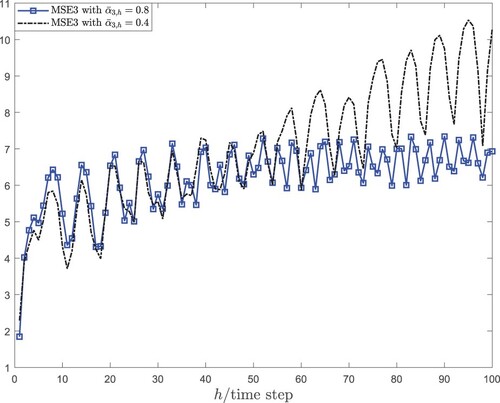MSE$j(j=1,2,3)$ are used to represent the mean square error for the jth node. The MSE and the corresponding upper bound are shown in Figure 5. To illustrate the effect of the time-delays on the estimation accuracy, the comparisons of the MSEj with ${\overline{\alpha }}_{i,h}=0.4$ and ${\overline{\alpha }}_{i,h}=0.8$ are presented in Figures 6–8.

Figure 1. The state and estimation trajectories of $x_{1,h}$.

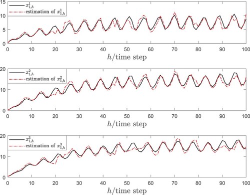
Figure 2. The state and estimation trajectories of $x_{2,h}$.

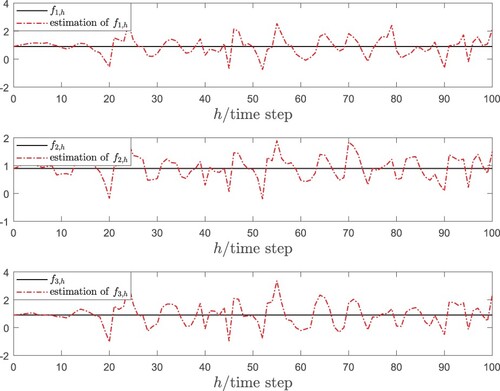
Figure 3. The state and estimation trajectories of $x_{3,h}$.

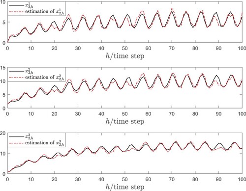
Figure 4. The real fault $f_{i,h}$ and its estimation.

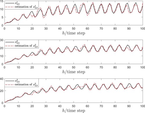
Figure 5. MSE and their upper bounds.

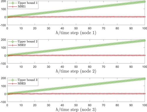
Figure 6. MSE1 with different ${\overline{\alpha }}_{1,h}$.

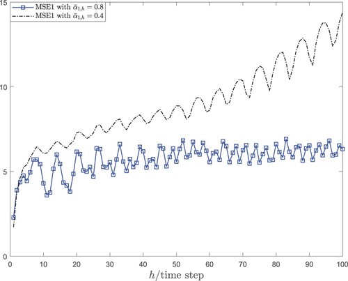
Figure 7. MSE2 with different ${\overline{\alpha }}_{2,h}$.

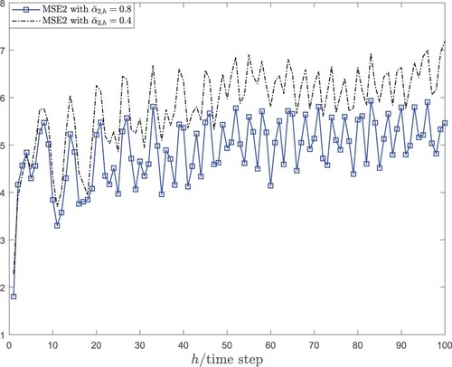
Figure 8. MSE3 with different ${\overline{\alpha }}_{3,h}$.

6. Conclusion

In this paper, the non-fragile joint state and fault estimation problem has been solved for NTVCNs with uncertain inner coupling and mixed time-delays. A novel joint estimation method has been designed, which can estimate the state and fault simultaneously. A set of zero-mean multiplicative noises has been used to characterize the variations of the estimator gain. The upper bound of the SEECM has been obtained, which can be minimized at each sampling instant via parameterizing the estimator gain properly. Moreover, a sufficient condition has been given to guarantee that the obtained upper bound is bounded. Finally, a numerical simulation has been given to illustrate the validity and effectiveness of the developed VCRSE algorithms. Based on the obtained results, the potential research directions include the design of the protocol-based VCRSE algorithm, such as the FlexRay protocol in Liu, Wang, Wang, et al. (2021) and adaptive event-triggered communication protocol in Wang et al. (2022).

Disclosure statement

No potential conflict of interest was reported by the author(s).

Additional information

Funding

This work was supported in part by the National Natural Science Foundation of China under Grant 72001059 and 12071102, the Key Foundation of Educational Science Planning in Heilongjiang Province of China under Grant GJB1422069, the Outstanding Youth Science Foundation of Heilongjiang Province of China under Grant YQ2020A004, and the University Nursing Program for Young Scholars with Creative Talents in Heilongjiang Province of China under Grant UNPYSCT-2020186.

References

- Chen, Y., Meng, X., Wang, Z., & Dong, H. (2021). Event-triggered recursive state estimation for stochastic complex dynamical networks under hybrid attacks. IEEE Transactions on Neural Networks and Learning Systems. https://doi.org/10.1109/TNNLS.2021.3105409.
- Dong, H., Hou, N., & Wang, Z. (2020). Fault estimation for complex networks with randomly varying topologies and stochastic inner couplings. Automatica, 112(11), 108734. https://doi.org/10.1016/j.automatica.2019.108734.
- Duan, P., Lv, G., Duan, Z., & Lv, Y. (2020). Resilient state estimation for complex dynamic networks with system model perturbation. IEEE Transactions on Control of Network Systems, 8(1), 135–146. https://doi.org/10.1109/TCNS.6509490
- Gao, H., Dong, H., Wang, Z., & Han, F. (2021). Recursive minimum-variance filter design for state-saturated complex networks with uncertain coupling strengths subject to deception attacks. IEEE Transactions on Cybernetics. https://doi.org/10.1109/TCYB.2021.3067822.
- Gao, M., Zhang, W., Sheng, L., & Zhou, D. (2020). Distributed fault estimation for delayed complex networks with round-robin protocol based on unknown input observer. Journal of the Franklin Institute, 357(13), 8678–8702. https://doi.org/10.1016/j.jfranklin.2020.04.012
- Geng, H., Liu, H., Ma, L., & Yi, X. (2021). Multi-sensor filtering fusion meets censored measurements under a constrained network environment: Advances, challenges and prospects. International Journal of Systems Science, 52(16), 3410–3436. https://doi.org/10.1080/00207721.2021.2005178
- Hou, N., Li, J., Liu, H., Ge, Y., & Dong, H. (2022). Finite-horizon resilient state estimation for complex networks with integral measurements from partial nodes. Science China Information Sciences, 65(3), 1–15. https://doi.org/10.1007/s11432-020-3243-7
- Hu, J., Jia, C., Liu, H., Yi, X., & Liu, Y. (2021). A survey on state estimation of complex dynamical networks. International Journal of Systems Science, 52(16), 3351–3367. https://doi.org/10.1080/00207721.2021.1995528
- Hu, J., Wang, Z., Liu, G.-P., & Zhang, H. (2020). Variance-constrained recursive state estimation for time-varying complex networks with quantized measurements and uncertain inner coupling. IEEE Transactions on Neural Networks and Learning Systems, 31(6), 1955–1967. https://doi.org/10.1109/TNNLS.5962385
- Huang, C., Xiong, Y., & Wang, W. (2021). Partial-information-based synchronization of complex networks with multiple and event-triggered couplings. Complexity, 2021(3), 1–14. Article No. 6613435.https://doi.org/10.1155/2021/6613435.
- Jia, C., Hu, J., Lv, C., & Shi, Y. (2020). Optimized state estimation for nonlinear dynamical networks subject to fading measurements and stochastic coupling strength: An event-triggered communication mechanism. Kybernetika, 56(1), 35–56. https://doi.org/10.14736/kyb-2020-1-0035
- Ju, Y., Tian, X., Liu, H., & Ma, L. (2021). Fault detection of networked dynamical systems: A survey of trends and techniques. International Journal of Systems Science, 52(16), 3390–3409. https://doi.org/10.1080/00207721.2021.1998722
- Li, J., Wang, Z., Hu, J., Liu, H., & Yi, X. (2022). Communication-protocol-based distributed filtering for general systems over sensor networks: Developments and challenges. International Journal of General Systems. https://doi.org/10.1080/03081079.2022.2052063.
- Li, J.-Y., Wang, Z., Lu, R., & Xu, Y. (2021). Partial-nodes-based state estimation for complex networks with constrained bit rate. IEEE Transactions on Network Science and Engineering, 8(2), 1887–1899. https://doi.org/10.1109/TNSE.2021.3076113
- Li, Q., Shen, B., Wang, Z., Huang, T., & Luo, J. (2019). Synchronization control for a class of discrete time-delay complex dynamical networks: A dynamic event-triggered approach. IEEE Transactions on Cybernetics, 49(5), 1979–1986. https://doi.org/10.1109/TCYB.6221036
- Li, X., & Xu, S. (2021). Multi-sensor complex network data fusion under the condition of uncertainty of coupling occurrence probability. IEEE Sensors Journal, 21(22), 24933–24940. https://doi.org/10.1109/JSEN.2021.3061437
- Liu, D., Wang, Z., Liu, Y., Alsaadi, F. E., & Alsaadi, F. E. (2021). Recursive state estimation for stochastic complex networks under round-robin communication protocol: Handling packet disorders. IEEE Transactions on Network Science and Engineering, 8(3), 2455–2468. https://doi.org/10.1109/TNSE.2021.3095217
- Liu, L., Zhang, Y., Zhou, W., Ren, Y., & Li, X. (2020). Event-triggered approach for finite-time state estimation of delayed complex dynamical networks with random parameters. International Journal of Robust and Nonlinear Control, 30(14), 5693–5711. https://doi.org/10.1002/rnc.v30.14
- Liu, S., Wang, Z., Wang, L., & Wei, G. (2021). Recursive set-membership tate estimation over a FlexRay network. IEEE Transactions on Systems, Man, and Cybernetics: Systems. https://doi.org/10.1109/TSMC.2021.3071390.
- Liu, Y., Shen, B., & Sun, J. (2021). Stubborn state estimation for complex-valued neural networks with mixed time delays: The discrete time case. Neural Computing and Applications, 34(7), 5449–5464. https://doi.org/10.1007/s00521-021-06707-y
- Liu, Y., Wang, Z., Zou, L., Zhou, D., & Chen, W.-H. (2022). Joint state and fault estimation of complex networks under measurement saturations and stochastic nonlinearities. IEEE Transactions on Signal and Information Processing Over Networks, 8, 173–186. https://doi.org/10.1109/TSIPN.2022.3150183
- Luo, Y., Wang, Z., Chen, Y., & Yi, X. (2021). H∞ state estimation for coupled stochastic complex networks with periodical communication protocol and intermittent nonlinearity switching. IEEE Transactions on Network Science and Engineering, 8(2), 1414–1425. https://doi.org/10.1109/TNSE.2021.3058220
- Ma, L., Wang, Z., Liu, Y., & Alsaadi, F. E. (2019). Distributed filtering for nonlinear time-delay systems over sensor networks subject to multiplicative link noises and switching topology. International Journal of Robust and Nonlinear Control, 29(10), 2941–2959. https://doi.org/10.1002/rnc.v29.10
- Mao, J., Sun, Y., Yi, X., Liu, H., & Ding, D. (2021). Recursive filtering of networked nonlinear systems: A survey. International Journal of Systems Science, 52(6), 1110–1128. https://doi.org/10.1080/00207721.2020.1868615
- Peng, H., Lu, R., Xu, Y., & Yao, F. (2018). Dissipative non-fragile state estimation for Markovian complex networks with coupling transmission delays. Neurocomputing, 275(8), 1576–1584. https://doi.org/10.1016/j.neucom.2017.09.096
- Shen, B., Wang, Z., & Qiao, H. (2017). Event-triggered state estimation for discrete-time multidelayed neural networks with stochastic parameters and incomplete measurements. IEEE Transactions on Neural Networks and Learning Systems, 28(5), 1152–1163. https://doi.org/10.1109/TNNLS.2016.2516030
- Shen, B., Wang, Z., Wang, D., & Li, Q. (2020). State-saturated recursive filter design for stochastic time-varying nonlinear complex networks under deception attacks. IEEE Transactions on Neural Networks and Learning Systems, 31(10), 3788–3800. https://doi.org/10.1109/TNNLS.5962385
- Shen, H., Hu, X., Wu, X., He, S., & Wang, J. (2022). Generalized dissipative state estimation of singularly perturbed switched complex dynamic networks with persistent dwell-time mechanism. IEEE Transactions on Systems, Man, and Cybernetics: Systems, 52(3), 1795–1806. https://doi.org/10.1109/TSMC.2020.3034635
- Sheng, L., Niu, Y., Zou, L., Liu, Y., & Alsaadi, F. E. (2018). Finite-horizon state estimation for time-varying complex networks with random coupling strengths under Round-Robin protocol. Journal of the Franklin Institute, 355(15), 7417–7442. https://doi.org/10.1016/j.jfranklin.2018.07.026
- Tan, Y., Xiong, M., Zhang, B., & Fei, S. (2021). Adaptive event-triggered nonfragile state estimation for fractional-order complex networked systems with cyber attacks. IEEE Transactions on Systems, Man, and Cybernetics: Systems. 52(4), 2121–2133. https://doi.org/10.1109/TSMC.2021.3049231.
- Wang, J.-L., Zhang, X.-X., Wen, G., Chen, Y., & Wu, H.-N. (2021). Passivity and finite-time passivity for multi-weighted fractional-order complex networks with fixed and adaptive couplings. IEEE Transactions on Neural Networks and Learning Systems. https://doi.org/10.1109/TNNLS.2021.3103809.
- Wang, L., Liu, S., Zhang, Y., Ding, D., & Yi, X. (2022). Non-fragile l2- l∞ state estimation for time-delayed artificial neural networks: An adaptive event-triggered approach. International Journal of Systems Science. https://doi.org/10.1080/00207721.2022.2049919.
- Wang, L., Wang, Z., Huang, T., & Wei, G. (2016). An event-triggered approach to state estimation for a class of complex networks with mixed time delays and nonlinearities. IEEE Transactions on Cybernetics, 46(11), 2497–2508. https://doi.org/10.1109/TCYB.2015.2478860
- Wang, S. (2019). Adaptive synchronisation of complex networks with non-dissipatively coupled and uncertain inner coupling matrix. Pramana-Journal of Physics, 93(1), 1–10. https://doi.org/10.1007/s12043-019-1748-9
- Yu, L., Liu, Y., Cui, Y., Alotaibi, N. D., & Alsaadi, F. E. (2021). Intermittent dynamic event-triggered state estimation for delayed complex networks based on partial nodes. Neurocomputing, 459(11), 59–69. https://doi.org/10.1016/j.neucom.2021.06.017
- Zhang, X.-M., Han, Q.-L., Wang, Z., & Zhang, B.-L. (2017). Neuronal state estimation for neural networks with two additive time-varying delay components. IEEE Transactions on Cybernetics, 47(10), 3184–3194. https://doi.org/10.1109/TCYB.2017.2690676
- Zou, L., Wang, Z., Gao, H., & Liu, X. (2017). State estimation for discrete-time dynamical networks with time-varying delays and stochastic disturbances under the Round-Robin protocol. IEEE Transactions on Neural Networks and Learning Systems, 28(5), 1139–1151. https://doi.org/10.1109/TNNLS.5962385
- Zou, L., Wang, Z., Han, Q.-L., & Zhou, D. H. (2021). Moving horizon estimation of networked nonlinear systems with random access protocol. IEEE Transactions on Systems, Man, and Cybernetics: Systems, 51(5), 2937–2948. https://doi.org/10.1109/TSMC.2019.2918002
- Zou, L., Wang, Z., Hu, J., & Dong, H. (2022). Partial-node-based state estimation for delayed complex networks under intermittent measurement outliers: A multiple-order-holder approach. IEEE Transactions on Neural Networks and Learning Systems. https://doi.org/10.1109/TNNLS.2021.3138979.
- Zou, L., Wang, Z., Hu, J., Liu, Y., & Liu, X. (2021). Communication-protocol-based analysis and synthesis of networked systems: Progress, prospects and challenges. International Journal of Systems Science, 52(14), 3013–3034. https://doi.org/10.1080/00207721.2021.1917721