Stability analysis of low-voltage direct current system with time-varying delay

ABSTRACT

This paper investigates the stability analysis of LVDC systems with time-varying delay. A hierarchical control model is constructed for LVDC systems subjected to time-varying delay. Furthermore, a novel Lyapunov-Krasovskii functional is developed by introducing the augmented terms and the delay-dependent matrices. To reduce the conservativeness of stability criteria, the constructed functional is effectively estimated by using the quadratic function inequalities and composite relaxation integral inequalities. Finally, the simulation results are given to validate the proposed method with a higher time-delay stability margin of LVDC systems.

KEYWORDS:

• Low-voltage direct current (LVDC) systems
• time-varying delay
• hierarchical control
• Lyapunov-Krasovskii functional

1. Introduction

Low-voltage direct current (LVDC) systems offer some advantages, such as high efficiency, low losses, reliability and better integration of renewable energy (Hong et al., 2023; Zhao et al., 2022). So LVDC systems are widely utilized in urban grids, electric vehicle charging stations, and distributed energy systems (Castillo-Calzadilla et al., 2022; Miranda et al., 2022; Purgat et al., 2023). Compared with traditional alternating current distribution networks, LVDC systems can effectively reduce energy conversion losses during DC loads and renewable energy access while possessing structural diversity, high flexibility and controllability (Seo et al., 2023; Zhang et al., 2023). However, the uncertainty of renewable energy and the changes of DC loads lead to fluctuations in the DC voltage of LVDC systems (Hussain et al., 2018). Besides, the transmission of control signals depends on the communication network, and time-delay is generated in the process of data network transmission inevitably due to the transmission speed and network congestion (Luo & Hu, 2022; Vafamand et al., 2019). It is well known that the above problems have a non-negligible impact on the stability of LVDC systems.

The stability problem of LVDC systems has always been a research focus in the field of electrical engineering and control, which can be made mainly on two aspects, one is to address the voltage fluctuation within the LVDC systems. An improved additional control strategy was proposed by controlling the operating region based on a minor damping power to stabilize the DC voltage of the LVDC systems (Deng et al., 2023). Deng et al. (2018) and Magne et al. (2012) designed the stabilizing feedback laws to apply additional current control at the converter station for LVDC systems, which can effectively mitigate the DC voltage fluctuation and enhance the system stability. In Liu et al. (2023), a converter control strategy, based on the droop control, was proposed by altering the droop coefficient to suppress the DC voltage fluctuations which is caused by power disturbances. Considering the influence of load mutation on the stability of LVDC systems, Zhang et al. (2019) proposed an improved droop control strategy, which ensured the control accuracy and enhanced the stability of the system. The other aspect is to address the influence of communication delays within the LVDC systems. Coelho et al. (2016) introduced a control strategy incorporating load frequency control and a single-time-delay communication network, involving external power controllers, internal voltage and current controllers to multiple parallel inverters. In addition, Heydari et al. (2019) combined time-delay model predictions with supplementary control to analyse the time-delay stability of multi-terminal LVDC systems. Lv et al. (2021) provided a distributed secondary control approach for LVDC systems, constructed a small-signal analysis model with communication delays and analysed the impact of time-delay on system stability in the time domain. It is worth noting that most of literatures primarily focused on stability analysis under the constant time-delay and time-delay-free conditions. The time-varying delay considered in this paper can better reflect characteristic of the actual operating scenarios.

LVDC systems using open communication channels belong to typical time-delay systems, and the stability is typically analysed by using Lyapunov functional methods combined with linear matrix inequalities (Xiong et al., 2018). However, the stability criteria obtained by using Lyapunov-Krasovskii Functional (LKF) are sufficient conditions and tend to be somewhat conservative (Qian et al., 2021). To mitigate the conservativeness of the conclusions, it is crucial to construct an appropriate LKF, and addressing the integral terms generated during the differentiation of the LKF is also of paramount importance (Qian et al., 2020, 2022). Existing research builds upon Lyapunov stability theory and introduces several newer functional forms and integral inequalities (Lin et al., 2019; Peyghami et al., 2019). However, it's worth noting that the communication delays considered in the referenced studies fall within the category of constant delays.

Inspired by the above discussion, the stability issue of LVDC systems with time-varying delay is studied in this paper. Based on the small-signal analysis, an LVDC system model with time-varying delay is constructed. Subsequently, a novel Lyapunov-Krasovskii functional is designed, which incorporates augmented terms and time-delay-dependent matrices. The quadratic inequalities and the composite relaxation integral inequalities are utilized to enhance the accuracy of functional derivative estimation and improve the precision. Then, a stability criterion with lower conservatism is obtained. Finally, the effectiveness and superiority of the proposed methods is validated by a practical example.

The main technical contributions of this work are the following: (1) A hierarchical control-based LVDC system is proposed, and its small-signal and time-delayed system models are constructed. The balance of power and voltage are maintained through a local control layer. Meanwhile, the system’s rapid response capability to disturbances is enhanced through a central controller in the secondary optimization layer. (2) New augmented vectors are introduced into the constructed Lyapunov-Krasovskii functional, and more connections are established between different cross-vectors. It is crucial in achieving more significant time-delay stability margins for LVDC systems which are affected by time-varying delays. (3) The time-delay-dependent matrices are incorporated in scaling the Lyapunov-Krasovskii functional, and more extensive use of time-delay boundary information is made. It allows for generating additional cross-term combinations related to time delays after differentiation, further contributing to achieving larger time-delay stability margins for LVDC systems.

2. Problem formulation and preliminaries

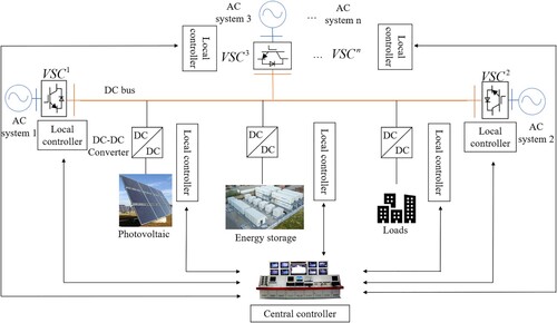
A typical LVDC system structure is shown in Figure 1, which generally consists of multiple converter stations, renewable energy generation units, and energy storage units. At the top level of the system, the control strategy layer is used in the central controller, to collect state variable information from local controllers of each device, and send control commands to the local devices while issuing control commands to the local controllers of each device simultaneously. This processing facilitates real-time monitoring of the DC bus voltage and the maintenance of the system power balance. In actual scenarios, due to a particular physical distance between local controllers and the central controller, a communication delay occurs during the transmission of control commands from the central controller to the local controllers. In LVDC system, considering different operating conditions and physical distances, communication delays typically range from a few milliseconds to several hundred milliseconds (Chen & Zhao, 2018).

Figure 1. Structure of the LVDC system.

In this section, two reasonable assumptions are made when constructing the LVDC system:

1. The VSCs in the LVDC system are connected to a strong AC grid on the AC side, and the impact of phase-locked loops is neglected in the modelling and analysis processes (Deng et al., 2022; Du et al., 2013).

2. The DC-DC converters in the LVDC system exhibit constant power load characteristics when operating in closed-loop control (Chia et al., 2015), so that the energy storage, photovoltaic (PV) generation units, and DC loads can be equivalently modelled as constant power loads $P_{eq}$.

For assumption 1, LVDC system typically operates at lower voltage levels. Unlike high-voltage direct current (HVDC) system, it does not necessitate a strong emphasis on the synchronicity of frequency and phase in grid connections. Additionally, LVDC system exhibits a certain tolerance for deviations. Therefore, the influence of phase-locked loops can be disregarded in the general modelling and analysis of LVDC system. Regarding assumption 2, the DC-DC converters employed in LVDC system operate in a closed-loop control manner, which implies that the system adjusts and maintains specific parameters through feedback mechanisms to achieve desired performance. In such a scenario, due to the flexible regulation of DC-DC converters, photovoltaic generation units, energy storage, and DC loads can be effectively aggregated and equivalently represented as a power load, exhibiting characteristics of constant power load within a specific range.

In this study, the variability and intermittency of PV generation units are considered as disturbance variables in the LVDC system, along with the power fluctuations of DC loads. These fluctuations in active power can impact the voltage stability and power balance of the LVDC system.

The LVDC system with hierarchical control is studied in this paper. The local control layer consists of $VSC$, PV generation units, energy storage, and DC loads, these equipped with local controllers. The master-slave control is used in the $VSC$ suggested in Chia et al. (2015). Within the LVDC system, the unique master station $VS{C}^1$ is implemented with a dual closed-loop control strategy based on outer voltage control and inner current control to maintain voltage stability. 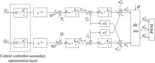The remaining $VSC$ are slave stations and a dual closed-loop control strategy with a power outer loop and a current inner loop is implemented to maintain constant power. Power disturbance signals are transmitted to the secondary optimization layer when fluctuations occur in the PV generation units or DC loads. The secondary optimization layer utilizes the central controller further to optimize system power and voltage via the communication network. Control block diagrams of the master station $VS{C}^1$ and the slave station $VSC$ are shown in Figures 2 and 3, respectively.

Figure 2. Block diagram of master $VSC$ constant DC voltage control.

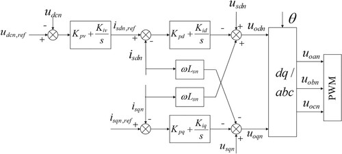
Figure 3. Block diagram of slave $VSC$ constant power control.

where $K_{pu}$, $K_{iu}$ are the proportional and integral control parameters of the voltage outer loop in the constant voltage control; $K_{pP}$, $K_{pQ}$, $K_{iP}$ and $K_{iQ}$ are the proportional and integral control parameters of the power outer loop in constant power control; $K_{pd}$, $K_{pq}$, $K_{id}$ and $K_{iq}$ are the proportional and integral control parameters of the current inner loop in the dq-axis; $K_p^P$, $K_i^P$, $K_p^Q$ and $K_i^Q$ are the embedded proportional and integral control parameters in the central controller; $u_{sd}^n$, $u_{sq}^n$ are the dq-axis components of the three-phase voltage on the AC side of $VS{C}^n$; $i_{sd}^n$, $i_{sq}^n$ are the dq-axis components of the three-phase current on the AC side of $VS{C}^n$; $u_{od}^n$, $u_{oq}^n$ are the dq-axis reference values of the three-phase voltage on the bridge arm side of $VS{C}^n$; $P_{CE}$, $Q_{CE}$ are the active and reactive power deviations input to the central controller from the LVDC system; $\mathrm{\Delta }{P}^{n\ast }$, $\mathrm{\Delta }{Q}^{n\ast }$ are the secondary optimization control commands for active and reactive power obtained through embedded central controller computation; $P^n$, $Q^n$ are the actual values of active and reactive power.

To simplify the modelling process, this paper takes a two-terminal LVDC system, and a hierarchical control model of the LVDC system considering communication delays is constructed by small-signal analysis. The simplified LVDC system model constructed in this paper comprises the main VSC model, the slave VSC model, and the direct current network model (Castro, 2022; Gerber et al., 2022; Hallemans et al., 2022). The detailed derivation process and complete expressions are provided in the Appendix.

When communication delays are not considered, the model of the two-terminal LVDC system is indicated as: (1) $\frac{dx\left(t\right)}{dt}=A_{s}x\left(t\right)+A_{ds}x\left(t\right)+B_s\mathrm{\Delta }{u}_{ds}\left(t\right)$(1) where $x$ is the state variables of the LVDC system, $x=[x_m^1{x}_n^2{x}_g{]}^T$; $x_n^2$ is the state variables of the slave station, $x_n^2=[\mathrm{\Delta }{u}_{dc}^2\mathrm{\Delta }{i}_{sd}^2\mathrm{\Delta }{i}_{sq}^2\mathrm{\Delta }{W}_P^2\mathrm{\Delta }{W}_Q^2\mathrm{\Delta }{W}_d^2\mathrm{\Delta }{W}_q^2\mathrm{\Delta }{W}_P^{\ast }\mathrm{\Delta }{W}_Q^{\ast }{]}^T$; $x_m^1$ is the state variables of the master station, $x_m^1=[\mathrm{\Delta }{u}_{dc}^1\mathrm{\Delta }{i}_{sd}^1\mathrm{\Delta }{i}_{sq}^1\mathrm{\Delta }{W}_{ud}^1\mathrm{\Delta }{W}_{uq}^1\mathrm{\Delta }{W}_d^1\mathrm{\Delta }{W}_q^1{]}^T$; $x_g$ is the state variables of the network, $x_g=[\mathrm{\Delta }{u}_{dc}\mathrm{\Delta }{i}_1\mathrm{\Delta }{i}_2{]}^T$; $\mathrm{\Delta }{W}_P^2,\mathrm{\Delta }{W}_Q^2,\mathrm{\Delta }{W}_d^2,\mathrm{\Delta }{W}_q^2$ are the integral elements of outer voltage loop and inner current loop in the slave station respectively; $\mathrm{\Delta }{W}_P^{\ast },\mathrm{\Delta }{W}_Q^{\ast }$ are the integral elements in central controller respectively; $\mathrm{\Delta }{W}_{ud}^1,\mathrm{\Delta }{W}_{uq}^1,\mathrm{\Delta }{W}_d^1,\mathrm{\Delta }{W}_q^1$ are the integral elements of outer power loop and inner current loop in the master station respectively; $\mathrm{\Delta }{u}_{ds}$ is the disturbance variables, $\mathrm{\Delta }{u}_{ds}=\left[\mathrm{\Delta }{P}_{eq}\right]$; $A_s,A_{ds},B_s$ are the state matrix, the input matrix and the disturbance matrix of the two-terminal LVDC system; $A_n^2,A_{dn}^2$ are the state matrix and the input matrix of the slave station; $A_m^1$ is the state matrix of the master station; $A_g,B_{ds}$ are the state matrix, the input matrix and the disturbance matrix of the LVDC system network.

where $\begin{array}{rl}{A}_L& =\left[\begin{array}{cc}{0}_{(1\times 9)}& 0_{(1\times 7)}\\ \left[\begin{array}{cc}{\displaystyle \frac{1}{L_1}}& 0_{(1\times 8)}\end{array}\right]& 0_{(1\times 7)}\\ 0_{(1\times 9)}& \left[\begin{array}{cc}{\displaystyle \frac{1}{L_2}}& 0_{(1\times 6)}\end{array}\right]\end{array}\right],\\ A_C& =\left[\begin{array}{ccc}{0}_{(9\times 1)}& \left[\begin{array}{c}-{\displaystyle \frac{1}{C_1}}\\ 0_{(8\times 1)}\end{array}\right]& 0_{(9\times 1)}\\ 0_{(7\times 1)}& 0_{(7\times 1)}& \left[\begin{array}{c}-{\displaystyle \frac{1}{C_2}}\\ 0_{(6\times 1)}\end{array}\right]\end{array}\right]\end{array}$A specific physical distance exists between the central and local controllers in the actual scenario. The power outer-loop PI controller of the slave station $VS{C}^2$ experiences communication delays when receiving power secondary optimization control commands from the central controller, which affects the control effect of the secondary optimization layer.

Therefore, the communication delays generated from the central controller output $\mathrm{\Delta }{u}_n^2={\left[\begin{array}{cc}\mathrm{\Delta }{P}^{2\ast }& \mathrm{\Delta }{Q}^{2\ast }\end{array}\right]}^T$ to the input of the slave station $VS{C}^2$ is denoted as $e^{-sh}$, $h$ is the upper bound of the time-delay, and $s$ is the Laplace operator. Simultaneously, as observed from Figure 3, the slave station $VS{C}^2$ is influenced by communication delays, whereas the main station $VS{C}^1$ and relevant state variables of the system's DC network are unaffected by communication delays. Thus, to facilitate analysis, the mathematical model can be expressed as: (2) $\dot{x}\left(t\right)=Ax\left(t\right)+A_{d}x(t-h(t\left)\right)+K\mathrm{\Delta }{u}_{ds}\left(t\right)$(2) where $A=A_s$, $A_d=A_{ds}$, $K=B_s$.

Also, time-varying delays satisfy: $0\le h\left(t\right)\le h$, $\dot{h}\left(t\right)\le \mu$.

The nonlinear disturbance $\mathrm{\Delta }{u}_{ds}$ of the LVDC system is shown as the following format: (3) $K\mathrm{\Delta }{u}_{ds}\left(t\right)=f(t,x(t),x(t-h\left(t\right)\left)\right)$(3) And it satisfies the following bounded-norm conditions: (4) $\Vert f(\cdot )\Vert \le \overline{\alpha }\Vert x\left(t\right)\Vert +\overline{\text{β}}\Vert x(t-h(t\left)\right)\Vert$(4) where $\overline{\alpha }\ge 0$ and $\overline{\text{β}}\ge 0$ are known scalars in the following expansion formats: (5) $\begin{array}{rl}f(\cdot {)}^{T}f(\cdot )& \le {\overline{\alpha }}^2{x}^T\left(t\right){\overline{Z}}^T\overline{Z}x\left(t\right)\\ & +{\overline{\text{β}}}^2{x}^T(t-h(t\left)\right){\overline{X}}^T\overline{X}x(t-h(t\left)\right)\end{array}$(5) where $\overline{Z}$ and $\overline{X}$ are constant matrices of appropriate dimensions.

The main objective of this paper is to derive the less conservatism criteria, and guarantee system (2) asymptotically stable. In order to obtain main results, the following lemmas are required.

Lemma 2.1

Zeng et al., 2019

Assume $N\in \mathbb{N}$, $\xi \in {\mathbb{R}}^m$, moreover, for a continuous differentiable function $x$: $\left[\alpha ,\text{β}\right]\to R^n$, the following inequality holds for any matrix $Z\left(\in {\mathbb{R}}^{n\times n}\right)>0$, $M\in {\mathbb{R}}^{\left(N+1\right)n\times m}$: $-{\int }_{\alpha }^{\text{β}}{\dot{x}}^{\text{T}}\left(u\right)Z\dot{x}\left(u\right)\text{d}u\le 2{\zeta }_N^T{\mathrm{\Gamma }}_N^{T}M\xi +(\text{β}-\alpha ){\xi }^T{M}^T\tilde{Z}M\xi$where the detailed definition of variables is shown in Zeng et al. (2019).

Lemma 2.2

Zeng et al., 2020

Given a quadratic function $\vartheta \left(x\right)=a_2{x}^2+a_{1}x+a_0$, where $a_i\in \mathbb{R}\left(i=0,1,2\right)$, if the following inequality holds: $\begin{array}{r}\begin{array}{cc}\left(\mathrm{i}\right)& \vartheta \left(0\right)<0,\\ \left(\mathrm{i}\mathrm{i}\right)& \vartheta \left(h\right)<0,\\ (\mathrm{i}\mathrm{i}\mathrm{i})& \frac{h}{4}{a}_1+a_0<0,\\ \left(\mathrm{i}\mathrm{v}\right)& \frac{h^2}{2}{a}_2+\frac{3h}{4}{a}_1+a_0<0\end{array}\end{array}$Then for $\mathrm{\forall }x\in \left[0,h\right]$, there exists $\vartheta \left(x\right)<0$.

3. Main results

In this section, a novel Lyapunov-Krasovskii functional is constructed with more time-delay information. A more innovative analytical approach is used to derive stability criteria for time-varying delayed LVDC system. Some notations for matrices and vectors are shown as follows: ${ϵ}_1\left(t\right)={\int }_{t-h\left(t\right)}^t{x}^T\left(s\right)ds,{ϵ}_2\left(t\right)={\int }_{t-h}^{t-h\left(t\right)}{x}^T\left(s\right)ds$ $\begin{array}{rl}{ϵ}_3\left(t\right)& =\frac{1}{h\left(t\right)}{\int }_{t-h\left(t\right)}^t{\int }_{\theta }^t{x}^T\left(s\right)dsd\theta ,\\ {ϵ}_4\left(t\right)& =\frac{1}{\left(h-h\left(t\right)\right)}{\int }_{t-h}^{t-h\left(t\right)}{\int }_{\theta }^{t-h\left(t\right)}{x}^T\left(s\right)dsd\theta ,\end{array}$ ${\eta }_0\left(t\right)={\left[\begin{array}{ccc}{x}^T\left(t\right)& x^T\left(t-h\left(t\right)\right)& x^T\left(t-h\right)\end{array}\right]}^T,$ ${\eta }_1\left(t\right)={\left[\begin{array}{cc}\begin{array}{cccc}{\eta }_0^T\left(t\right)& {ϵ}_1^T\left(t\right)& {ϵ}_2^T\left(t\right)& {ϵ}_3^T\end{array}\left(t\right)& {ϵ}_4^T\left(t\right)\end{array}\right]}^T,$ ${\eta }_2\left(t\right)={\left[\begin{array}{ccc}{\eta }_0^T\left(t\right)& \frac{1}{h\left(t\right)}{ϵ}_1^T\left(t\right)& \frac{1}{h\left(t\right)}{ϵ}_3^T\left(t\right)\end{array}\right]}^T,$ ${\eta }_3\left(t\right)={\left[\begin{array}{ccc}{\eta }_0^T\left(t\right)& \frac{1}{h-h\left(t\right)}{ϵ}_2^T\left(t\right)& \frac{1}{h-h\left(t\right)}{ϵ}_4^T\left(t\right)\end{array}\right]}^T,$ ${\eta }_4\left(t,s\right)={\left[\begin{array}{cccc}{\dot{x}}^T\left(s\right)& x^T\left(s\right)& {\int }_s^t{x}^T\left(\theta \right)d\theta & {\int }_{t-h\left(t\right)}^s{x}^T\left(\theta \right)d\theta \end{array}\right]}^T,$ $\begin{array}{rl}{\eta }_5\left(t,s\right)& =[{\dot{x}}^T\left(s\right)x^T\left(s\right){\int }_s^{t-h\left(t\right)}{x}^T\left(\theta \right)d\theta \\ & {{\int }_{t-h}^s{x}^T\left(\theta \right)d\theta ]}^T,\end{array}$ $\begin{array}{rl}\xi \left(t\right)& ={\left[\begin{array}{ccc}{\eta }_0^T\left(t\right)& {\xi }_1^T\left(t\right)& {\xi }_2^T\left(t\right)\end{array}\right]}^T,\\ {\xi }_1\left(t\right)& ={\left[\begin{array}{ccc}{\dot{x}}^T\left(t-h\left(t\right)\right)& {\dot{x}}^T\left(t-h\right)& \frac{1}{h\left(t\right)}{ϵ}_1^T\left(t\right)\end{array}\right]}^T,\end{array}$ ${\xi }_2\left(t\right)={\left[\begin{array}{ccc}\frac{1}{h-h\left(t\right)}{ϵ}_2^T\left(t\right)& \frac{1}{h\left(t\right)}{ϵ}_3^T\left(t\right)& \frac{1}{h-h\left(t\right)}{ϵ}_4^T\left(t\right)\end{array}\right]}^T,$ $\begin{array}{rl}{e}_i& =\left[\begin{array}{ccc}{0}_{n\times \left(i-1\right)n}& I_n& 0_{n\times \left(9-i\right)n}\end{array}\right],\\ & i=1,2,\dots ,9,e_0=A{e}_1+A_d{e}_2\end{array}$

Theorem 3.1:

For given positive scalars $h>0$ and $\mu <1$, if there exist positive definite symmetric matrices $U\in {\mathbb{R}}^{9n\times 9n}$, $Q_1\in {\mathbb{R}}^{4n\times 4n}$, $Q_2\in {\mathbb{R}}^{4n\times 4n}$, $R_1\in {\mathbb{R}}^{n\times n}$, $R_2\in {\mathbb{R}}^{n\times n}$, symmetric matrices $P_{11}\in {\mathbb{R}}^{5n\times 5n}$, $P_{12}\in {\mathbb{R}}^{5n\times 5n}$, $P_{21}\in {\mathbb{R}}^{5n\times 5n}$, $P_{22}\in {\mathbb{R}}^{5n\times 5n}$, and matrices $N_1$, $N_2$ of appropriate dimensions, such that for $\mathrm{\forall }h\left(t\right)\in \left[0,h\right]$ and $\dot{h}\left(t\right)\le \mu$, the following LMIs hold, then system (2) is asymptotically stable: (6) $\begin{array}{rl}\left[\begin{array}{cc}\mathrm{\Xi }\left(h\left(t\right),\dot{h}\left(t\right)\right)& h^{\frac{1}{2}}{N}_2\\ \ast & -{\hat{R}}_1\end{array}\right]& <0\end{array}$(6) (7) $\begin{array}{rl}\left[\begin{array}{cc}\mathrm{\Xi }\left(h\left(t\right),\dot{h}\left(t\right)\right)& h^{\frac{1}{2}}{N}_1\\ \ast & -{\hat{R}}_2\end{array}\right]& <0\end{array}$(7) (8) $\begin{array}{rl}{P}_{11}+h\left(t\right)P_{12}& >0\end{array}$(8) (9) $\begin{array}{rl}{P}_{21}+(h-h(t\left)\right)P_{22}& >0\end{array}$(9) where $\begin{array}{rl}\mathrm{\Xi }\left(h\left(t\right),\dot{h}\left(t\right)\right)& ={\gamma }_0\left(\dot{h}\left(t\right)\right)+h\left(t\right){\gamma }_1\left(\dot{h}\left(t\right)\right)+h^2\left(t\right){\gamma }_2\left(\dot{h}\left(t\right)\right),\end{array}$ $\begin{array}{rl}{\gamma }_0\left(\dot{h}\left(t\right)\right)& ={\delta }_0\left(\dot{h}\left(t\right)\right)+{\rho }_0\left(\dot{h}\left(t\right)\right),{\gamma }_1\left(\dot{h}\left(t\right)\right)\\ & ={\delta }_1\left(\dot{h}\left(t\right)\right)+{\rho }_1\left(\dot{h}\left(t\right)\right),\end{array}$ ${\rho }_0\left(\dot{h}\left(t\right)\right)=h{N}_2{\hat{R}}_1^{-1}{N}_2^{\text{T}},{\rho }_1\left(\dot{h}\left(t\right)\right)=N_1{\hat{R}}_2^{-1}{N}_1^{\text{T}}-N_2{\hat{R}}_1^{-1}{N}_2^{\text{T}},$ $\begin{array}{rl}{\gamma }_2\left(h\right(t\left)\right)& =\text{Sym}\{{\mathrm{\Pi }}_{11}^{\text{T}}{P}_{12}{\lambda }_1+{\mathrm{\Pi }}_{21}^{\text{T}}{P}_{22}{\lambda }_1\\ & +{\mathrm{\Pi }}_{53}^{\text{T}}{Q}_1{\lambda }_4+{\mathrm{\Pi }}_{83}^{\text{T}}{Q}_2{\lambda }_5\}\\ & -\left(1-\dot{h}\left(t\right)\right){\mathrm{\Pi }}_{42}^{\text{T}}{Q}_1{\mathrm{\Pi }}_{42}+{\mathrm{\Pi }}_{32}^{\text{T}}{Q}_1{\mathrm{\Pi }}_{32}\\ & -{\mathrm{\Pi }}_{72}^{\text{T}}{Q}_2{\mathrm{\Pi }}_{72}+\left(1-\dot{h}\left(t\right)\right){\mathrm{\Pi }}_{62}^{\text{T}}{Q}_2{\mathrm{\Pi }}_{62},\end{array}$ $\begin{array}{rl}{\delta }_0\left(h\right(t\left)\right)& =\dot{h}\left(t\right){\mathrm{\Pi }}_{11}^{\text{T}}{P}_{11}{\mathrm{\Pi }}_{11}-\dot{h}\left(t\right){\mathrm{\Pi }}_{21}^{\text{T}}\left(P_{21}+2h{P}_{22}\right){\mathrm{\Pi }}_{21}\\ & +{\mathrm{\Pi }}_{31}^{\text{T}}{Q}_1{\mathrm{\Pi }}_{31}-\left(1-\dot{h}\left(t\right)\right){\mathrm{\Pi }}_{41}^{\text{T}}{Q}_1{\mathrm{\Pi }}_{41}\\ & +\left(1-\dot{h}\left(t\right)\right){\mathrm{\Pi }}_{61}^{\text{T}}{Q}_2{\mathrm{\Pi }}_{61}\\ & -{\mathrm{\Pi }}_{71}^{\text{T}}{Q}_2{\mathrm{\Pi }}_{71}+h\left(1-\dot{h}\left(t\right)\right)e_4^{\text{T}}(R_1-R_2)e_4\\ & +h{e}_0^{\text{T}}{R}_2{e}_0+\text{Sym}\{{\mathrm{{\rm Y}}}_{12}^{T}U{o}_1+{\mathrm{\Pi }}_{11}^{\text{T}}{P}_{11}{\lambda }_2\\ & +{\mathrm{\Pi }}_{21}^{\text{T}}\left(h{P}_{21}+h^2{P}_{22}\right){\lambda }_1+{\mathrm{\Pi }}_{51}^{\text{T}}{Q}_1{\lambda }_4\\ & +{\mathrm{\Pi }}_{21}^{\text{T}}\left(P_{21}+h{P}_{22}\right){\lambda }_3\\ & +{\mathrm{\Pi }}_{81}^{\text{T}}{Q}_2{\lambda }_5+N_1{M}_1+N_2{M}_2\},\end{array}$ $\begin{array}{rl}{\delta }_1\left(h\left(t\right)\right)& =\text{Sym}\{{\mathrm{{\rm Y}}}_{11}^{T}U{o}_1+{\mathrm{\Pi }}_{11}^{\text{T}}{P}_{11}{\lambda }_1+{\mathrm{\Pi }}_{11}^{\text{T}}{P}_{12}{\lambda }_2\\ & -{\mathrm{\Pi }}_{21}^{\text{T}}\left(P_{21}+2h{P}_{22}\right){\lambda }_1-{\mathrm{\Pi }}_{21}^{\text{T}}{P}_{22}{\lambda }_3\\ & +{\mathrm{\Pi }}_{31}^{\text{T}}{Q}_1{\mathrm{\Pi }}_{32}-\left(1-\dot{h}\left(t\right)\right){\mathrm{\Pi }}_{41}^{\text{T}}{Q}_1{\mathrm{\Pi }}_{42}\\ & +{\mathrm{\Pi }}_{52}^{\text{T}}{Q}_1{\lambda }_4-{\mathrm{\Pi }}_{82}^{\text{T}}{Q}_2{\lambda }_5\\ & +\left(1-\dot{h}\left(t\right)\right){\mathrm{\Pi }}_{61}^{\text{T}}{Q}_2{\mathrm{\Pi }}_{62}-{\mathrm{\Pi }}_{71}^{\text{T}}{Q}_2{\mathrm{\Pi }}_{72}\}\\ & +2\dot{h}\left(t\right){\mathrm{\Pi }}_{11}^{\text{T}}{P}_{12}{\mathrm{\Pi }}_{11}+2\dot{h}\left(t\right){\mathrm{\Pi }}_{21}^{\text{T}}{P}_{22}{\mathrm{\Pi }}_{21}\\ & -\left(1-\dot{h}\left(t\right)\right)e_4^{\text{T}}\left(R_1-R_2\right)e_4\end{array}$where ${\mathrm{{\rm Y}}}_{11}^T={\left[\begin{array}{ccccccc}0& 0& 0& e_6^T& -e_7^T& e_8^T& -e_9^T\end{array}\right]}^T,$ ${\mathrm{{\rm Y}}}_{12}^T={\left[\begin{array}{ccccccc}{e}_1^T& e_2^T& e_3^T& 0& h{e}_7^T& 0& h{e}_9^T\end{array}\right]}^T,$ $\begin{array}{rl}{o}_1& =[e_0^T\left(1-\dot{h}\left(t\right)\right)e_4^T{e}_5^T{e}_1^T-\left(1-\dot{h}\left(t\right)\right)e_2^T\\ & \left(1-\dot{h}\left(t\right)\right)e_2^T-e_3^T{\nu }_1^T{\nu }_2^T{]}^T,\end{array}$ $\begin{array}{rl}{\nu }_1^T& =e_1^T-\left(1-\dot{h}\left(t\right)\right)e_6^T-\dot{h}\left(t\right)e_8^T,\\ {\nu }_2^T& =\left(1-\dot{h}\left(t\right)\right)e_2^T-e_7^T+\dot{h}\left(t\right)e_9^T,\end{array}$ $\begin{array}{rl}{\mathrm{\Pi }}_{11}& ={\left[\begin{array}{ccccc}{e}_1^{\text{T}}& e_2^{\text{T}}& e_3^{\text{T}}& e_6^{\text{T}}& e_8^{\text{T}}\end{array}\right]}^{\text{T}},\\ {\mathrm{\Pi }}_{21}& ={\left[\begin{array}{ccccc}{e}_1^{\text{T}}& e_2^{\text{T}}& e_3^{\text{T}}& e_7^{\text{T}}& e_9^{\text{T}}\end{array}\right]}^{\text{T}},\end{array}$ $\begin{array}{rl}{\mathrm{\Pi }}_{31}& ={\left[\begin{array}{cccc}{e}_0^{\text{T}}& e_1^{\text{T}}& 0& 0\end{array}\right]}^{\text{T}},{\mathrm{\Pi }}_{32}={\left[\begin{array}{cccc}0& 0& 0& e_6^{\text{T}}\end{array}\right]}^{\text{T}},\\ {\mathrm{\Pi }}_{41}& ={\left[\begin{array}{cccc}{e}_4^{\text{T}}& e_2^{\text{T}}& 0& 0\end{array}\right]}^{\text{T}},\end{array}$ $\begin{array}{rl}{\mathrm{\Pi }}_{42}& ={\left[\begin{array}{cccc}0& 0& e_6^{\text{T}}& 0\end{array}\right]}^{\text{T}},{\mathrm{\Pi }}_{51}={\left[\begin{array}{cccc}{e}_1^{\text{T}}-e_2^{\text{T}}& 0& 0& 0\end{array}\right]}^{\text{T}},\\ {\mathrm{\Pi }}_{52}& ={\left[\begin{array}{cccc}0& e_6^{\text{T}}& 0& 0\end{array}\right]}^{\text{T}},\end{array}$ $\begin{array}{r}{\mathrm{\Pi }}_{53}={\left[\begin{array}{cccc}0& 0& e_8^{\text{T}}& e_6^{\text{T}}-e_8^{\text{T}}\end{array}\right]}^{\text{T}},{\mathrm{\Pi }}_{61}={\left[\begin{array}{cccc}{e}_4^{\text{T}}& e_2^{\text{T}}& 0& h{e}_7^{\text{T}}\end{array}\right]}^{\text{T}},\end{array}$ $\begin{array}{rl}{\mathrm{\Pi }}_{62}& ={\left[\begin{array}{cccc}0& 0& 0& -e_7^{\text{T}}\end{array}\right]}^{\text{T}},{\mathrm{\Pi }}_{71}={\left[\begin{array}{cccc}{e}_5^{\text{T}}& e_3^{\text{T}}& h{e}_7^{\text{T}}& 0\end{array}\right]}^{\text{T}},\\ {\mathrm{\Pi }}_{72}& ={\left[\begin{array}{cccc}0& 0& -e_7^{\text{T}}& 0\end{array}\right]}^{\text{T}},\end{array}$ $\begin{array}{r}{\mathrm{\Pi }}_{81}={\left[\begin{array}{cccc}{e}_2^{\text{T}}-e_3^{\text{T}}& h{e}_7^{\text{T}}& h^2{e}_9^{\text{T}}& h^2(e_7^{\text{T}}-e_9^{\text{T}})\end{array}\right]}^{\text{T}},\end{array}$ $\begin{array}{rl}{\mathrm{\Pi }}_{82}& ={\left[\begin{array}{cccc}0& e_7^{\text{T}}& 2h{e}_9^{\text{T}}& 2h(e_7^{\text{T}}-e_9^{\text{T}})\end{array}\right]}^{\text{T}},\\ {\mathrm{\Pi }}_{83}& ={\left[\begin{array}{cccc}0& 0& e_9^{\text{T}}& e_7^{\text{T}}-e_9^{\text{T}}\end{array}\right]}^{\text{T}},\end{array}$ $\begin{array}{rl}{\tau }_1& ={\left[\begin{array}{cccc}0& 0& 0& e_1^{\text{T}}-(1-\dot{h}(t\left)\right)e_2^{\text{T}}-\dot{h}\left(t\right)e_6^{\text{T}}\end{array}\right]}^{\text{T}},\\ {\tau }_2& =[e_1^{\text{T}}-(1-\dot{h}(t\left)\right)e_6^{\text{T}}-2\dot{h}\left(t\right)e_8^{\text{T}}{]}^{\text{T}},\end{array}$ $\begin{array}{rl}{\tau }_3& ={\left[\begin{array}{cccc}0& 0& 0& (1-\dot{h}(t\left)\right)e_2^{\text{T}}-e_3^{\text{T}}+\dot{h}\left(t\right)e_7^{\text{T}}\end{array}\right]}^{\text{T}},\\ {\tau }_4& =[(1-\dot{h}(t\left)\right)e_2^{\text{T}}-e_7^{\text{T}}+2\dot{h}\left(t\right)e_9^{\text{T}}{]}^{\text{T}},\end{array}$ $\begin{array}{rl}{\lambda }_1& ={\left[\begin{array}{ccccc}{e}_0^{\text{T}}& (1-\dot{h}(t\left)\right)e_4^{\text{T}}& e_5^{\text{T}}& 0& 0\end{array}\right]}^{\text{T}},\\ {\lambda }_2& ={\left[\begin{array}{cc}{\tau }_1^{\text{T}}& {\tau }_2^{\text{T}}\end{array}\right]}^{\text{T}},{\lambda }_3={\left[\begin{array}{cc}{\tau }_3^{\text{T}}& {\tau }_4^{\text{T}}\end{array}\right]}^{\text{T}},\end{array}$ $\begin{array}{rl}{\lambda }_4& ={\left[\begin{array}{cccc}0& 0& e_1^{\text{T}}& -(1-\dot{h}(t\left)\right)e_2^{\text{T}}\end{array}\right]}^{\text{T}},\\ {\lambda }_5& ={\left[\begin{array}{cccc}0& 0& (1-\dot{h}(t\left)\right)e_2^{\text{T}}& -e_3^{\text{T}}\end{array}\right]}^{\text{T}},\end{array}$ $\begin{array}{r}{M}_1={\left[\begin{array}{ccc}{e}_1^{\text{T}}-e_2^{\text{T}}& e_1^{\text{T}}+e_2^{\text{T}}-2e_6^{\text{T}}& e_1^{\text{T}}-e_2^{\text{T}}+6e_6^{\text{T}}-12e_8^{\text{T}}\end{array}\right]}^{\text{T}},\end{array}$ $\begin{array}{r}{M}_2={\left[\begin{array}{ccc}{e}_2^{\text{T}}-e_3^{\text{T}}& e_2^{\text{T}}+e_3^{\text{T}}-2e_7^{\text{T}}& e_2^{\text{T}}-e_3^{\text{T}}+6e_7^{\text{T}}-12e_9^{\text{T}}\end{array}\right]}^{\text{T}},\end{array}$ $\begin{array}{r}{\hat{R}}_i=\text{diag}\left(R_i,3R_i,5R_i\right),i=1,2\end{array}$

Proof:

firstly, the Lyapunov-Krasovskii functional is constructed as follows: (10) $\begin{array}{rl}V(x_t,t)& =\sum _{i=1}^4{V}_i\left(x_t,t\right)\end{array}$(10) (11) $\begin{array}{rl}{V}_1\left(x_t,t\right)& ={\eta }_1^T\left(t\right)U{\eta }_1\left(t\right)\end{array}$(11) (12) $\begin{array}{rl}{V}_2\left(x_t,t\right)& =h\left(t\right){\eta }_2^T\left(t\right)P_1\left(t\right){\eta }_2\left(t\right)+\left(h-h\left(t\right)\right){\eta }_3^T\left(t\right)P_2\left(t\right){\eta }_3\left(t\right)\end{array}$(12) (13) $\begin{array}{rl}{V}_3\left(x_t,t\right)& ={\int }_{t-h\left(t\right)}^t{\eta }_4^T\left(t,s\right)Q_1{\eta }_4\left(t,s\right)ds\\ & +{\int }_{t-h}^{t-h\left(t\right)}{\eta }_5^T\left(t,s\right)Q_2{\eta }_5\left(t,s\right)ds\end{array}$(13) (14) $\begin{array}{rl}{V}_4\left(x_t,t\right)& ={\int }_{t-h}^{t-h\left(t\right)}\left(h-t+s\right){\dot{x}}^T\left(s\right)R_1\dot{x}\left(s\right)ds\\ & +{\int }_{t-h\left(t\right)}^t\left(h-t+s\right){\dot{x}}^T\left(s\right)R_2\dot{x}\left(s\right)ds\end{array}$(14) where $P_1\left(t\right)=P_{11}+h\left(t\right)P_{12}$, $P_2\left(t\right)=P_{21}+\left(h-h\left(t\right)\right)P_{22}$.

Taking the derivative of $V\left(x_t,t\right)$ along the trajectory of system(2) yields: (15) $\begin{array}{rl}{\dot{V}}_1\left(x_t,t\right)& =2{\eta }_1^T\left(t\right)U{\dot{\eta }}_1\left(t\right)\end{array}$(15) (16) $\begin{array}{rl}{\dot{V}}_2\left(x_t,t\right)& =2h\left(t\right){\eta }_2^{\text{T}}\left(t\right)P_1\left(t\right){\dot{\eta }}_2\left(t\right)+h\left(t\right){\eta }_2^{\text{T}}\left(t\right){\dot{P}}_1\left(t\right){\eta }_2\left(t\right)\\ & +\dot{h}\left(t\right){\eta }_2^{\text{T}}\left(t\right)P_1\left(t\right){\eta }_2\left(t\right)\\ & +2(h-h(t\left)\right){\eta }_3^{\text{T}}\left(t\right)P_2\left(t\right){\dot{\eta }}_3\left(t\right)\\ & +(h-h(t\left)\right){\eta }_3^{\text{T}}\left(t\right){\dot{P}}_2\left(t\right){\eta }_3\left(t\right)\\ & -\dot{h}\left(t\right){\eta }_3^{\text{T}}\left(t\right)P_2\left(t\right){\eta }_3\left(t\right)\end{array}$(16) (17) $\begin{array}{rl}{\dot{V}}_3\left(x_t,t\right)& ={\eta }_4^{\text{T}}(t,t)Q_{\text{l}}{\eta }_4(t,t)-{\eta }_5^{\text{T}}(t,t-h)Q_2{\eta }_5(t,t-h)\\ & -(1-\dot{h}(t\left)\right){\eta }_4^{\text{T}}(t,t-h(t\left)\right)Q_1{\eta }_4(t,t-h(t\left)\right)\\ & +(1-\dot{h}(t\left)\right){\eta }_5^{\text{T}}(t,t-h(t\left)\right)Q_2{\eta }_5(t,t-h(t\left)\right)\\ & +2{\int }_{t-h\left(t\right)}^t{\eta }_4^{\text{T}}(t,s)Q_1\frac{\mathrm{\partial }{\eta }_4(t,s)}{\mathrm{\partial }t}ds\\ & +2{\int }_{t-h}^{t-h\left(t\right)}{\eta }_5^{\text{T}}(t,s)Q_2\frac{\mathrm{\partial }{\eta }_5(t,s)}{\mathrm{\partial }t}ds\end{array}$(17) (18) $\begin{array}{rl}{\dot{V}}_4\left(x_t,t\right)& =(1-\dot{h}(t\left)\right)(h-h(t\left)\right){\dot{x}}^{\text{T}}(t-h(t\left)\right)R_1\dot{x}(t-h(t\left)\right)\\ & -(1-\dot{h}(t\left)\right)(h-h(t\left)\right){\dot{x}}^{\text{T}}(t-h(t\left)\right)R_2\dot{x}(t-h(t\left)\right)\\ & +h{\dot{x}}^{\text{T}}\left(t\right)R_2\dot{x}\left(t\right)-{\int }_{t-h}^{t-h\left(t\right)}{\dot{x}}^{\text{T}}\left(s\right)R_1\dot{x}\left(s\right)\text{d}s\\ & -{\int }_{t-h\left(t\right)}^t{\dot{x}}^{\text{T}}\left(s\right)R_2\dot{x}\left(s\right)\text{d}s\end{array}$(18)

Utilizing Lemma 2.1 to handle the integral terms in the Equation (18): (19) $\begin{array}{rl}& -{\int }_{t-h}^{t-h\left(t\right)}{\dot{x}}^{\text{T}}\left(s\right)R_1\dot{x}\left(s\right)\text{d}s-{\int }_{t-h\left(t\right)}^t{\dot{x}}^{\text{T}}\left(s\right)R_2\dot{x}\left(s\right)\text{d}s\\ & \le {\xi }^{\text{T}}\left(t\right)\mathrm{\Psi }\left(h\right(t\left)\right)\xi \left(t\right)\end{array}$(19) where $\mathrm{\Psi }\left(h\right(t\left)\right)=\text{Sym}\left\{N_1{M}_1+N_2{M}_2\right\}+h\left(t\right)N_1{\hat{R}}_2^{-1}{N}_1^{\text{T}}+\left(h-h\left(t\right)\right)N_2{\hat{R}}_1^{-1}{N}_2^{\text{T}}$.

Combining Equations (15)–(19), we can derive that: (20) $\begin{array}{rl}\dot{V}\left(x_t,t\right)& \le {\xi }^{\text{T}}\left(t\right)\left({\gamma }_0\right(\dot{h}\left(t\right))+h(t\left){\gamma }_1\right(\dot{h}\left(t\right))\\ & +h^2\left(t\right){\gamma }_2\left(\dot{h}\left(t\right)\right)\left)\xi \right(t)\\ & ={\xi }^{\text{T}}\left(t\right)\mathrm{\Xi }\left(h\left(t\right),\dot{h}\left(t\right)\right)\xi \left(t\right)\end{array}$(20) where $\mathrm{\Xi }\left(h\left(t\right),\dot{h}\left(t\right)\right)={\gamma }_0\left(\dot{h}\left(t\right)\right)+h\left(t\right){\gamma }_1\left(\dot{h}\left(t\right)\right)+h^2\left(t\right){\gamma }_2\left(\dot{h}\left(t\right)\right)$.

Remark 3.1:

Appropriate Lyapunov-Krasovskii functionals help to reduce the conservatism of conclusion and to achieve a higher time-delay stability margin for the LVDC system. A novel Lyapunov-Krasovskii functional is constructed. In the augmented vectors ${\eta }_2\left(t\right)$ and ${\eta }_3\left(t\right)$ of $V_2\left(x_t,t\right)$, ${\int }_{t-h\left(t\right)}^t{x}^T\left(s\right)ds$, ${\int }_{t-h\left(t\right)}^t{\int }_{\theta }^t{x}^T\left(s\right)dsd\theta$, ${\int }_{t-h}^{t-h\left(t\right)}{x}^T\left(s\right)ds$ and ${\int }_{t-h}^{t-h\left(t\right)}{\int }_{\theta }^{t-h\left(t\right)}{x}^T\left(s\right)dsd\theta$, are introduced respectively, to establish more connections between different cross vectors. By introducing s-dependent augmented terms ${\eta }_4\left(t,s\right)$ and ${\eta }_5\left(t,s\right)$ into $V_3\left(x_t,t\right)$, the relationships between the state vectors $x^T\left(t\right)$, $x^T\left(t-h\left(t\right)\right)$, and the vector ${\int }_{t-h\left(t\right)}^t{\int }_s^t{x}^T\left(\theta \right)d\theta ds$, ${\int }_{t-h}^{t-h\left(t\right)}{\int }_s^{t-h\left(t\right)}{x}^T\left(\theta \right)d\theta ds$ are further enhanced. On the other hand, in this paper, time-delay-dependent matrices $P_1\left(t\right)$ and $P_2\left(t\right)$ are introduced in matrix $V_2\left(x_t,t\right)$. Compared to the constant matrices used in Tian and Wang (2021), Seuret and Gouaisbaut (2018) and Long et al. (2019), the constructed LKF takes more delay information into account, and more cross-term combinations related to time-delay emerge during differentiation. When dealing with the derivative of $V_3\left(x_t,t\right)$, the single integral terms ${\int }_s^t{x}^T\left(\theta \right)d\theta$, ${\int }_{t-h\left(t\right)}^s{x}^T\left(\theta \right)d\theta$, ${\int }_s^{t-h\left(t\right)}{x}^T\left(\theta \right)d\theta$, ${\int }_{t-h}^s{x}^T\left(\theta \right)d\theta$ in ${\eta }_4\left(t,s\right)$ and ${\eta }_5\left(t,s\right)$ are changed to double integral terms ${\int }_{t-h\left(t\right)}^t{\int }_s^t{x}^T\left(\theta \right)d\theta ds$, ${\int }_{t-h\left(t\right)}^t{\int }_{t-h\left(t\right)}^s{x}^T\left(\theta \right)d\theta ds$, ${\int }_{t-h}^{t-h\left(t\right)}{\int }_s^{t-h\left(t\right)}{x}^T\left(\theta \right)d\theta ds$, ${\int }_{t-h}^{t-h\left(t\right)}{\int }_{t-h}^s{x}^T\left(\theta \right)d\theta ds$. These methods play a crucial role in reducing the conservatism.

Since $\mathrm{\Xi }\left(h\left(t\right),\dot{h}\left(t\right)\right)$ is a quadratic function and cannot be directly solved, Lemma 2.2 is used to transform it into a solvable condition. $\begin{array}{r}\begin{array}{ll}\left(\text{i}\right)& {\gamma }_0\left(\dot{h}\left(t\right)\right)<0,\\ \left(\text{ii}\right)& h^2{\gamma }_2\left(\dot{h}\left(t\right)\right)+h{\gamma }_1\left(\dot{h}\left(t\right)\right)+{\gamma }_0\left(\dot{h}\left(t\right)\right)<0,\\ \left(\text{iii}\right)& \frac{h}{4}{\gamma }_1\left(\dot{h}\left(t\right)\right)+{\gamma }_0\left(\dot{h}\left(t\right)\right)<0,\\ \left(\text{iv}\right)& \frac{h^2}{2}{\gamma }_2\left(\dot{h}\left(t\right)\right)+\frac{3h}{4}{\gamma }_1\left(\dot{h}\left(t\right)\right)+{\gamma }_0\left(\dot{h}\left(t\right)\right)<0,\end{array}\end{array}$For given $h\left(t\right)\in \left[0,h\right]$ and $\dot{h}\left(t\right)\le \mu$, the above inequalities hold, and Equations (6) and (7) are satisfied, $\dot{V}\left(x_t,t\right)<0$ holds true. Consequently, the system (2) is asymptotically stable.

4. Numerical simulation and analysis

In this section, the time-delay margins of system (2) under different conditions and methods are provided. The effectiveness of the proposed stability criteria is validated. Comparative analysis is conducted to demonstrate the feasibility and superiority of proposed stability criteria in achieving higher time-delay stability margins.

A two-terminal LVDC system is taken as an example. $VS{C}^{\text{1}}$ is the master station with a voltage reference value of 800V, $VS{C}^2$ is the slave station with an initial active power reference value of 50kW, and a reactive power reference value of 0Var. PV generation units, energy storage, and DC loads are connected to the DC bus aggregated with their corresponding DC-DC converters to form constant power loads with a rated power of 30kW. Additionally, the rated voltage of the bus is set to 800V, and the rated power is set to 100kW. Detailed parameters are provided in Table 1. It is worth noting that, in DC system, there is no phase difference between voltage and current, meaning there is no flow of reactive power in the system.

Table 1. The parameters of two-terminal LVDC system.

Parameter	Value	Parameter	Value	Parameter	Value	Parameter	Value
$R_s/m\mathrm{\Omega }$	1.5	$C_2/\mu F$	500	$K_{iQ}$	100	$i_{sd,0}^2/A$	107
$L_s/mH$	2	$K_{pu}$	0.6	$K_{pP}$	0.6	$u_{dc,0}^1/V$	800
$C_0/\mu F$	600	$K_{iu}$	100	$K_{iP}$	100	$u_{dc,0}^2/V$	773
$L_{dc}^1/mH$	0.5	$K_{pq}$	1	$K_p^P$	1	$P_{dc,0}^1/kW$	110
$R_{dc}^1/\mathrm{\Omega }$	0.1	$K_{iq}$	20	$K_i^P$	1	$P_{dc,0}^2/kW$	50
$C_1/\mu F$	1000	$K_{pd}$	1	$K_p^Q$	1	$u_{od,0}^1/V$	310.92
$L_{dc}^2/mH$	1	$K_{id}$	20	$K_i^Q$	1	$u_{od,0}^2/V$	310.96
$R_{dc}^2/\mathrm{\Omega }$	0.2	$K_{pQ}$	0.6	$i_{sd,0}^1/A$	235	$\omega \left(rad/s\right)$	314

The upper bounds of time-delay for the two-terminal LVDC system using Theorem 1 are presented in Table 2, under various time-delay conditions ($\mu \text{ = 0}$, $\mu \text{ = 0}.5$), different PI controller gains ($K_p^P$, $K_i^P$) and different disturbance conditions ($\overline{\alpha }$, $\overline{\text{β}}$), where the constant matrices $\overline{Z}$ and $\overline{X}$ are both set to 0.1$I_n$. Table 2 shows that the upper bound of time-delay under constant delay conditions ($\mu \text{ = 0}$) is higher than that under time-varying delay conditions ($\mu \text{ = 0}.5$). On the other hand, the time-delay bound decreases as the disturbance magnitude increases, indicating that disturbances significantly impact the stability of the LVDC system.

Table 2. Delay upper bounds of two-terminal LVDC system under different conditions.

		$\overline{\alpha }=\overline{\text{β}}=0$		$\overline{\alpha }=0$, $\overline{\text{β}}=0.025$		$\overline{\alpha }=\overline{\text{β}}=0.025$
$K_p^P$	$K_i^P$	$\mu =0$	$\mu =0.5$	$\mu =0$	$\mu =0.5$	$\mu =0$	$\mu =0.5$
0.5	0.2	0.372	0.358	0.341	0.338	0.322	0.309
0.5	0.4	0.193	0.188	0.153	0.144	0.132	0.128
0.5	0.6	0.124	0.121	0.119	0.117	0.108	0.101
1	0.2	0.399	0.390	0.383	0.378	0.375	0.373
1	0.4	0.214	0.202	0.198	0.190	0.185	0.182
1	0.6	0.139	0.135	0.132	0.127	0.122	0.117

Table 3 presents the impact of PI controller parameters on the time-delay upper bound under constant delay and disturbance-free conditions ($\mu =0$, $\overline{\alpha }=\overline{\text{β}}=0$). When $K_i^P$ is fixed, the time-delay upper bound increases with the increase of $K_p^P$. When $K_p^P$ is fixed, the time-delay upper bound decreases with the increase of $K_i^P$. A more visual representation of the relationship between PI controller parameters and the time-delay upper bound of the system is provided in Figure 4.

Figure 4. Relationship between different parameter variations and time-delay.

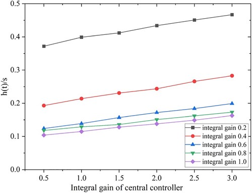
Table 3. Delay upper bounds under different $K_p^P$ and $K_i^P$.

	$K_p^P$
$K_i^P$	0.5	1.0	1.5	2.0	2.5	3.0
0.2	0.372	0.399	0.412	0.434	0.451	0.467
0.4	0.193	0.214	0.231	0.244	0.266	0.283
0.6	0.124	0.139	0.157	0.172	0.184	0.199
0.8	0.118	0.129	0.136	0.151	0.162	0.173
1	0.104	0.115	0.128	0.138	0.149	0.163

Under constant delay and disturbance-free condition ($\mu =0$, $\overline{\alpha }=\overline{\text{β}}=0$), a comparison is made between the time-delay upper bound with Theorem 1 and the methods expressed in Zhang et al. (2017) and Shyam et al. (2021). The results are shown in Table 4, where it is evident that the time-delay upper bound obtained from Theorem 1 is higher than the other two methods.

Table 4. Delay upper bounds of two-terminal LVDC system under different methods.

		Methods				Methods
$K_p^P$	$K_i^P$	Theorem 3.1	Zhang et al. (2017)	$K_p^P$	$K_i^P$	Theorem 3.1	Shyam et al. (2021)
2.0	0.2	0.434	0.430	0.5	0.1	0.483	0.470
2.0	0.4	0.244	0.241	0.5	0.8	0.118	0.102
2.5	0.2	0.451	0.446	5.0	0.1	0.447	0.421
2.5	0.6	0.184	0.177	5.0	0.8	0.220	0.203
3.0	0.2	0.467	0.462	8.0	0.1	0.351	0.331
3.0	0.8	0.173	0.166	8.0	0.8	0.212	0.188

Under time-varying delay and disturbance condition ($\overline{\alpha }$, $\overline{\text{β}}$, $\mu \ne 0$), the time-delay upper bounds from Theorem 1 and the method from Zhang et al. (2017) are presented in Table 5, demonstrating the effectiveness of the method proposed in this paper.

Table 5. Delay upper bounds of two-terminal LVDC system under different methods for $\mu =0.5$.

		$\overline{\alpha }=0$, $\overline{\text{β}}=0.025$		$\overline{\alpha }=\overline{\text{β}}=0.025$
$K_p^P$	$K_i^P$	Theorem 3.1	Zhang et al. (2017)	Theorem 3.1	Zhang et al. (2017)
0.5	0.2	0.338	0.329	0.309	0.289
0.5	0.4	0.144	0.136	0.128	0.117
0.5	0.6	0.117	0.105	0.101	0.100
1	0.2	0.378	0.366	0.373	0.354
1	0.4	0.190	0.172	0.182	0.165
1	0.6	0.127	0.111	0.117	0.106

The accuracy of the theoretical results is validated by LVDC system simulation based on MATLAB/Simulink.

1. Constant time-delay: The power disturbance $K\mathrm{\Delta }{u}_{ds}$ in the system model (17) is set as the form of (18), where $\overline{Z}=0$, $\overline{X}=0.1I_n$, $\overline{\alpha }=0$, $\overline{\text{β}}=0.025$. When $K_p^P=0.5$, $K_i^P=0.2$, the maximum allowable time-delay for the system is $h=0.341s$. Under the conditions mentioned, the variation in the DC bus voltage of the system is illustrated in Figure 5. It can be observed that the DC bus voltage eventually converges to the rated value.

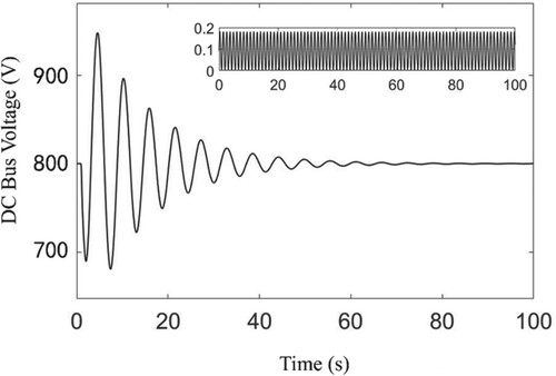
2. Time-varying delay: the DC bus voltage variation of the two-terminal LVDC system is shown in Figure 6 when considering variable time-delay and a given power disturbance condition, where $\overline{Z}=0$, $\overline{X}=0.1I_n$, $\overline{\alpha }=\overline{\text{β}}=0.025$. When $K_p^P=1.0$, $K_i^P=0.4$, the maximum allowable time-delay for the system is $h=0.182s$. $h\left(t\right)=0.182/2\sin \left(1/0.182t\right)+0.182/2$ is selected as a time-varying delay. The variation in the DC bus voltage of the system is illustrated in Figure 6. It can be observed the system gradually converges to the rated value.

Figure 5. Bus voltage response curve of two terminal LVDC system under the influence of constant time-delay.

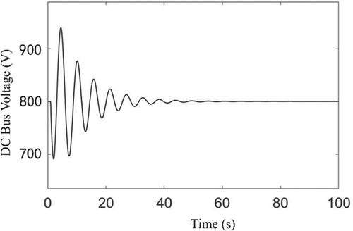
Figure 6. Bus voltage response curve of two terminal LVDC system under the influence of time-varying delay.

5. Conclusion

The stability of LVDC system under time-varying delays is investigated in this paper, and a hierarchical control model for LVDC system considering communication delays is constructed. By incorporating multiple integral terms and delay-dependent matrices, a novel Lyapunov-Krasovskii functional is constructed. In handling the functional derivatives, a combination of quadratic function inequalities and composite relaxation integral inequalities is used to obtain less conservative stability criteria. Finally, the effectiveness of the proposed method is validated through simulation results. Our future studies will focus on the stability analysis of multi time-delay LVDC system and the influence of uncertainty factors on the stability of the system during the modelling process.

Disclosure statement

No potential conflict of interest was reported by the author(s).

Appendix

In the following equation, $\mathrm{\Delta }$ is the small variation of variables near the steady-state operating point, the subscript ‘0’ represents the steady-state value of the variable, and the subscript ‘ref’ indicates the reference value of the variable.

The small-signal model of the slave station $VS{C}^{\text{2}}$ on the AC side in the dq coordinate system can be expressed as follows. (A1) $\{\begin{array}{c}{L}_s{\displaystyle \frac{d\mathrm{\Delta }{i}_{sd}^{\text{2}}}{dt}}=-\mathrm{\Delta }{u}_{od}^{\text{2}}+\omega L_s\mathrm{\Delta }{i}_{sq}^{\text{2}}-R_s\mathrm{\Delta }{i}_{sd}^{\text{2}}\\ L_s{\displaystyle \frac{d\mathrm{\Delta }{i}_{sq}^{\text{2}}}{dt}}=-\mathrm{\Delta }{u}_{oq}^{\text{2}}-\omega L_s\mathrm{\Delta }{i}_{sd}^{\text{2}}-R_s\mathrm{\Delta }{i}_{sq}^{\text{2}}\end{array}$(A1) The small-signal model of the DC-side capacitance node $VS{C}^2$ can be expressed as: (A2) $C_{\text{2}}{\displaystyle \frac{d\mathrm{\Delta }{u}_{dc}^{\text{2}}}{dt}}=-{\displaystyle \frac{\mathrm{\Delta }{P}_{dc}^{\text{2}}}{u_{dc,0}^{\text{2}}}}+{\displaystyle \frac{P_{dc}^{\text{2}}\mathrm{\Delta }{u}_{dc}^{\text{2}}}{u_{dc,0}^2}}+\mathrm{\Delta }{i}^{\text{2}}$(A2) The $VS{C}^2$ in dq coordinate axis includes the small-signal model for active power, reactive power, and power transfer to the DC side, which can be expressed as: (A3) $\{\begin{array}{l}{P}^{\text{2}}=1.5u_{sd}^{\text{2}}{i}_{sd}^{\text{2}}\\ Q^{\text{2}}=-1.5u_{sd}^{\text{2}}{i}_{sd}^{\text{2}}\\ P_{dc}^{\text{2}}=1.5(u_{od}^{\text{2}}{i}_{sd}^{\text{2}}+u_{oq}^{\text{2}}{i}_{sq}^{\text{2}})\end{array}$(A3) The small-signal model for the outer-loop control of the slave station $VS{C}^2$ can be expressed as: (A4) $\begin{array}{rl}& \{\begin{array}{l}\mathrm{\Delta }{i}_{sd,ref}^{\text{2}}=K_{pP}(\mathrm{\Delta }{P}^{\text{2}\ast }-1.5u_{sd,0}^2\mathrm{\Delta }{i}_{sd}^2)+\mathrm{\Delta }{W}_P^{\text{2}}\\ \mathrm{\Delta }{i}_{sq,ref}^2=K_{pQ}(\mathrm{\Delta }{Q}^{\text{2}\ast }+1.5u_{sd,0}^2\mathrm{\Delta }{i}_{sq}^2)+\mathrm{\Delta }{W}_Q^{\text{2}}\end{array}\end{array}$(A4) (A5) $\begin{array}{rl}& \{\begin{array}{l}\mathrm{\Delta }{W}_P^2={\displaystyle \frac{K_{iP}}{s}}(\mathrm{\Delta }{P}^{2\ast }-1.5u_{sd,0}^2\mathrm{\Delta }{i}_{sd}^2)\\ \mathrm{\Delta }{W}_Q^2={\displaystyle \frac{K_{iQ}}{s}}(\mathrm{\Delta }{Q}^{2\ast }+1.5u_{sd,0}^2\mathrm{\Delta }{i}_{sq}^2)\end{array}\end{array}$(A5) Similarly, small-signal model for the inner-loop control of the slave station $VS{C}^2$ can also be expressed as: (A6) $\begin{array}{rl}& \{\begin{array}{l}\mathrm{\Delta }{u}_{od}^2=K_{pd}(\mathrm{\Delta }{i}_{sd}^2-\mathrm{\Delta }{i}_{sd,ref}^2)+\mathrm{\Delta }{W}_d^2+\omega L_s\mathrm{\Delta }{i}_{sq}^2\\ \mathrm{\Delta }{u}_{oq}^2=K_{pq}(\mathrm{\Delta }{i}_{sq}^2-\mathrm{\Delta }{i}_{sq,ref}^2)+\mathrm{\Delta }{W}_q^2+\omega L_s\mathrm{\Delta }{i}_{sd}^2\end{array}\end{array}$(A6) (A7) $\begin{array}{rl}& \{\begin{array}{l}\mathrm{\Delta }{W}_d^2={\displaystyle \frac{K_{id}}{s}}(\mathrm{\Delta }{i}_{sd}^2-\mathrm{\Delta }{i}_{sd,ref}^2)\\ \mathrm{\Delta }{W}_q^2={\displaystyle \frac{K_{iq}}{s}}(\mathrm{\Delta }{i}_{sq}^2-\mathrm{\Delta }{i}_{sq,ref}^2)\end{array}\end{array}$(A7) The central controller is comprised of PI controllers and can be expressed as: (A8) $\{\begin{array}{l}\mathrm{\Delta }{P}^{2\ast }=K_p^P{P}_{CE}+\mathrm{\Delta }{W}_P^{\ast }=\left(K_p^P+{\displaystyle \frac{K_i^P}{s}}\right)P_{CE}\\ \mathrm{\Delta }{Q}^{2\ast }=K_p^Q{Q}_{CE}+\mathrm{\Delta }{W}_Q^{\ast }=\left(K_p^Q+{\displaystyle \frac{K_i^Q}{s}}\right)Q_{CE}\end{array}$(A8) Integrating Equations (A1) to (A8), the complete small-signal model for the slave station $VS{C}^2$ under the master-slave control strategy can be expressed as: (A9) ${\displaystyle \frac{d{x}_n^2}{dt}}=A_n^2{x}_n^2+B_n^2\mathrm{\Delta }{u}_n^2$(A9) To facilitate the subsequent construction of the time-delay model for the LVDC system, the output control variables of the central controller, which are also the input control variables for $VS{C}^2$, are represented using system state variables. In other words, let $B_n^2\mathrm{\Delta }{u}_n^2=A_{dn}^2\mathrm{\Delta }{x}_n^2$, which allows the Equation (A9) A9 be transformed as follows: (A10) ${\displaystyle \frac{d{x}_n^2\left(t\right)}{dt}}=A_n^2{x}_n^2\left(t\right)+A_{dn}^2{x}_n^2\left(t\right)$(A10) where $A_n^2$ is the state matrices; $B_n^2$ is the input matrices; $x_n^2$ is the complete small-signal model of the slave station $VS{C}^2$ includes state variables in the following format: $x_n^2=[\mathrm{\Delta }{u}_{dc}^2\mathrm{\Delta }{i}_{sd}^2\mathrm{\Delta }{i}_{sq}^2\mathrm{\Delta }{W}_P^2\mathrm{\Delta }{W}_Q^2\mathrm{\Delta }{W}_d^2\mathrm{\Delta }{W}_q^2\mathrm{\Delta }{W}_P^{\ast }\mathrm{\Delta }{W}_Q^{\ast }{]}^T$, $\mathrm{\Delta }{u}_n^2$ is the input control variables in the following format: $\mathrm{\Delta }{u}_n^2=[\mathrm{\Delta }{P}^{2\ast }\mathrm{\Delta }{Q}^{2\ast }{]}^T$.

The construction method for the complete small-signal model of the master station $VS{C}^1$ is similar to that of the slave station $VS{C}^2$, and the specific process is not further elaborated. The complete small-signal model for the master station $VS{C}^1$ can be then expressed as: (A11) ${\displaystyle \frac{d{x}_m^1}{dt}}=A_m^1{x}_m^1$(A11) Where $x_m^1$ is the state matrix; is the complete small-signal model for the master station $VS{C}^1$ in the following format: $x_m^1=[\mathrm{\Delta }{u}_{dc}^1\mathrm{\Delta }{i}_{sd}^1\mathrm{\Delta }{i}_{sq}^1\mathrm{\Delta }{W}_{ud}^1\mathrm{\Delta }{W}_{uq}^1\mathrm{\Delta }{W}_d^1\mathrm{\Delta }{W}_q^1{]}^T$.

It should be noted that the role of the master station is to maintain the bus voltage stability within the LVDC system. Therefore, the voltage reference value is constant, and no input control variables exist.

The small-signal model of the system's DC network can be expressed as: (A12) $\{\begin{array}{l}{L}_1{\displaystyle \frac{d\mathrm{\Delta }{i}_1}{dt}}=\mathrm{\Delta }{u}_{dc}^1-R_1\mathrm{\Delta }{i}_1-\mathrm{\Delta }{u}_{dc}\\ L_2{\displaystyle \frac{d\mathrm{\Delta }{i}_2}{dt}}=\mathrm{\Delta }{u}_{dc}-R_2\mathrm{\Delta }{i}_2-\mathrm{\Delta }{u}_{dc}^2\\ C_0{\displaystyle \frac{d\mathrm{\Delta }{u}_{dc}}{dt}}=\mathrm{\Delta }{i}_1-\mathrm{\Delta }{i}_2-{\displaystyle \frac{\mathrm{\Delta }{P}_{eq}}{u_{dc,0}}}+{\displaystyle \frac{P_{eq,0}\mathrm{\Delta }{u}_{dc}}{u_{dc,0}^2}}\end{array}$(A12) The complete small-signal model of the system's DC network can be expressed as: (A13) ${\displaystyle \frac{d\mathrm{\Delta }{x}_g}{dt}}=A_g\mathrm{\Delta }{x}_g+B_g\mathrm{\Delta }{u}_g+B_{ds}\mathrm{\Delta }{u}_d$(A13) where $A_g$ is the state matrices; $B_g$ is the input matrices; $B_{ds}$ is the disturbance matrices; $x_g$ is the state variables in the following format: $x_g={\left[\begin{array}{ccc}\mathrm{\Delta }{u}_{dc}& \mathrm{\Delta }{i}_1& \mathrm{\Delta }{i}_2\end{array}\right]}^T$, $\mathrm{\Delta }{u}_g$ is the input variables in the following format: $\mathrm{\Delta }{u}_g={\left[\begin{array}{cc}\mathrm{\Delta }{u}_{dc}^1& \mathrm{\Delta }{u}_{dc}^2\end{array}\right]}^T$, $\mathrm{\Delta }{u}_d$ is the equivalent aggregated load power in the following format: $\mathrm{\Delta }{u}_d=\left[\mathrm{\Delta }{P}_{eq}\right]$.

Since the DC-side voltages of both the master and slave stations are stably output under steady-state conditions, the $\mathrm{\Delta }{u}_{dc}^1$ and $\mathrm{\Delta }{u}_{dc}^2$ are both 0, (A13) can be further transformed as: (A14) ${\displaystyle \frac{d{x}_g\left(t\right)}{dt}}=A_g{x}_g\left(t\right)+B_{ds}\mathrm{\Delta }{u}_d\left(t\right)$(A14) Combining (A10), (A11), and (A14), the complete small-signal model of the LVDC system can be expressed as: (A15) ${\displaystyle \frac{dx\left(t\right)}{dt}}=A_{s}x\left(t\right)+A_{ds}x\left(t\right)+B_s\mathrm{\Delta }{u}_{ds}\left(t\right)$(A15)

References

- Castillo-Calzadilla, T., Cuesta, M. A., Olivares-Rodriguez, C., Macarulla, A. M., Legarda, J., & Borges, C. E. (2022). Is it feasible a massive deployment of low voltage direct current microgrids renewable-based? A technical and social sight. Renewable and Sustainable Energy Reviews, 161, 112198. https://doi.org/10.1016/j.rser.2022.112198
- Castro, L. M. (2022). Simulation framework for automatic load frequency control studies of VSC-based AC/DC power grids. International Journal of Electrical Power & Energy Systems, 141, 108187. https://doi.org/10.1016/j.ijepes.2022.108187
- Chen, G., & Zhao, Z. (2018). Delay effects on consensus-based distributed economic dispatch algorithm in microgrid. IEEE Transactions on Power Systems, 33(1), 602–612. https://doi.org/10.1109/TPWRS.2017.2702179
- Chia, Y. Y., Lee, L. H., Shafiabady, N., & Isa, D. (2015). A load predictive energy management system for supercapacitor-battery hybrid energy storage system in solar application using the Support Vector Machine. Applied Energy, 137, 588–602. https://doi.org/10.1016/j.apenergy.2014.09.026
- Coelho, E. A., Wu, D., Guerrero, J. M., Vasquez, J. C., Dragicˇević, T., Stefanović, C., & Popovski, P. (2016). Small-signal analysis of the microgrid secondary control considering a communication time delay. IEEE Transactions on Industrial Electronics, 63(10), 6257–6269. https://doi.org/10.1109/TIE.2016.2581155
- Deng, W., Pei, W., & Li, L. (2018). Active stabilization control of multi-terminal AC/DC hybrid system based on flexible low-voltage DC power distribution. Energies, 11(3), 502. https://doi.org/10.3390/en11030502
- Deng, W., Pei, W., Wu, Q., & Zhuang, Y. (2022). Analysis of interactive behavior and stability of low-voltage multiterminal DC System under droop control modes. IEEE Transactions on Industrial Electronics, 69(7), 6948–6959. https://doi.org/10.1109/TIE.2021.3095803
- Deng, W., Pei, W., Wu, Q., Zhuang, Y., & Li, Y. (2023). An improved additional control method for extending stable operating region of multi-terminal LVDC system. IEEE Transactions on Smart Grid. doi:10.1109/TSG.2023.3307930
- Du, W., Zhang, J., Zhang, Y., & Qian, Z. (2013). Stability criterion for cascaded system with constant power load. IEEE Transactions on Power Electronics, 28(4), 1843–1851. https://doi.org/10.1109/TPEL.2012.2211619
- Gerber, D. L., Ghatpande, O. A., & Nazir, M. (2022). Energy and power quality measurement for electrical distribution in AC and DC microgrid buildings. Applied Energy, 308, 118308. https://doi.org/10.1016/j.apenergy.2021.118308
- Hallemans, L., Ravyts, S., & Govaerts, G. (2022). A stepwise methodology for the design and evaluation of protection strategies in LVDC microgrids. Applied Energy, 310, 118420. https://doi.org/10.1016/j.apenergy.2021.118420
- Heydari, R., Dragicevic, T., & Blaabjerg, F. (2019). High-bandwidth secondary voltage and frequency control of VSC-based AC microgrid. IEEE Transactions on Power Electronics, 34(11), 11320–11331. https://doi.org/10.1109/TPEL.2019.2896955
- Hong, J. S., Ha, J. I., Cui, S., & Hu, J. (2023). Topology and control of an enhanced dual-active bridge converter with inherent bipolar operation capability for LVDC distribution systems. IEEE Transactions on Power Electronics, 38(10), 12774–12789. https://doi.org/10.1109/TPEL.2023.3297389
- Hussain, M. N., Mishra, R., & Agarwal, V. (2018). A frequency-dependent virtual impedance for voltage-regulating converters feeding constant power loads in a DC microgrid. IEEE Transactions on Industry Applications, 54(6), 5630–5639. https://doi.org/10.1109/TIA.2018.2846637
- Lin, W., He, Y., Zhang, C., Wu, M., & Shen, J. (2019). Extended dissipativity analysis for Markovian jump neural networks with time-varying delay via delay-product-type functionals. IEEE Transactions on Neural Networks and Learning Systems, 30(8), 2528–2537. https://doi.org/10.1109/TNNLS.2018.2885115
- Liu, Y., Deng, W., Yang, P., Teng, Y., Zhang, X., Yang, Y., & Pei, W. (2023). Dispatchable droop control strategy for DC microgrid. Energy Reports, 9, 98–102. https://doi.org/10.1016/j.egyr.2023.09.158
- Long, F., Jiang, L., He, Y., & Wu, M. (2019). Stability analysis of systems with time-varying delay via novel augmented Lyapunov–Krasovskii functionals and an improved integral inequality. Applied Mathematics and Computation, 357, 325–337. https://doi.org/10.1016/j.amc.2019.04.004
- Luo, H., & Hu, Z. C. (2022). Stability analysis of sampled-data load frequency control systems with multiple delays. IEEE Transactions on Control Systems Technology, 30(1), 434–442. https://doi.org/10.1109/TCST.2021.3061556
- Lv, Z., Zhou, M., Wang, Q., & Hu, W. (2021). Small-signal stability analysis for multi-terminal LVDC distribution network based on distributed secondary control strategy. Electronics, 10(13), 1575. https://doi.org/10.3390/electronics10131575
- Magne, P., Nahid-Mobarakeh, B., & Pierfederici, S. (2012). General active global stabilization of multiloads DC-power networks. IEEE Transactions on Power Electronics, 27(4), 1788–1798. https://doi.org/10.1109/TPEL.2011.2168426
- Miranda, R. F., Salgado-Herrera, N. M., Rodríguez-Hernández, O., Rodríguez-Rodríguez, J. R., Robles, M., Ruiz-Robles, D., & Venegas-Rebollar, V. (2022). Distributed generation in low-voltage DC systems by wind energy in the Baja California Peninsula, Mexico. Energy, 242, 122530. https://doi.org/10.1016/j.energy.2021.122530
- Peyghami, S., Davari, P., Mokhtari, H., & Blaabjerg, F. (2019). Decentralized droop control in DC microgrids based on a frequency injection approach. IEEE Transactions on Smart Grid, 10(6), 6782–6791. https://doi.org/10.1109/TSG.2019.2911213
- Purgat, P., Shekhar, A., Qin, Z., & Bauer, P. (2023). Low-voltage dc system building blocks: Integrated power flow control and short circuit protection. IEEE Industrial Electronics Magazine, 17(1), 6–20. https://doi.org/10.1109/MIE.2021.3106275
- Qian, W., Li, Y., Chen, Y., & Liu, W. (2020). L2-L∞ filtering for stochastic delayed systems with randomly occurring nonlinearities and sensor saturation. International Journal of Systems Science, 51(13), 2360–2377. https://doi.org/10.1080/00207721.2020.1794080
- Qian, W., Lu, D., Guo, S., & Zhao, Y. (2022). Distributed state estimation for mixed delays system over sensor networks with multichannel random attacks and Markov switching topology. IEEE Transactions on Neural Networks and Learning Systems, https://doi.org/10.1109/TNNLS.2022.3230978
- Qian, W., Xing, W., & Fei, S. (2021). H∞ state estimation for neural networks with general activation function and mixed time-varying delays. IEEE Transactions on Neural Networks and Learning Systems, 32(9), 3909–3918. https://doi.org/10.1109/TNNLS.2020.3016120
- Seo, H. C., Gwon, G. H., & Park, K. W. (2023). New protection method considering fault section in LVDC distribution system with PV system. Journal of Electrical Engineering & Technology, 18(1), 239–248. https://doi.org/10.1007/s42835-022-01224-x
- Seuret, A., & Gouaisbaut, F. (2018). Stability of linear systems with time-varying delays using Bessel–Legendre inequalities. IEEE Transactions on Automatic Control, 63(1), 225–232. https://doi.org/10.1109/TAC.2017.2730485
- Shyam, A. B., Anand, S., & Sahoo, S. R. (2021). Effect of communication delay on consensus-based secondary controllers in DC microgrid. IEEE Transactions on Industrial Electronics, 68(4), 3202–3212. https://doi.org/10.1109/TIE.2020.2978719
- Tian, Y., & Wang, Z. (2021). Composite slack-matrix-based integral inequality and its application to stability analysis of time-delay systems. Applied Mathematics Letters, 120, 107252. https://doi.org/10.1016/j.aml.2021.107252
- Vafamand, N., Khooban, M. H., Dragičević, T., Boudjadar, J., & Asemani, M. H. (2019). Time-delayed stabilizing secondary load frequency control of shipboard microgrids. IEEE Systems Journal, 13(3), 3233–3241. https://doi.org/10.1109/JSYST.2019.2892528
- Xiong, L., Li, H., & Wang, J. (2018). LMI based robust load frequency control for time delayed power system via delay margin estimation. International Journal of Electrical Power & Energy Systems, 100, 91–103. https://doi.org/10.1016/j.ijepes.2018.02.027
- Zeng, H. B., Lin, H. C., He, Y., Zhang, C. K., & Teo, K. L. (2020). Improved negativity condition for a quadratic function and its application to systems with time-varying delay. IET Control Theory & Applications, 14(18), 2989–2993. https://doi.org/10.1049/iet-cta.2019.1464
- Zeng, H. B., Liu, X. G., & Wang, W. (2019). A generalized free-matrix-based integral inequality for stability analysis of time-varying delay systems. Applied Mathematics and Computation, 354, 1–8. https://doi.org/10.1016/j.amc.2019.02.009
- Zhang, C., Wang, H., Wang, Z., & Li, Y. (2023). Active detection fault diagnosis and fault location technology for LVDC distribution networks. International Journal of Electrical Power & Energy Systems, 148, 108921. https://doi.org/10.1016/j.ijepes.2022.108921
- Zhang, C.-K., He, Y., Jiang, L., & Wu, M. (2017). Notes on stability of time-delay systems: Bounding inequalities and augmented Lyapunov-Krasovskii functionals. IEEE Transactions on Automatic Control, 62(10), 5331–5336. https://doi.org/10.1109/TAC.2016.2635381
- Zhang, L., Chen, K., Lyu, L., & Cai, G. (2019). Research on the operation control strategy of a low-voltage direct current microgrid based on a disturbance observer and neural network adaptive control algorithm. Energies, 12(6), 1162. https://doi.org/10.3390/en12061162
- Zhao, D., Jiang, S., Hu, D., Wang, Y., Jin, X., & Sun, C. (2022). Summary and prospect of technology development of MVDC and LVDC distribution technology. In 2022 IEEE 5th International Electrical and Energy Conference (CIEEC) (pp. 1294–1300). Institute of Electrical and Electronics Engineers. https://doi.org/10.1109/CIEEC54735.2022.9845945
Appendix
In the following equation, is the small variation of variables near the steady-state operating point, the subscript ‘0’ represents the steady-state value of the variable, and the subscript ‘ref’ indicates the reference value of the variable.
The small-signal model of the slave station on the AC side in the dq coordinate system can be expressed as follows.
(A1)
(A1) The small-signal model of the DC-side capacitance node
can be expressed as:
(A2)
(A2) The
in dq coordinate axis includes the small-signal model for active power, reactive power, and power transfer to the DC side, which can be expressed as:
(A3)
(A3) The small-signal model for the outer-loop control of the slave station
(A4)
(A5)
(A5) Similarly, small-signal model for the inner-loop control of the slave station
can also be expressed as:
(A6)
(A7)
(A7) The central controller is comprised of PI controllers and can be expressed as:
(A8)
(A8) Integrating Equations (A1) to (A8), the complete small-signal model for the slave station
under the master-slave control strategy can be expressed as:
(A9)
(A9) To facilitate the subsequent construction of the time-delay model for the LVDC system, the output control variables of the central controller, which are also the input control variables for
, are represented using system state variables. In other words, let
, which allows the Equation (A9) A9 be transformed as follows:
(A10)
(A10) where
is the state matrices;
is the input matrices;
is the complete small-signal model of the slave station
includes state variables in the following format:
,
is the input control variables in the following format: