Sensitivity analysis of the physics options in the Weather Research and Forecasting model for typhoon forecasting in Japan and its impacts on storm surge simulations

ABSTRACT

Weather Research and Forecasting (WRF) model is useful for forecasting typhoons as an external force of storm surge forecasts. This study examines the variation in typhoon forecasts caused by different choices of arbitrary physics options in WRF and their influence on storm surge forecasts. Eight frequently used combinations of cloud microphysics and planetary boundary layers were extracted via a review of previous studies. Subsequently, sensitivity analyses of these physics options were performed, targeting nine typhoons that landed in Japan during 2015–2019.  Additionally, we conducted case studies of storm surge ensemble forecasts in Tokyo Bay and Osaka Bay using WRF-simulated typhoons generated in the sensitivity analysis. As a result, the ensemble mean of the forecasts was comparable to the storm surge reanalysis simulation results obtained using an empirical typhoon model wherein the best track data is integrated to reproduce atmospheric fields. This may be attributed to the fact that the typhoon parameters (intensity, size, approaching angle, and velocity) obtained from the best track at landfall were generally within the range of the parameters that were simulated using WRF.

KEYWORDS:

• Typhoon forecast
• WRF
• physics options
• sensitivity analysis
• ensemble storm surge forecast

1. Introduction

Tropical cyclones (typhoons) and storm surges have caused considerable damage in coastal areas around the world. The three-dimensional dynamical model (3D model) is frequently used for real-time typhoon forecast to reduce the risks and damages caused by these disasters. Among the 3D models, the Weather Research and Forecasting model (WRF) (Skamarock et al. 2008) has been commonly used. WRF is an open-source model and has numerous users worldwide. Specifically, there are more than 30,000 users and 3,000 WRF-related publications globally (Powers et al. 2017).

When WRF is used for typhoon forecast, the setting of its computational conditions influences the results of the forecast significantly. Therefore, several sensitivity analyses of various computational conditions of WRF have been conducted. Specifically, three computational conditions influence the accuracy of typhoon forecasts significantly: horizontal and vertical grid resolutions (Fovell and Su 2007; Davis et al. 2008; Wu et al. 2019), initial and boundary conditions (Davis et al. 2008; Wannawong et al. 2018), and physics options for representing sub-grid scale physical processes such as cloud physics and planetary boundary layers (Chandrasekar and Balaji 2012; Zhang et al. 2017; Di et al. 2019).

A higher grid resolution can generally be expected to provide a better typhoon forecast accuracy, and analysis data with high accuracy should be used to determine initial and boundary conditions. Thus, the choice of computational conditions for grid resolution and initial and boundary conditions can be narrowed down to some extent by performing a sensitivity analysis for a specific region. However, the best combination of physics options of WRF is typhoon-specific and no perfect combination of physics options for arbitrary typhoons exists (Ming et al. 2012; Zhang et al. 2017). Thus, sensitivity analyses are required to identify a combination of physics option (among a large number of possible combinations of physics options) that provides the highest typhoon forecast accuracy.

In WRF-ARW v.3.8.1, there are more than 9 million combinations of physics options (22 microphysics (MP), 12 planetary boundary layers (PBL), 7 surface-layer options, 13 cumulus parameterization (CU), 7 land surface options, 8 long wave radiation options, and 8 short wave radiation options). Generally, MP and PBL strongly affect the typhoon forecast accuracy, and there are 264 possible combinations (22 MP and 12 PBL) even if other options are fixed. This makes it unrealistic to analyze their sensitivity for all combinations of physics options considering all typhoons in the past. Therefore, the behavior of the WRF physics options for each typhoon is not completely known, which causes uncertainty in the typhoon forecasts.

For storm surge forecast, some studies use typhoon forecast results of WRF as an external force (Douluri et al. 2017; Musinguzi et al. 2019; Jang et al. 2020; Tsai et al. 2020). Because the accuracy of typhoon forecast affects the accuracy of storm surge forecast, the improvement in the accuracy of typhoon forecast should result in a corresponding increase in the accuracy of storm surge forecast. Moreover, several studies have investigated the magnitude of variation in the storm surge forecast with respect to the variation in each typhoon parameter (e.g. intensity, size, velocity, and approaching angle) by adopting the best tracks by changing one of the typhoon parameters, while others were fixed (Li et al. 2019). However, these studies used parametric (empirical) typhoon models. Few studies (e.g. Valle, Curchitser, and Bruyere 2020) have investigated the extent to which storm surges vary due to uncertainty in the parameters of typhoons simulated by 3D models such as WRF.

This study investigates the variation in typhoon forecasts, including the highly arbitrary parameters associated with the selection of WRF physics options that affect the forecast accuracy considerably. Additionally, the influence of the variability in typhoon forecasts on the variability in storm surge forecasts is quantitatively investigated. First, we conduct sensitivity analyses of the physics options of WRF for typhoons that had made landfall in Japan, which have not been studied extensively to date. The sensitivity analyses focus on the typhoons and combinations of physics options that improve the forecast accuracy of typhoons. Subsequently, ensemble forecasts of storm surges are conducted to account for the uncertainty in the predicted storm surge associated with the choice of physics options of WRF. Finally, we verify the accuracy of the storm surge forecast results and summarize the future works.

2. Method

2.1. Summary of target typhoons

Target typhoons for this study and their characteristics (typhoon parameters) are listed in Table 1. We selected nine typhoons that landed in Japan during 2015–2019, as shown in Table 2. Although all typhoons in the past should have been considered, owing to limited computational resources, only nine typhoons were selected for this study. The typhoons were selected objectively to ensure that they evenly cover the following typhoon parameters: 1) location of occurrence of the typhoon (latitude and longitude); 2) minimum central pressure of the typhoon; 3) mean typhoon velocity; 4) month of occurrence; 5) maximum diameter of strong wind (the area with 10-min averaged maximum wind speed ≧ 15 m/s); and 6) maximum diameter of storm wind (where 10-min averaged maximum winds ≧ 25 m/s). Figure 1 shows the distribution map of the abovementioned typhoon parameters. The initial condition of WRF was determined using the final operational global analysis data from the Global Forecasting System of the National Centers for Environmental Prediction (hereafter referred to as NCEP-FNL) (ds083.3). The NCEP-FNL has a horizontal resolution of 0.25 (deg) and is based on a large number of observations than the NCEP Global Forecast System (NCEP-GFS). NCEP-FNL was launched in July 2015; therefore, the typhoons that landed after this year were selected for this study. The typhoon tracks of all the selected typhoons provided by the Japan Meteorological Agency (JMA) best tracks (BT) are shown in Figure 2.

Figure 1. All 24 typhoons that caused landfall in Japan during 2015 − 2019, organized by the typhoon occurrence location, the intensity, the mean velocity, the occurrence month, the maximum diameter of strong wind, and the maximum diameter of storm wind. The markers indicate to which class each of the nine typhoons considered in this study belongs. Max. diameter of storm wind area indicates the diameter of the area with 10 min averaged maximum wind speed ≥ 25 m/s and Max. diameter of strong wind area is the same but with 15 m/s of maximum wind speed.

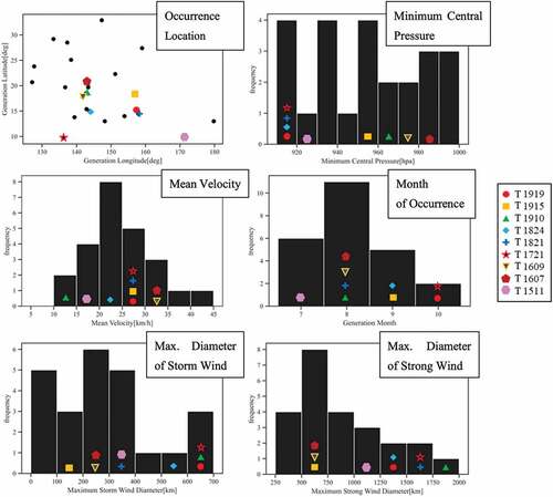
Figure 2. (a) Best tracks of the nine typhoons under consideration in this study. The red box in the figure is the computational domain of the WRF. (b) Best tracks of all 24 typhoons that caused landfall in Japan from 2015 to 2019. The gray line shows the track of the typhoons not considered in this study. Notably, T1915 means typhoon no. 15 in 2019.

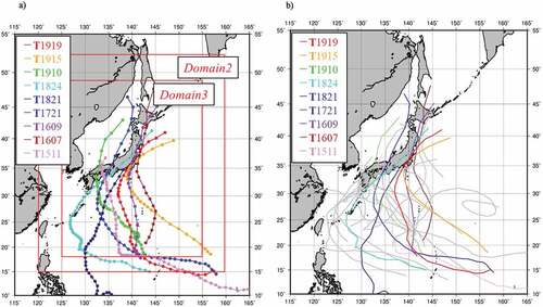
Table 1. Typhoon data analyzed in this study. These typhoon data are the JMA’s best tracks obtained from digital typhoons. T1511 means typhoon No. 11 in 2015. Lifespan is the time between the onset of a typhoon and its disappearance as an extratropical cyclone. The strong wind area is the area around a typhoon where winds with an average wind speed of 15 m/s or higher may blow where there is no influence of topography or other factors. Usually, the area is indicated using a circle. The storm wind area is the same but with an average wind speed of 25 m/s.

Typhoon (YYNN)	Minimum central pressure (hPa)	Maximum sustained wind speed (m/s)	Maximum diameter of the storm wind circle (km)	Maximum diameter of the strong wind circle (km)	Mean velocity (km/h)
T1919	915	54	650	1400	27
T1915	955	43.7	190	560	29.1
T1910	965	38.6	670	1800	14.2
T1824	915	54	500	1300	20.9
T1821	915	54	370	1500	27.9
T1721	915	51.4	610	1700	22.5
T1609	975	33.4	220	500	34.6
T1607	980	28.3	260	610	32.7
T1511	920	51.4	370	1200	18
Typhoon (YYNN)	Occurrence latitude (deg.)	Occurrence longitude (deg.)	Occurrence date	Lifespan (h)
T1919	15.1	157.4	Oct. 5th, 2019	177
T1915	18.6	156.7	Sep. 4th, 2019	126
T1910	18.5	142.8	Aug. 6th, 2019	246
T1824	15	143.7	Sep. 21st, 2018	234
T1821	14.5	157.9	Aug. 27th, 2018	198
T1721	9.7	136.2	Oct. 15th, 2017	174
T1609	17.8	141.8	Aug. 19th, 2016	93
T1607	20.9	142.9	Aug. 13th, 2016	96
T1511	9.8	170.8	July 17th, 2015	330

Table 2. Case name and initial conditions of typhoons. Here, T1915 is the abbreviation of typhoon no. 15 in 2019, the same as in Table 1. “Initialization time” represents the forecast start time, and columns 4 and 5 show the time and distance to the landfall at the start of the typhoon forecast, respectively.

Typhoon no. (YYNN)	Initialization time (UTC)	Case name (YYNNDDHH)	Hours to landfall (h) (at initialization time)	Distance to landfall point (km) (at initialization time)
T1919	October 8, 12:00	19190812	93	1430
	October 9, 12:00	19190912	69	1137
	October 10, 12:00	19191012	45	785
	October 11, 12:00	19191112	21	435
T1915	September 6, 0:00	19150600	67	1823
	September 7, 0:00	19150700	43	959
T1910	August 12, 12:00	19101212	66	745
	August 13, 0:00	19101300	54	513
	August 13, 12:00	19101312	42	410
T1824	September 26, 0:00	18242600	95	1201
	September 27, 0:00	18242700	71	1142
	September 28, 0:00	18242800	47	1165
T1821	August 31, 0:00	18213100	99	1703
	September 1, 0:00	18210100	75	1237
	September 2, 0:00	18210200	51	849
T1721	October 20, 0:00	17212000	66	1935
	October 21, 0:00	17212100	42	1290
T1609	August 20, 0:00	16092000	51	1617
T1607	August 14, 0:00	16071400	56	1501
T1511	July 14, 0:00	15111400	62	1195
	July 15, 0:00	15111500	38	778

2.2. Methods of sensitivity analyses for WRF physics options

In this study, four MPs and two PBLs were analyzed; other physics options were fixed. It is difficult to consider all physics options even for MP and PBL. Therefore, we focused on options that have been commonly used in previous studies (Table 3). The previous studies listed in Table 3, which were surveyed by the authors, perform comprehensive sensitivity analyses of WRF to MP and PBL, especially those focusing on the typhoon track and intensity. It should be noted, however, that not all the related literature is necessarily covered. For MP, the following schemes are often used (Figure 3(a)); Purdue Lin scheme (Chen and Sun 2002, hereafter LIN), WSM3 (WRF Single-Moment 3-class scheme, Hong, Jimy, and Chen 2004), WSM5 (WRF Single-Moment 5-class scheme, Hong, Jimy, and Chen 2004), Ferrier Eta scheme, WSM6 (WRF Single-Moment 6-class scheme, Hong and Lim 2006), and THOMP (Thompson et al. 2008). Notably, Di et al. (2019) suggested that WSM5 and THOMP provide the best forecast performance of minimum central pressure and track (respectively) for 15 typhoons that occurred from 2011 to 2015 in the Western Pacific Ocean, similar to the area we considered. Additionally, Park et al. (2020) discovered that, with WSM3, the typhoon intensity was underestimated owing to lower latent heat release compared to WSM5 and WSM6. Thus, they suggested that advanced cloud microphysics schemes, such as WSM5 and WSM6, will improve the intensity forecast of typhoons moving into the mid-latitudes. In addition to WSM6 (which is the most frequently used) and LIN (which is the second most frequently used), WSM5 and THOMP were adopted in this study, although WSM3 and Ferrier Eta were used more often than WSM5 and THOMP in previous studies. LIN is a six-class scheme that is the basis of several bulk cloud microphysics schemes, and the WSM5 is a five-class scheme that does not consider graupel. WSM6 is a six-class scheme that considers graupel, based on WSM5. THOMP is a partially double-moment scheme, i.e. in addition to the mixing ratio, the number concentration of ice and rain is predicted in this scheme. For PBL, the Yonsei University scheme (Hong, Yign, and Jimy 2006, hereafter YSU) is often used because YSU performs the best in forecasting the track and intensity of typhoons, as reported by several studies (Osuri et al. 2012; Srinivas et al. 2013; Wannawong et al. 2018; Wu et al. 2019). However, because there are some cases where the accuracy of the Mellor-Yamada-Janjic Scheme (Janjic 1994; Mesinger 1993, hereafter MYJ) outperforms that of the YSU (Chandrasekar and Balaji 2012; Mau and Min, 2017), these two options were tested in the sensitivity test. YSU is a first-order closure and a non-local scheme. Conversely, MYJ is a 1.5-order closure local scheme with an equation for prognosis of turbulent kinetic energy (TKE). Notably, although it would be preferable to consider all available physics options, we only considered eight combinations because of computational resource constraints. Table 4 shows the WRF configurations, and Table 5 shows the physics options that are analyzed in this study. For WRF domain, global forecast was performed (domain 1) by WRF. In a study by Bopape et al. (2021), the less accurate global analysis data were used in the WRF boundary conditions, which significantly affected the child domain, resulting in low accuracy of typhoon forecast. One of the solutions to this problem is to use lateral boundary conditions by WRF (conduct WRF global run to make lateral boundary conditions of child domain of WRF) to guarantee physical consistencies in all WRF domains. Although the method of global forecast in WRF has been used in few typhoon-related studies, we adopted the global forecast method because we confirmed in preliminary experiments (not shown here) that the adequate level (comparable to other major meteorological data NCEP-FNL (ds083.3), NCEP-GFS (ds084.1), and JMA Meso-Scale Model (JMA-MSM)) of typhoon forecast accuracy could be obtained in WRF global simulation. Some studies also show that the accuracy of typhoon forecast using WRF global forecast as lateral boundary conditions is sufficient (Shirai et al. 2020).

Figure 3. Physics options commonly used in existing sensitivity analysis studies. (a): For cloud microphysics (MP), and (b): for planetary boundary layer (PBL). 32 studies on physics-option-sensitivity analysis and tropical cyclone forecast experiment using WRF published from 2007 to 2020 are tabulated (for more detail, see Table 3). Option names and order are the same as those in Table 3.

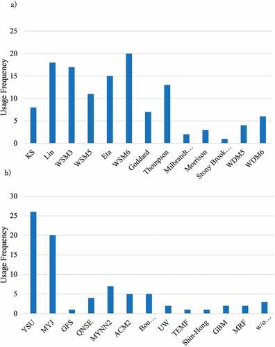
Table 3. Physics options used in sensitivity analysis studies using WRF that conduct typhoon forecasts. The references, and the horizontal resolution of WRF in the paper are also listed. Option is the name of the physics option that can be selected in WRF, and Option No. in WRF is the number of the physics option to be listed in the namelist.input of WRF. The marks (◯, ◎, ◆, ★) denote, respectively, ◯: used in the study, ◎: the best accuracy in forecasting the typhoon intensity, ◆: the best accuracy in forecasting the typhoon track, and ★: the best accuracy in both track and intensity. For the “highest accuracy” criterion, typhoon tracks are defined as cases where the errors are on average small throughout the entire time series (evaluated by some indices such as track error) or where the paper mentions the highest accuracy in track forecasts when no accuracy evaluation by some indices is conducted. For typhoon intensity, if statistical indices such as ME were used to evaluate the forecasting accuracy, the case with the smallest “error” is judged as the highest accuracy case. If no indices are used to evaluate the intensity forecasting accuracy, the authors judged the case in which the maximum wind speed and/or minimum central pressure values at the time of the strongest typhoon intensity are closest to the observed values, and the accuracy is the highest.

				Cloud microphysics (MP)													Planetary boundary layer (PBL)
			Option	KS	Lin	WSM3	WSM5	Eta	WSM6	Goddard	Thompson	Milbrandt-Yau	Morrison	Stony Brook Univ	WDM5	WDM6	YSU	MYJ	GFS	QNSE	MYNN2	ACM2	BouLac	UW	TEMF	Shin-Hong	GBM	MRF	w/o PBL
			Option no. in WRF	1	2	3	4	5	6	7	8	9	10	13	14	16	1	2	3	4	5	7	8	9	10	11	12	99	-
	References	Tropical cyclone(s)	Horizontal resolution (km)
1	Fovell and Su (2007)	Hurricane Rita	30, 12	〇	〇	〇
2	Li and Pu (2008)	Hurricane Emily	3	◎	〇	〇	〇	◆	〇								〇	◎
3	Li and Pu (2009)	Hurricane Emily	9, 3		〇												◆	◎
4	Hill and Lackmann (2009)	Idealized	36,12,4														〇	〇
5	Nolan et al. (2009)	Hurricane Isabel	0.44														〇	〇
6	Tao et al. (2011)	Hurricane Katlina	1.667	〇	〇	〇	〇	〇	〇									〇
7	Osuri et al. (2012)	9 Cyc.s during 2005–2008	27			〇											★	〇
8	Chandrasekar and Balaji (2012)	Cyclone Jal	10	◆	〇	◎	〇	〇	〇	〇	〇		〇		〇	〇	〇	◎		〇	◆	〇	〇
9	Ming et al. (2012)	Typhoon Saomai	1.5		〇				〇	〇	〇		〇					〇
10	Nasrollahi et al. (2012)	Hurricane Rita	4	◆	◆	〇	〇	〇									〇
11	Srinvas et al. (2013)	21 Cyc.s 2000–2011	9		★	〇			〇								★	〇
12	Kim et al. (2013)	Typhoon Maemi	1.33		〇	〇	〇	〇	〇	〇	〇	〇		〇	〇	〇	〇	〇		〇	〇	〇	〇	〇					〇
13	Reddy et al. (2014)	Cyclone Jal	3		〇			◆	〇		〇						〇
14	Kanase et al. (2015)	Cyclone Aila,Jal	6.6					〇	〇								◆	◎
15	Chen, Qian, and Peng (2015)	5 Typ.s during 2012	24		〇			◆	〇	〇							◆	〇			〇
16	Sun,Zhong, and Lu (2015)	Typhoon Megi	20		〇	◆			〇		〇							〇
17	Islam et al. (2015)	Typhoon Haiyan	5			〇			◆	〇	◆	〇					◆			◆	〇	〇	〇
18	Douluri and Annapurnaish (2016)	Cyclone Hudhud	3	〇	★	〇		〇	◎		〇						〇
19	Chan and Chan (2016)	6 Typ.s during 2013	4				〇	〇	〇
20	Kloetzke et al. (2016)	Cyclone Ita	1			〇		◎	〇								〇	〇			◎
21	Choudhury and Das (2017)	Cyc. Hudhud, Phailin Lehar	3		〇					★	◎						〇
22	Saikumar and Ramashri (2017)	Cyclone Laila	5	〇	〇	〇	〇				★						〇
23	Mau and Min (2017)	Cyclone Roanu	3		◎			〇	◆								〇	◆
24	Zhang et al. (2017)	Hurricane Arthur	1.33			〇	〇		〇							〇	〇	〇				〇
25	Saikumar and Ramashri (2018)	Cyclone Vardah	9	〇	〇	★	〇	〇	〇	〇	〇				〇	〇	〇
26	Tang et al. (2018)	Idealized	3					〇										〇	〇
27	Wannawong et al. (2018)	Typhoon Durian	5				◎		〇		〇						〇
28	Di et al. (2019)	15 typs during 2011–2015	12		◎	〇	◎		〇		◆		〇		〇	〇	〇	〇			〇	〇		★			〇
29	Alam (2020)	Cyclone Fani	9													〇	〇						〇		◎	〇	◆	〇	〇
30	Maldonado et al. (2020)	Hurricane Otto	3					〇									◆	〇										〇	〇
31	Park et al. (2020)	10 Typ.s during 2012–2018	2			〇			★								〇
32	Rajeswari et al. (2020)	5 Cyc.s during 2011–2016	3								〇						◎	〇		〇	〇		〇

Table 4. WRF configurations.

WRF-ARW ver. 3.8.1
Grid size (number of grids)	D1: 111 km (360 × 180) (Global) D2: 22 km (200 × 200) D3: 4.5 km (780 × 780)
Vertical layers	40 layers (top: 50 hPa)
Nesting	One-way nesting
Map projection	Latitude-Longitude
Time step	D1: 300s, D2: 90s, D3: 20s
Initial and boundary conditions	NCEP-FNL (ds083.3, 6-hourly, 0.25 °×0.25°) for initial conditions Lateral boundary conditions of domain 2 is given by WRF global run (the result of domain 1).
Physics options (fixed)	Cumulus Parameterization: Kain Fritsch (option 1) Short Wave/Long Wave Radiation: RRTMG (option 4) Land-Surface Option: Unified Noah Land Surface Model (option 2) Surface-Layer Option: PBL dependent Revised MM5 scheme (option 1) with YSU (option 1) Eta Similarity Scheme (option 2) with MYJ (option 2)

Table 5. Targeted physics options for this study and case name.

Case	Cloud microphysics	Planetary boundary layer
Case 1	Lin et al. scheme	Yonsei University scheme
Case 2	Lin et al. scheme	Mellor-Yamada-Janjic scheme
Case 3	WRF Single-Moment 5-class scheme	Yonsei University scheme
Case 4	WRF Single-Moment 5-class scheme	Mellor-Yamada-Janjic scheme
Case 5	WRF Single-Moment 6-class scheme	Yonsei University scheme
Case 6	WRF Single-Moment 6-class scheme	Mellor-Yamada-Janjic scheme
Case 7	Thompson et al. scheme	Yonsei University scheme
Case 8	Thompson et al. scheme	Mellor-Yamada-Janjic scheme

2.3. Storm surge forecast

For the storm surge forecast, the Storm Surge and Tsunami Simulator in Oceans and Coastal Areas (STOC), which adopts the finite difference method for spatial discretization, was used. STOC calculates seawater motion from offshore to coastal zones due to storm surges (Tomita and Kakinuma 2005). In this study, we adopted STOC multilevel model (STOC-ML), which assumes a hydrostatic state in the vertical direction. Therefore, storm surge is computed with a lower computational load than a full-3D model, making it suitable for a real-time forecast. The governing equations of STOC-ML are shown in Equations (1)(1) $\begin{array}{rl}& {\gamma }_v\frac{\mathrm{\partial }u}{\mathrm{\partial }t}+\frac{\mathrm{\partial }}{\mathrm{\partial }x}\left({\gamma }_{x}uu\right)+\frac{\mathrm{\partial }}{\mathrm{\partial }y}\left({\gamma }_{y}vu\right)+\frac{\mathrm{\partial }}{\mathrm{\partial }z}\left({\gamma }_{z}wu\right)-f_{0}v\\ & =-{\gamma }_v\frac{1}{\rho }\frac{\mathrm{\partial }p}{\mathrm{\partial }x}+\frac{\mathrm{\partial }}{\mathrm{\partial }x}\left({\gamma }_x{\nu }_{H}2\frac{\mathrm{\partial }u}{\mathrm{\partial }x}\right)+\frac{\mathrm{\partial }}{\mathrm{\partial }y}\left\{{\gamma }_y{\nu }_H\left(\frac{\mathrm{\partial }u}{\mathrm{\partial }y}+\frac{\mathrm{\partial }v}{\mathrm{\partial }x}\right)\right\}\text{break}+\frac{\mathrm{\partial }}{\mathrm{\partial }z}\left\{{\gamma }_z{\nu }_V\left(\frac{\mathrm{\partial }u}{\mathrm{\partial }z}+\frac{\mathrm{\partial }w}{\mathrm{\partial }x}\right)\right\}\end{array}$(1) –(7(7) ${\tau }_{bx}=\frac{\rho g{n}^2{u}_b\sqrt{u_b^2+v_b^2}}{h^{\frac{1}{3}}},{\tau }_{by}=\frac{\rho g{n}^2{v}_b\sqrt{u_b^2+v_b^2}}{h^{\frac{1}{3}}}$(7) ).

(1) $\begin{array}{rl}& {\gamma }_v\frac{\mathrm{\partial }u}{\mathrm{\partial }t}+\frac{\mathrm{\partial }}{\mathrm{\partial }x}\left({\gamma }_{x}uu\right)+\frac{\mathrm{\partial }}{\mathrm{\partial }y}\left({\gamma }_{y}vu\right)+\frac{\mathrm{\partial }}{\mathrm{\partial }z}\left({\gamma }_{z}wu\right)-f_{0}v\\ & =-{\gamma }_v\frac{1}{\rho }\frac{\mathrm{\partial }p}{\mathrm{\partial }x}+\frac{\mathrm{\partial }}{\mathrm{\partial }x}\left({\gamma }_x{\nu }_{H}2\frac{\mathrm{\partial }u}{\mathrm{\partial }x}\right)+\frac{\mathrm{\partial }}{\mathrm{\partial }y}\left\{{\gamma }_y{\nu }_H\left(\frac{\mathrm{\partial }u}{\mathrm{\partial }y}+\frac{\mathrm{\partial }v}{\mathrm{\partial }x}\right)\right\}\text{break}+\frac{\mathrm{\partial }}{\mathrm{\partial }z}\left\{{\gamma }_z{\nu }_V\left(\frac{\mathrm{\partial }u}{\mathrm{\partial }z}+\frac{\mathrm{\partial }w}{\mathrm{\partial }x}\right)\right\}\end{array}$(1)

(2) $\begin{array}{rl}& {\gamma }_v\frac{\mathrm{\partial }v}{\mathrm{\partial }t}+\frac{\mathrm{\partial }}{\mathrm{\partial }x}\left({\gamma }_{x}uv\right)+\frac{\mathrm{\partial }}{\mathrm{\partial }y}\left({\gamma }_{y}vv\right)+\frac{\mathrm{\partial }}{\mathrm{\partial }z}\left({\gamma }_{z}wv\right)+f_{0}u\\ & =-{\gamma }_v\frac{1}{\rho }\frac{\mathrm{\partial }p}{\mathrm{\partial }y}+\frac{\mathrm{\partial }}{\mathrm{\partial }x}\left\{{\gamma }_x{\nu }_H\left(\frac{\mathrm{\partial }v}{\mathrm{\partial }x}+\frac{\mathrm{\partial }u}{\mathrm{\partial }y}\right)\right\}+\frac{\mathrm{\partial }}{\mathrm{\partial }y}\left({\gamma }_y{\nu }_{H}2\frac{\mathrm{\partial }v}{\mathrm{\partial }y}\right)\text{break}+\\ & \frac{\mathrm{\partial }}{\mathrm{\partial }z}\left\{{\gamma }_z{\nu }_V\left(\frac{\mathrm{\partial }v}{\mathrm{\partial }z}+\frac{\mathrm{\partial }w}{\mathrm{\partial }y}\right)\right\}\end{array}$(2)

(3) $p\left(z\right)=p_{atm}-\rho g\left(\eta -z\right)$(3)

(4) $\frac{\mathrm{\partial }}{\mathrm{\partial }x}\left({\gamma }_{x}u\right)+\frac{\mathrm{\partial }}{\mathrm{\partial }y}\left({\gamma }_{y}v\right)+\frac{\mathrm{\partial }}{\mathrm{\partial }z}\left({\gamma }_{z}w\right)=0$(4)

(5) ${\gamma }_z\frac{\mathrm{\partial }\eta }{\mathrm{\partial }t}+\frac{\mathrm{\partial }}{\mathrm{\partial }x}{\int }_{-h}^{\eta }{\gamma }_{x}udz+\frac{\mathrm{\partial }}{\mathrm{\partial }y}{\int }_{-h}^{\eta }{\gamma }_{y}vdz=0$(5)

(6) ${\tau }_{sx}={\rho }_a{\gamma }_a^2{W}_x\sqrt{W_x^2+W_y^2},{\tau }_{sy}={\rho }_a{\gamma }_a^2{W}_y\sqrt{W_x^2+W_y^2}$(6)

(7) ${\tau }_{bx}=\frac{\rho g{n}^2{u}_b\sqrt{u_b^2+v_b^2}}{h^{\frac{1}{3}}},{\tau }_{by}=\frac{\rho g{n}^2{v}_b\sqrt{u_b^2+v_b^2}}{h^{\frac{1}{3}}}$(7)

Equations (1)(1) $\begin{array}{rl}& {\gamma }_v\frac{\mathrm{\partial }u}{\mathrm{\partial }t}+\frac{\mathrm{\partial }}{\mathrm{\partial }x}\left({\gamma }_{x}uu\right)+\frac{\mathrm{\partial }}{\mathrm{\partial }y}\left({\gamma }_{y}vu\right)+\frac{\mathrm{\partial }}{\mathrm{\partial }z}\left({\gamma }_{z}wu\right)-f_{0}v\\ & =-{\gamma }_v\frac{1}{\rho }\frac{\mathrm{\partial }p}{\mathrm{\partial }x}+\frac{\mathrm{\partial }}{\mathrm{\partial }x}\left({\gamma }_x{\nu }_{H}2\frac{\mathrm{\partial }u}{\mathrm{\partial }x}\right)+\frac{\mathrm{\partial }}{\mathrm{\partial }y}\left\{{\gamma }_y{\nu }_H\left(\frac{\mathrm{\partial }u}{\mathrm{\partial }y}+\frac{\mathrm{\partial }v}{\mathrm{\partial }x}\right)\right\}\text{break}+\frac{\mathrm{\partial }}{\mathrm{\partial }z}\left\{{\gamma }_z{\nu }_V\left(\frac{\mathrm{\partial }u}{\mathrm{\partial }z}+\frac{\mathrm{\partial }w}{\mathrm{\partial }x}\right)\right\}\end{array}$(1) and (2(2) $\begin{array}{rl}& {\gamma }_v\frac{\mathrm{\partial }v}{\mathrm{\partial }t}+\frac{\mathrm{\partial }}{\mathrm{\partial }x}\left({\gamma }_{x}uv\right)+\frac{\mathrm{\partial }}{\mathrm{\partial }y}\left({\gamma }_{y}vv\right)+\frac{\mathrm{\partial }}{\mathrm{\partial }z}\left({\gamma }_{z}wv\right)+f_{0}u\\ & =-{\gamma }_v\frac{1}{\rho }\frac{\mathrm{\partial }p}{\mathrm{\partial }y}+\frac{\mathrm{\partial }}{\mathrm{\partial }x}\left\{{\gamma }_x{\nu }_H\left(\frac{\mathrm{\partial }v}{\mathrm{\partial }x}+\frac{\mathrm{\partial }u}{\mathrm{\partial }y}\right)\right\}+\frac{\mathrm{\partial }}{\mathrm{\partial }y}\left({\gamma }_y{\nu }_{H}2\frac{\mathrm{\partial }v}{\mathrm{\partial }y}\right)\text{break}+\\ & \frac{\mathrm{\partial }}{\mathrm{\partial }z}\left\{{\gamma }_z{\nu }_V\left(\frac{\mathrm{\partial }v}{\mathrm{\partial }z}+\frac{\mathrm{\partial }w}{\mathrm{\partial }y}\right)\right\}\end{array}$(2) ) are momentum equations in x and y directions, respectively, where u, v, and w are the velocity components of the x, y, z directions of the Cartesian coordinate system, respectively, ${\gamma }_x,{\gamma }_y,{\gamma }_z$ (0 ≦ ${\gamma }_x,{\gamma }_y,{\gamma }_z$ ≦ 1.0) are the transmissivity rates in the x, y, and z directions, respectively, that represent the rate of liquid phase occupying the cross sections; ${\gamma }_v$ (0≦${\gamma }_v$≦1.0) is the effective volume rate, which is the rate of volume of liquid in a grid; $\rho$ is the density of water; $p$ denotes pressure; $f_0$ is the Coriolis parameter (because the Coriolis force is not considered in this study, $f_0=0$); and ${\nu }_H({\nu }_V$) is the vortex viscosity coefficient in the horizontal (vertical) direction. It should be noted that the vertical velocity w and the derivative terms in the z direction are always zero because the number of vertical layers is set to one in this study. Equation (3)(3) $p\left(z\right)=p_{atm}-\rho g\left(\eta -z\right)$(3) is the hydrostatic equation, where $p\left(z\right)$ is the pressure at any depth from the water surface, $p_{atm}$ is the atmospheric pressure; $g$ is the acceleration due to gravity, and $\eta$ is the water elevation at the sea surface. Equation (4)(4) $\frac{\mathrm{\partial }}{\mathrm{\partial }x}\left({\gamma }_{x}u\right)+\frac{\mathrm{\partial }}{\mathrm{\partial }y}\left({\gamma }_{y}v\right)+\frac{\mathrm{\partial }}{\mathrm{\partial }z}\left({\gamma }_{z}w\right)=0$(4) is the equation of continuity, and Equation (5)(5) ${\gamma }_z\frac{\mathrm{\partial }\eta }{\mathrm{\partial }t}+\frac{\mathrm{\partial }}{\mathrm{\partial }x}{\int }_{-h}^{\eta }{\gamma }_{x}udz+\frac{\mathrm{\partial }}{\mathrm{\partial }y}{\int }_{-h}^{\eta }{\gamma }_{y}vdz=0$(5) is an equation of free surface. Boundary conditions at the sea surface (Equation (6)(6) ${\tau }_{sx}={\rho }_a{\gamma }_a^2{W}_x\sqrt{W_x^2+W_y^2},{\tau }_{sy}={\rho }_a{\gamma }_a^2{W}_y\sqrt{W_x^2+W_y^2}$(6) ) and the sea bottom (Equation (7)(7) ${\tau }_{bx}=\frac{\rho g{n}^2{u}_b\sqrt{u_b^2+v_b^2}}{h^{\frac{1}{3}}},{\tau }_{by}=\frac{\rho g{n}^2{v}_b\sqrt{u_b^2+v_b^2}}{h^{\frac{1}{3}}}$(7) ) are also shown, where ${\rho }_a$ is the density of air, $W_x,W_y$ are the surface wind speeds in the x and y directions, respectively, that are used to calculate wind stress at the sea surface, ${\gamma }_a^2$ is a drag coefficient at the sea surface, which has a constant value $({\gamma }_a^2=0.001\times \left(1.29-0.024\sqrt{W_x^2+W_y^2}\right)\mathrm{i}\mathrm{f}\sqrt{W_x^2+W_y^2}\text{break}<8.0\mathrm{m}/\mathrm{s}$, ${\gamma }_a^2=0.001\times (0.581+0.063\sqrt{W_x^2+W_y^2}$ if $\sqrt{W_x^2+W_y^2}\ge 8.0\mathrm{m}/\mathrm{s}$); $u_b$ ($v_b)$ is the x(y) component of the seawater velocity at the sea bottom, and $h$ is the water depth from the datum level of the sea. In Equation (7)(7) ${\tau }_{bx}=\frac{\rho g{n}^2{u}_b\sqrt{u_b^2+v_b^2}}{h^{\frac{1}{3}}},{\tau }_{by}=\frac{\rho g{n}^2{v}_b\sqrt{u_b^2+v_b^2}}{h^{\frac{1}{3}}}$(7) , Manning’s formula is used to calculate the sea bottom stress ${\tau }_{bx},{\tau }_{by}$, where n is Manning’s roughness coefficient. The boundary condition for the outermost region is an open boundary condition. The surface (10 m above the surface) wind field and the mean sea-level pressure field that are the results of typhoon forecast using WRF are given hourly to STOC-ML. Domain 3 of WRF is interpolated into Domain 1–Domain 3 of STOC-ML. This interpolation process is necessary because the grids of the rectangular planar coordinate system of STOC-ML do not match with the latitude-longitude coordinate system of WRF. Data obtained from the General Bathymetric Chart of the Oceans (GEBCO) 30 arc-second global grid of elevations were adopted as the terrain data. Both the analyzed domain and tide-gauge stations that are used for validating storm surge forecast results are shown in Figure 4. The two target areas of storm surge forecasts in this study were the Tokyo and Osaka bays. Low-lying areas close to these bays are typically densely populated and are likely to be severely damaged by storm surge disasters. Table 6 shows the computational conditions of STOC-ML. For grid resolutions of storm surge simulations, some studies have used a grid size of up to 10–30 m (Valle et al. 2018; Jang et al. 2020). Conversely, in coastal areas, a grid size of several hundred meters to 1 km is often used (Douluri et al. 2017; Zhang et al. 2017; Torres et al. 2019). This is because the accuracy of the storm surge forecast is not necessarily improved by using a finer grid size although the computational time is increased (Lin et al. 2012; Honda, Naito, and Asai 2016). Therefore, to balance the accuracy of storm surge forecast and its computational cost, we adopted 270 m grid resolution for the finest domain (domain 3), similar to that used by Tsai et al. (2020). Additionally, in this study, two levels of nesting were adopted at 810 m and 2,430 m grids (see Supplementary Material S1 for additional details about the effects of STOC-ML setup on storm surge simulations).

Figure 4. Computational domain for storm surge simulation and tide-gauge position (yellow points in the map) for storm surge evaluation. Tokyo Bay (left), Osaka Bay (right). Note that the computational domains in WRF and STOC are not the same and the results of Domain 3 of WRF are interpolated into the computational domains 1 to 3 in STOC. Therefore, it should be noted that the wording of “Domain” shown in Figure 1. is different from the “Domain” shown in this figure.

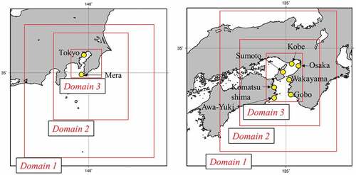
Table 6. Computational conditions for storm surge.

STOC-ML
Tokyo Bay
Grid size	D1: 2430 m, D2: 810 m, D3: 270 m
Number of grids	D1: 200 × 200, D2: 360 × 360, D3: 360 × 360
Time step	1.0 s
Osaka Bay
Grid size	D1: 2430 m, D2: 810 m, D3: 270 m
Number of grids	D1: 100 × 120, D2: 210 × 240, D3: 390 × 525
Time step	1.0 s

3. Result

In this section, we summarize the results of the typhoon forecasts for 168 cases. The accuracy of the forecasted typhoon intensity was evaluated using VRO(t) and VRC(t). Here, VR refers to variance reduction. The VR was introduced by Yamamoto et al. (2016), and they applied the VRO and VRC for several observation stations. However, in this study, these indices are used to evaluate the maximum wind speed and minimum central pressure of the typhoon by providing the VRO and VRC in the following form:

(8) $VRO\left(t\right)=1-\frac{{({\hat{y}}_t-y_t)}^2}{{y_t}^2},$(8)

(9) $VRC\left(t\right)=1-\frac{{({\hat{y}}_t-y_t)}^2}{{\widehat{y_t}}^2},$(9)

where $t$ is the hourly time step, ${\hat{y}}_t$ is the maximum wind speed or minimum central pressure calculated by WRF at time-step $t$, and $y_t$ is the same but the value in the BT. VRO and VRC take a maximum value of 1 and no lower limit. VRO and VRC take smaller values when the calculated value overestimates or underestimates the observed value, respectively. It is expedient to evaluate the “standardized” errors using VRO and VRC, rather than using conventional evaluation indexes, such as root-mean-square error because this study evaluates the computational accuracy of typhoon intensity for multiple typhoons simultaneously. Additionally, mean error ($ME$) shown as Equation (10)(10) $ME=\frac{1}{T}\sum _{t=1}^T\left({\hat{y}}_t-y_t\right),$(10) is also used for typhoon intensity evaluation to provide “not-standardized” error.

(10) $ME=\frac{1}{T}\sum _{t=1}^T\left({\hat{y}}_t-y_t\right),$(10)

where $T$ is the forecast length (h).

The typhoon track error between the location of the typhoon center (latitude and longitude) calculated by WRF and that of the BT was evaluated based on the Spherical Law of Cosines. Both track and intensity were evaluated at 6-h intervals after 12 h from the start of the typhoon simulations to consider the spin-up time of WRF.

3.1. Sensitivity of WRF’s physics options in typhoon forecast

3.1.1. Typhoon track

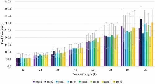
Figure 5 shows the results for the typhoon track forecast. The average forecast error was 78.4 km, 122.9 km, and 211.9 km at 24 h, 48 h, and 72 h ahead, respectively. By comparing the smallest track-error cases with the largest ones, it was observed that the track error was reduced by 9.1 km (10.9%), 11.8 km (9.1%), and 19.2 km (8.8%) at 24 h, 48 h, and 72 h ahead, respectively. For the entire time series, the reduction rate of track forecast error between the worst and best cases ranges from 6.1% (at 42 h) to 41.0% (at 96 h), with an average of 12.3%. Throughout the simulation period, from the start of forecast to 96 h ahead, relatively high accuracy of track-forecast was observed when YSU was used for PBL, especially in Case 3. The p-value for the track error throughout the entire time series was 0.9998.

Figure 5. Typhoon track forecast errors for all 168 cases. Forecast Length indicates the integration time from initialization, and the track error is evaluated for each case every 6 hours (shown every 12 hours in the figure). Gray bars indicate 95% confidence intervals for the mean of the track error.

3.1.2. Typhoon intensity

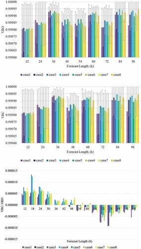
Figure 6 shows the forecast accuracy of maximum wind speed of the typhoon, and Figure 7 shows that of the minimum central pressure. The maximum wind speed is strongest at Case 2 for the first 24 h and at Case 1 during 42–66 h; hence, LIN is likely to generate the strongest typhoon in four MPs. In terms of a minimum central pressure, tendency of an underestimation was generally confirmed 48 hours ahead or later. For PBL, during 18–60 h from the beginning of the forecast simulation, the minimum central pressure of the typhoon decreases and the maximum wind speed increases using YSU than those obtained using MYJ. On the other hand, during 60–78 h, MYJ tends to generate stronger typhoons than the cases using YSU. Note that the p-value for the maximum wind speed forecast error (=1.00E-08) and the minimum central pressure forecast error (=0.00037) were very small compared with the significance level (=0.05). In other words, for typhoon intensity forecasts, the choice of physics options can cause statistically significant differences in the results obtained. Therefore, the discussion in the following subsection focuses on the case that provides the best intensity forecasting accuracy.

Figure 6. Accuracy of the maximum wind speed forecasts for all 168 cases (Top: VRO, Middle: VRC, 95% confidence intervals are shown for the mean values of VRO and VRC (gray bars). Bottom: difference between VRC and VRO. A positive value indicates that the VRO is smaller than the VRC and that the maximum wind speed is overestimated).

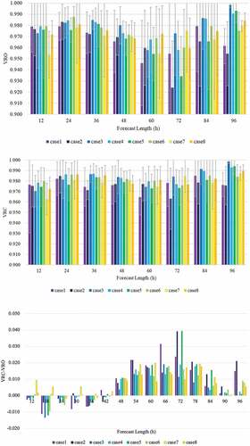
Figure 7. Same as Figure 6 but for the minimum central pressure.

3.2. Relationship between the combination of physics options that improve the accuracy of typhoon intensity forecasts and typhoon positions at initialization

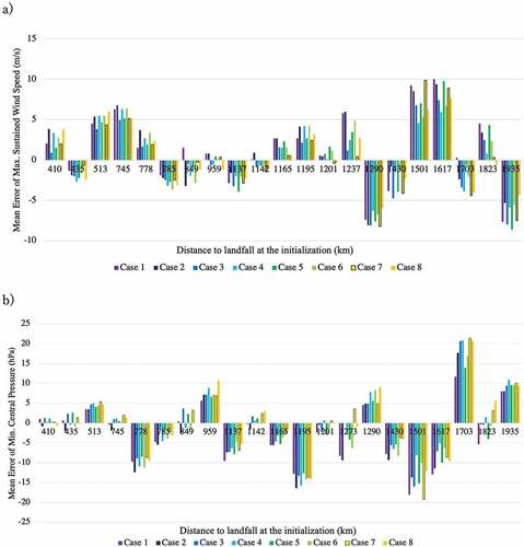
As mentioned in Section 3.1.2, the physics option with the best typhoon intensity forecast accuracy depended on the time from the start of the forecast. To explore this point further, this section discusses the relationship between the distance from the typhoon locations at initialization to landfall and the physics option that improves the accuracy of typhoon intensity forecasts. Figure 8(a-b) show the distance from the typhoon location at initialization to the landfall point and ME of the maximum wind speed and the minimum central pressure, respectively. For MP, while there are some slight differences in typhoon intensity due to differences in MP selection, they do not appear to have a significant impact on intensity forecasts compared with the impact of PBL selection. For PBL, when the typhoon location at the beginning of the forecast was not far from the landfall point (here, approximately within 1200 km), YSU provides smaller ME of the maximum sustained wind speed than MYJ. On the other hand, if the typhoon center at initialization is far from the landfall point (here, approximately more than 1200 km), the tendency changes, i.e. MYJ provides smaller ME of the maximum sustained wind speed than YSU. For the minimum central pressure, the similar tendency is seen even though some “exceptions” exist. This result suggests that PBL that achieves the highest accuracy of typhoon intensity can be dependent on the distance from typhoon location at the initialization time to the landfall point.

Figure 8. (a) Relationships between the distance to landfall point from the typhoon center locations at initialization and the Mean Error (ME) for the maximum sustained wind speed. (b) same as (a) but for the minimum central pressure.

While the abovementioned trends were confirmed, it was found that it is difficult to completely determine the best combination of physics options for each typhoon, including the “exceptions” mentioned above. Hence, the ensemble approach should be used to address the uncertainty of typhoon forecasts due to the difference in the choice of physics options in WRF. In the following section, we quantitatively evaluate the magnitude of variability in typhoon forecasts resulting from the differences in the choice of physics options. Furthermore, in Section 3.4, the performance of four cases of storm surge ensemble forecast is evaluated.

3.3. Variability in typhoon parameters at landfall due to different selections of physics options

Figure 9 shows the variability of typhoon parameters at landfall, which strongly affects storm surge forecast. The typhoon velocity varied from 25.6% to 184.5% against the observation values, the minimum central pressure varied from 0.22% to 1.6%, the maximum wind speed varied from 7.3% to 24.7%, and the approaching angle varied from 25.8° to 96.0° (the north is 0°, clockwise direction is positive; approaching angle is the amount of deviation of the direction of the typhoon from BT, calculated using values for an hour before and after, including the landfall time), the landfall points error varied in the range 25.4–103.9 km, and the landfall time error varied in the range 1–5 h, depending on the choice of physics options within one typhoon and forecast initialization time.

Figure 9. Variation in typhoon parameters of nine cases at landfall for storm surge computation. (a) landfall-time error (positive values indicate a delay relative to observations), (b) maximum wind speed, where ▲ in red is the value observed by IBTrACS. (c) approaching-angle error (clockwise direction is positive). (d) typhoon velocity in an hour before and after landfall. Typhoon velocity and approaching angle of observation are calculated using the same method as that used to evaluate WRF results. The distance traveled between two time points that straddle the time of landfall (example 15:00 and 16:00 for landfall at 15:30), divided by a time width of an hour was regarded as the typhoon velocity, and (e) is for the minimum central pressure, (f) is for the landfall-position error.

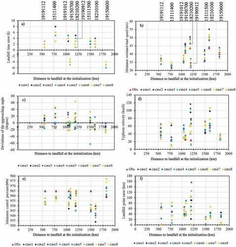
From the perspective of storm surge forecast, it should be noted that among typhoon parameters, the observed values of typhoon velocity, maximum wind speed, and approaching angle at landfall are within the range of variability of all eight WRF cases considered in this study. Furthermore, typhoon tracks and landfall points simulated by WRF are often distributed both left and right, rather than being biased to one side, relative to that of BT. From these two perspectives, the ensemble forecast using the eight combinations of physics options selected in this study can be expected to produce reasonable storm surge forecast results, compared to storm surge reanalysis simulations with a BT-driven typhoon generated using a 2D model as an external force.

3.4. Case studies of the storm surge ensemble forecast

Among the typhoons considered in this study, storm surge forecasts that predicted significant storm surges in the target areas of Tokyo and Osaka bays were performed for four typhoon events (T1919, T1915, T1821, and T1511) using cases 1–8 as ensemble members. The storm surge forecast results were compared with the JMA observations and to the results of the case where the parametric typhoon model (2D model) was used as the external force; the 2D model reproduced the typhoon using the BT (minimum central pressure, typhoon position, and typhoon velocity). Because it could reproduce the storm surge distribution reliably, it can be considered as a criterion for evaluating the validity of storm surge forecasts using WRF typhoons as an external force. In the 2D model, the pressure distribution is given by Myers’ model (Myers 1954), and the wind speed distribution is given by the equation for balancing the pressure gradient and Coriolis and centrifugal forces by considering the typhoon velocity (for details, see Supplementary Material S2).

3.4.1. T1919

Figure 10 shows the simulation results for typhoons and storm surges. The maximum storm surges for the T1919 are underestimated in Tokyo and Mera stations in the cases 19190912, 19191012, and 19191112. Storm surges are significantly underestimated in Mera, which faces the open sea. Among the three cases, case 19190912 has a large variation in the maximum wind speed and storm surge due to the landfall location of the typhoon being more varied on the east and west sides of the BT compared to the location of the typhoon in other cases. Case 19191112 had a smaller-peak storm surge variability than that in case 19191012. This can be attributed to the fact that the landfall location is biased to the left side of the BT in all eight cases (this tendency results in a smaller magnitude of the track-induced storm surge variability). The error in the peak time of storm surge could be explained using the error in the landfall time of the typhoon.

Figure 10. Upper: Typhoon forecast results for T1919. a), d), g) are the predicted typhoon tracks (6 hourly) where black line indicates the BT, b), e), h) are for the minimum central pressure and others are for the maximum sustained wind speed. Lower: Storm surge forecast results for eight cases of typhoon forecast with different WRF physics options as an external force. “Max,” “Mean,” and “Min” are the maximum, (ensemble) mean, and minimum values of storm surge at each time. “2D model” is a parametric model with the best track parameters. “Obs.” means observation. The upper line (a, c, e) shows the time series of storm surge in Tokyo, and b), d), f) are for Mera. The first column is the case of 19190912, followed by 19191012 and 19191112.

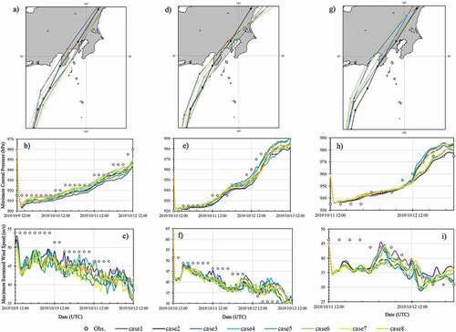
Figure 10. Continued.

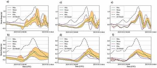
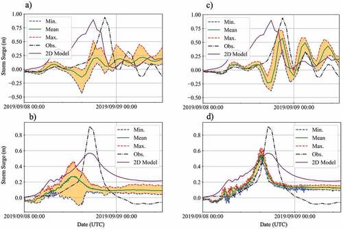
3.4.2. T1915

Figure 11 shows the simulation results for typhoons and storm surges. The maximum wind-speed average was reasonable for case 19150600 and was overestimated for case 19150700. However, storm surge was underestimated in both the case 19150600 and case 19150700. Similar to T1919, there is a tendency to underestimate the storm surge in Mera. For Tokyo, the most significant reason for the underestimation of storm surge is the misalignment of the typhoon track, where the track of the typhoon was east of the BT in all cases, and the entire Tokyo Bay was affected by the blowback wind of the typhoon, specifically in case 19150600. Notably, for T1915, the occurrence of the storm surge peak was earlier in the 2D model case than in the observation although typhoon parameters were given from the BT. The typhoon size of T1915 was very compact and did not fit well into the empirical formula for typhoon size despite its intensity. This resulted in an overestimation of typhoon size in the 2D model and an earlier landfall time, which caused an earlier storm surge onset time.

Figure 11. Same as Figure 10, but for T1915. For typhoon, the first column a)–c) are for the case 19150600, while the second column d)–f) are for case 19150700. As for storm surge, a) and b) are for case 19150600 while c), d) are for case 19150700.

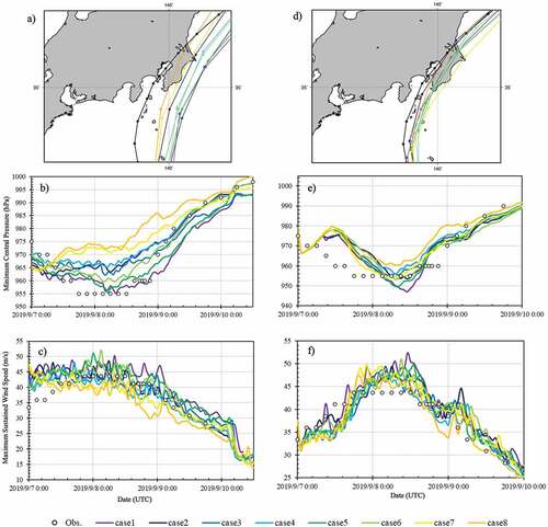
Figure 11. Continued.

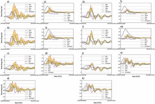
3.4.3. T1821

Figure 12 shows the simulation results for typhoons and storm surges. For cases 18210100 and 18210200, the magnitude of the variability of typhoon velocity and approaching angle are similar (Figure 9); however, the variability of storm surge for case 18210200 is considerably smaller compared to that for case 18210100. This can be attributed to two factors: the track of case 18210100 was biased to the left and right across the BT, whereas the track of case 18210200 was biased to the left of the BT in all cases, and the variation in the maximum wind speed of case 18210200 was smaller. Additionally, most storm surges were considerably underestimated in Awa-Yuki and Gobo, which are the observation points closest to the open sea among all the stations.

Figure 12. Same as Figure 10, but for T1821. For typhoon, a) – c) are for case 18210100 and d) – f) are for case 18210200. As for storm surge, a) Kobe, b) Osaka, c) Sumoto, d) Wakayama, e) Awa-yuki, f) Gobo, and g) Komatsushima. The letters on the figures are shown where a) – g) are for case 18210100, h) – n) are for 18210200.

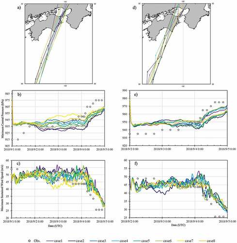
Figure 12. (Continued).

3.4.4. T1511

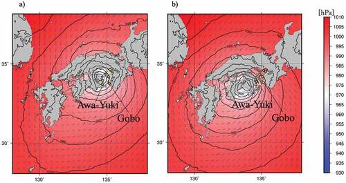
Figure 13 shows the simulation results for typhoons and storm surges. Similar to all other cases, the maximum storm surges were considerably underestimated at the stations close to the open sea, particularly in Awa-Yuki and Gobo. The maximum storm surge of case 15111400 is larger and more reasonable than that of case 15111500, which was underestimated in all cases. The landfall-location error of case 15111500 is, on an average, 10 km smaller than that of case 15111400. However, the wind direction of case 15111500 before and after the landfall was different from that of case 15111400 owing to the west-biased track of case 15111500 in all eight cases. Moreover, the atmospheric pressure around the observation point was approximately 10 hPa higher than that of case 15111400, which weakened the suction effect due to low pressure (Figure 14).

Figure 13. Same as Figure 12, but for T1511. For typhoon, a) – c) is for case 15111400 and d) – f) is for case 15111500. For storm surge, a) – g) is for case 15111400, h) – n) is for 15111500.

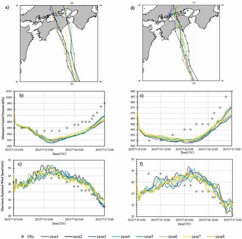
Figure 13. (Continued).

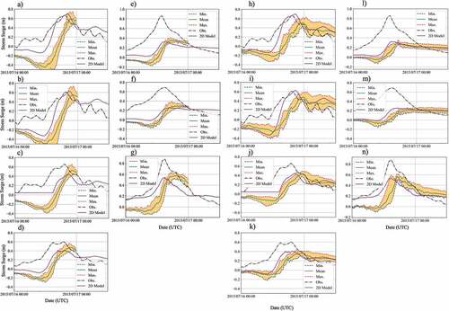
Figure 14. Pressure field (contours) and wind field (arrows) for T1511 at (a) 15111400 and (b) 15111500. Both are from Case 1. The yellow markers indicate the storm surge observation points.

3.4.5. Verification of the performance of storm surge ensemble forecasts including the four cases mentioned above

Table 7 summarizes the results of storm surge forecast and the magnitude of its variability when the ensemble mean is the average of the calculated storm surges by the eight cases using the different physics options considered in this study.

Table 7. Maximum storm surge values and magnitude of maximum storm surge variability for the eight different combinations of physics options. “Uncertainty” evaluates the magnitude of the variability of the maximum storm surge forecast simulation. It is obtained by normalizing the difference between the maximum and minimum of the maximum storm surge by using the observed values.

Typhoon	Case	Location	Max. storm surge (cal.) (m)	Max. storm surge (obs.) (m)	Uncertainty: (max-min)/obs. (cal)
T1919	19190912	Tokyo	0.501	1.380	0.828
		Mera	0.217	0.930	0.587
	19191012	Tokyo	0.588	1.380	0.646
		Mera	0.305	0.930	0.380
	19191112	Tokyo	0.830	1.380	0.560
		Mera	0.285	0.930	0.292
T1915	19150600	Tokyo	0.246	0.940	0.531
		Mera	0.260	0.910	0.333
	19150700	Tokyo	0.690	0.940	0.694
		Mera	0.523	0.910	0.212
T1821	18210100	Kobe	1.710	1.320	2.511
		Osaka	1.887	1.610	2.240
		Sumoto	1.048	0.780	2.027
		Wakayama	0.708	1.070	1.299
		Gobo	0.439	1.440	0.581
		Komatsushima	0.671	0.970	1.048
		Awa-Yuki	0.480	1.030	0.679
	18210200	Kobe	1.648	1.320	1.109
		Osaka	2.152	1.610	0.845
		Sumoto	1.088	0.780	0.909
		Wakayama	0.764	1.070	0.585
		Gobo	0.336	1.440	0.276
		Komatsushima	0.732	0.970	0.762
		Awa-Yuki	0.455	1.030	0.359
T1511	15111400	Kobe	0.575	0.660	0.700
		Osaka	0.545	0.610	0.807
		Sumoto	0.525	0.660	0.436
		Wakayama	0.477	0.610	0.415
		Gobo	0.291	0.690	0.286
		Komatsushima	0.571	0.880	0.356
		Awa-Yuki	0.343	0.860	0.258
	15111500	Kobe	0.630	0.660	0.609
		Osaka	0.482	0.610	0.651
		Sumoto	0.398	0.660	0.432
		Wakayama	0.345	0.610	0.387
		Gobo	0.259	0.690	0.314
		Komatsushima	0.642	0.880	0.794
		Awa-Yuki	0.336	0.860	0.290

Based on the time series of the simulated storm surge results presented in Section 3.4, the peak-surge values of the 2D model are almost equivalent to the ensemble means. This suggests that the storm surge forecast using WRF typhoons as an external force was averagely successful under the uncertainty in typhoon forecasts caused by differences in the selection of WRF physics options. Figure 15 shows the storm surge forecast accuracy (each case and ensemble average) obtained in this study. VRT is given by

Figure 15. The accuracy of maximum storm surge forecast conducted in this study. Plots are given every hour. (a, b) VRO-VRC, (c, d) VRT-VRC, (e, f) VRT-VRO. The second column (b, d, f) shows an enlarged view of the first column (a, c, e). “Ens. Mean” is the ensemble mean of the storm surge ensemble forecast results. VRT represents the error from the beginning of the forecast to the time when the maximum storm surge occurs; the smaller the error, the closer VRT is to 1.

(11) $VRT=1-\frac{{\left(\mathrm{\Delta }{t}_{cal}-\mathrm{\Delta }{t}_{obs}\right)}^2}{\mathrm{\Delta }{t_{obs}}^2},$(11)

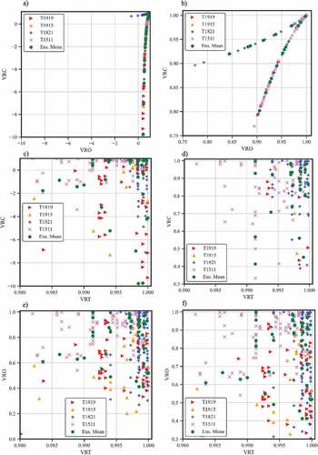
where $\mathrm{\Delta }{t}_{cal}$ is the time from the beginning of the forecast to the occurrence of the maximum storm surge in the STOC simulation and $\mathrm{\Delta }{t}_{obs}$ is the time from the beginning of the forecast to the time when the maximum storm surge was observed. VRO and VRC are derived for the maximum storm surge, and the equations are the same as Equations (8)(8) $VRO\left(t\right)=1-\frac{{({\hat{y}}_t-y_t)}^2}{{y_t}^2},$(8) and (9(9) $VRC\left(t\right)=1-\frac{{({\hat{y}}_t-y_t)}^2}{{\widehat{y_t}}^2},$(9) ).

Furthermore, there is a general trend of underestimation of the maximum storm surge except for T1821. This is due to the underestimation of the storm surge in Tokyo and other observation stations close to the open sea.

4. Discussion

We conducted sensitivity analyses of the typhoon track and intensity forecast results of the physics options of the WRF. For the track forecasts, the choice of the two PBLs (YSU and MYJ) affected the typhoon tracks rather than the choice of MPs. Particularly, the use of YSU improved the forecast accuracy of the track. Generally, YSU reproduces a more realistic boundary-layer structure (1–2 km in PBL height, approximately 4 km with MYJ, that is unrealistically thick) compared to that of MYJ (Srinivas et al. 2013). This trend was also confirmed in this study (for details, see Supplementary material S3). Thus, this may have resulted in more accurate forecasts of typhoon tracks. On the other hand, the p-value against the averaged track error for the entire time series was close to 1 so that it can be said that no statistical differences exist. In other words, all combinations considered in this study have equivalent performances in typhoon track forecasts.

For intensity forecasts, the stronger typhoons were obtained using LIN and THOMP during first 12–24 h of the forecast in terms of the maximum wind speed. According to Ming et al. (2012), the diabatic heating was larger in THOMP and LIN than that in WSM6, indicating that the typhoon intensity development was more pronounced. Moreover, they stated that, because of the manner THOMP handles the size of the snow it employs, it produces considerable snow. The snow caused low amount of cloud ice in the upper sky, which was confirmed in this study (for detail, see Supplementary material S3). These cloud microphysical processes related to snow generation and growth (generates snow, depositional growth) accelerate diabatic heating and make the typhoons stronger, specifically in the first 24 h of the forecast. Furthermore, for the minimum central pressure, the use of LIN strengthened the typhoons specifically after 48 h. Ming et al. (2012) mentioned that the more diabatic heating occurs in supersaturated conditions when large amounts of water vapor condense into cloud water or deposit as cloud ice. These trends may have strengthened the typhoon intensity with LIN throughout the entire time series. For WSM5 and WSM6, Chan and Chan (2016) demonstrated that the effect of the presence of graupel on typhoon intensity is not significant, and the results of this study concur. Although it is necessary to examine these physical behaviors in more detail, we omit them because they are slightly beyond the scope of this study.

Paying attention to the distance from typhoon positions at the initialization time to the landfall points, the use of YSU for PBL improved the accuracy of typhoon intensity forecast if the distance is within approximately 1200 km as mentioned in Section 3.2. Conversely, if the distance exceeds 1200 km, MYJ tended to provide a better accuracy of typhoon intensity forecasts than YSU. This is because MYJ produced weaker typhoons than YSU in cases 19150600, 16092000, and 16071400 (the distance exceeds 1200 km in these cases) when the maximum wind speed was overestimated, while YSU tended to produce weaker typhoons than MYJ in the other typhoon cases, as can be seen from Figure 8a. Interestingly, these three typhoons (T1607, T1609, and T1915) have similar characteristics (combinations of typhoon parameters shown in Figure 1, such as typhoon size, typhoon intensity, and typhoon velocity) compared to the other six typhoons covered by this study.

Notably, when sea-surface temperatures decrease owing to ocean mixing associated with typhoon passage, over-strengthening in the latter half of the typhoon intensity forecast is suppressed, resulting in a high forecast accuracy (Ito et al. 2015). In this study, the typhoon intensity is tended to overestimate in the latter half of the forecast owing to the constant sea-surface temperatures included in the initial conditions. Therefore, the effect of ocean mixing on WRF should be introduced to improve the intensity forecast accuracy.

For the storm surge forecast results, the maximum storm surges in T1821 and T1511 showed a large underestimation tendency in Gobo and Awa-Yuki. In T1919 and T1915, the maximum storm surge was significantly underestimated in Mera, which faces the open sea, similar to Gobo and Awa-Yuki. A possible cause of the underestimation of storm surges in these locations is not considering sea-level-rise effect due to wave setup in STOC-ML model. During the passage of typhoons or low-pressure systems, the tide level at the open-ocean points such as Mera and Gobo rose significantly due to wave setup, compared to that in the inner bay areas (Japan Meteorological Agency 2021). Moreover, according to Japan Meteorological Agency (2021), the wave setup was more pronounced in the open-sea area during T1915 (up to 60 cm rise by wave setup) and T1919.

In terms of typhoon forecast accuracy as an external force of storm surge, even a 10 km shift in the landfall location of a typhoon can significantly change the predicted results of storm surge (Kohno et al. 2018). It may be considered that the effect of wind setup is not well incorporated in some underestimated cases in the results. Employing data assimilation is an effective way to improve typhoon track forecasting accuracy (Shen et al. 2021), which is not considered in this study.

From the perspective of utilizing forecasts for evacuation support, it is preferable to obtain reasonable storm surge forecast results in the process as early as possible. However, it is difficult to eliminate relatively long-term forecast errors especially in track forecast because the errors generally increase as the forecast time increases, like the results of this study. Thus, probabilistic forecast is required in long-term forecast. Xie et al. (2021) developed a method for generating a typhoon ensemble by applying perturbations to parameters such as typhoon velocity and approaching angle, and for searching the storm surge database for fast and accurate forecasts utilizing the “probability circle” concept. This method of utilizing such databases is effective in minimizing computational time and cost during real-time typhoon and ensemble storm surge forecasts.

Future challenges include the use of probabilistic forecast methods such as the ensemble forecast performed in this study and the use of databases to realize a storm surge forecast system with high accuracy, including long-term forecasts, at a relatively low cost.

For instance, the ensemble forecast method can be applied to other computational conditions apart from the physics options (grid resolutions, initial and boundary conditions, and domain size). However, if ensemble simulations are performed for all computational conditions to account for variations in typhoon forecasts, numerous cases will be required, which is undesirable from the perspective of real-time forecast. Therefore, it is necessary to devise a method for estimating the magnitude of forecast uncertainty associated with the selection of WRF computational conditions by utilizing database (in this study, it is composed of 168 cases of WRF simulations) to calculate confidence intervals of forecast errors as shown in Figures 5–7 and to efficiently perform probabilistic typhoon and storm surge forecast without calculating all ensemble members in real-time.

5. Conclusion

WRF is extremely useful as a method for forecasting typhoons as an external force for storm surge forecast. However, several combinations of physics options exist in WRF, and the typhoon forecast results vary based on their selection. Moreover, the combination of the physics options with the highest typhoon forecast accuracy is different for each typhoon. Therefore, it is difficult to determine the physics option that should be used in typhoon forecast.

In this study, we reviewed the previous studies on sensitivity analysis of physics options for typhoon forecasting using WRF and summarized the physics options that have been used frequently. Specifically, we focused on cloud microphysics (MP), and planetary boundary layer (PBL), that are known to have a significant effect on typhoon forecast results.

Considering these results, sensitivity analyses were conducted using the physics options that are widely used or expected to have higher typhoon forecast accuracy in the Western Pacific region: the MPs are LIN, WSM5, WSM6, and THOMP and PBLs are YSU and MYJ. In the sensitivity analyses, we quantitatively evaluated the variability of typhoon and storm surge forecasts due to differences in the selection of the physics options of WRF for several typhoons that caused landfall in Japan.

The sensitivity analyses confirmed that the use of YSU for PBL increases the accuracy of typhoon track forecast, while all combinations of physics options considered in this study provided a comparable accuracy of typhoon track forecasts. In the results of typhoon intensity forecasts, the trend was clearly changed by altering the MP and PBL, as shown in Section 3.1.2. Additionally, the combination of physics options that improved the accuracy of the intensity forecasts also tends to depend on the distance between the typhoon location at initialization and the landfall point, as shown in Section 3.2. Note that a few kilometers of deviations of the typhoon track affect the storm surge forecast so that it is necessary to address the variability in typhoon forecast due to the choice of physics options, while no “best combination” of physics options exists. Therefore, after quantitatively evaluating the variability of typhoon parameters at landfall in Section 3.3, storm surge ensemble forecasts were performed to investigate the uncertainty propagated to the storm surge forecasts from the typhoon forecasts.

Notably, the uncertainty associated with storm surge forecast varies depending on the external forces and topography of the target area. Therefore, it is necessary to investigate the mode of uncertainty propagation from typhoon forecasts to storm surge forecasts for other typhoons and regions. In this context, the authors hope that the information on the uncertainty in storm surge forecasts due to the variability of typhoon forecasts caused by different settings of computational conditions in weather forecasting models presented in this study will be effectively used in related research and/or an evacuation assistance in the future.

Acknowledgments

This research was conducted as part of the Earth Simulator application project “Superimposed Disasters of Heavy Rainfall, Storm Surge and Tsunami” (Research director: T. Arikawa) of the Japan Agency for Marine-Earth Science and Technology (JAMSTEC) and utilized the computing resources of the Earth Simulator. The work was also supported by “Collaborative Research Project on Computer Science with High-Performance Computing in Nagoya University”.

Disclosure statement

No potential conflict of interest was reported by the author(s).

Supplementary material

Supplemental data for this article can be accessed online at https://doi.org/10.1080/21664250.2022.2124040

References

- Alam, M.M. 2020. “Sensitivity Study of Planetary Boundary Layer Parameterization Schemes for the Simulation of Tropical Cyclone ‘FANI’ over the Bay of Bengal Using High Resolution WRF-ARW Model.” Journal of Engineering Science 11 (2): 1–18. doi:10.3329/jes.v11i2.50893.
- Bopape, M.-J. M., H. Cardoso, R. S. Plant, E. Phaduli, H. Chikoore, T. Ndarana, E. Rakate, and E. Rakate. 2021. “Sensitivity of Tropical Cyclone Idai Simulations to Cumulus Parametrization Schemes.” Atmosphere 12 (8): 932. doi:10.3390/atmos12080932.
- Chan, K. T. F., and J. C. L. Chan. 2016. “Sensitivity of the Simulation of Tropical Cyclone Size to Microphysics Schemes.” Advances in Atmospheric Sciences 33 (9): 1024–1035. doi:10.1007/s00376-016-5183-2.
- Chandrasekar, R., and C. Balaji. 2012. “Sensitivity of Tropical Cyclone Jal Simulations to Physics Parameterizations.” Journal of Earth System Science 121 (4): 923–946. doi:10.1007/s12040-012-0212-8.
- Chen, S., Yk. Qian, and S. Peng. 2015. “Effects of Various Combinations of Boundary Layer Schemes and Microphysics Schemes on the Track Forecasts of Tropical Cyclones Over the South China Sea.” Nat Hazards 78: 61–74. doi:10.1007/s11069-015-1697-7.
- Chen, S.-H., and W.-Y. Sun. 2002. “A One-dimensional Time Dependent Cloud Model.” Journal of the Meteorological Society of Japan 80 (1): 99–118. doi:10.2151/jmsj.80.99.
- Choudhury, D., and S. Das. 2017. “The Sensitivity to the Microphysical Schemes on the Skill of Forecasting the Track and Intensity of Tropical Cyclones Using WRF-ARW Model.” Journal of Earth System Science 126 (4): 57. doi:10.1007/s12040-017-0830-2.
- Davis, C., W. Wang, S.-S. Chen, Y. Chen, K. Corbosiero, M. DeMaria, J. Dudhia, et al. 2008. “Prediction of Landfalling Hurricanes with the Advanced Hurricane WRF Model.” Monthly Weather Review 136 (6): 1990–2005. doi:10.1175/2007MWR2085.1.
- Di, Z., W. Gong, Y. Gan, C. Shen, and Q. Duan. 2019. “Combinatorial Optimization for WRF Physical Parameterization Schemes: A Case Study of Three-day Typhoon Simulations over the Northwest Pacific Ocean.” Atmosphere 10 (5): 233. doi:10.3390/atmos10050233.
- Douluri, D. L., and K. Annapurnaiah. 2016. “Impact of Microphysics Schemes in the Simulation of Cyclone Hudhud Using WRF-ARW Model.” International Journal of Oceans and Oceanography 10 (1): 49–59.
- Douluri, D. L., P. L. N. Murty, P. K. Bhaskaran, B. Sahoo, T. S. Kumar, S. S. C. Shenoi, and A. S. Srikanth. 2017. “Performance of WRF-ARW Winds on Computed Storm Surge Using Hydrodynamic Model for Phailin and Hudhud Cyclones.” Ocean Engineering 131: 135–148. doi:10.1016/j.oceaneng.2017.01.005.
- Fovell, R. G., and H. Su. 2007. “Impact of Cloud Microphysics on Hurricane Track Forecasts.” Geophysical Research Letters 34 (24): 24. doi:10.1029/2007GL031723.
- “GEBCO 30 arc-seconds Grid” https://www.gebco.net/data_and_products/gridded_bathymetry_data/gebco_30_second_grid/ ( final reference: 26 March 2021
- Hill, K. A., and G. M. Lackmann. 2009. “Analysis of Idealized Tropical Cyclone Simulations Using the Weather Research and Forecasting Model: Sensitivity to Turbulence Parameterization and Grid Spacing.” Monthly Weather Review 137 (2): 745–765. doi:10.1175/2008MWR2220.1.
- Honda, K., R. Naito, and T. Asai. 2016. “Damage to Port Areas along Seto Inland Sea Due to Storm Surge and Waves of Typhoon 1511.” Technical Note of NILIM, 893: 1–40.
- Hong, S.–Y., D. Jimy, and S.–H. Chen. 2004. “A Revised Approach to Ice Microphysical Processes for the Bulk Parameterization of Clouds and Precipitation.” Monthly Weather Review 132 (132): 103–120. doi:10.1175/1520-0493(2004)132<0103:ARATIM><0103:ARATIM>2.0.CO;2.
- Hong, S.Y., and J. O. J. Lim. 2006. “The WRF Single-moment 6-class Microphysics Scheme (WSM6).” Journal of Korean Meteorological Society 42: 129–151.
- Hong, S.–Y., N. Yign, and D. Jimy. 2006. “A New Vertical Diffusion Package with an Explicit Treatment of Entrainment Processes.” Monthly Weather Review 134 (134): 2318–2341. doi:10.1175/MWR3199.1.
- Islam, T., P.K. Srivastava, M.A. R-Ramirez, Q. Dai, M. Gupta, and SK. Singh. 2015. “Tracking a Tropical Cyclone through WRF–ARW Simulation and Sensitivity of Model Physics.” Natural Hazards 76 (3): 1473–1495. doi:10.1007/s11069-014-1494-8.
- Ito, K., T. Kuroda, K. Saito, and A. Wada. 2015. “Forecasting a Large Number of Tropical Cyclone Intensities around Japan Using a High-resolution Atmosphere–ocean Coupled Model.” Weather and Forecasting 30 (3): 793–808. doi:10.1175/WAF-D-14-00034.1.
- Jang, D., W. Joo, C.-H. Jeong, W. Kim, S. W. Park, and Y. Song. 2020. “The Downscaling Study for Typhoon-induced Coastal Inundation.” Water 12 (4): 1103. doi:10.3390/w12041103.
- Janjic, Z. I. 1994. “The Step-mountain Eta Coordinate Model: Further Developments of the Convection, Viscous Sublayer and Turbulence Closure Schemes.” Monthly Weather Review 122 (122): 927–945. doi:10.1175/1520-0493(1994)122<0927:TSMECM>2.0.CO;2.
- Japan Meteorological Agency, 2021. “Storm Surge Models and Their Use - Forecasting Work in Storm Surge Cases.” https://www.jma.go.jp/jma/kishou/know/expert/pdf/r2_text/r2_takashio.pdf ( Final Access, 5 January 2022
- Kanase, R. D., Salvekar, and P S. Salvekar. 2015. “Impact of Physical Parameterization Schemes on Track and Intensity of Severe Cyclonic Storms in Bay of Bengal.” Meteorology and Atmospheric Physics 127 (5): 537–559. doi:10.1007/s00703-015-0381-5.
- Kim, S. Y., T. Matsuura, Y. Matsumi, K. Tamai, T Yasuda, T. H. Tom, and H. Mase. 2013. Effects of WRF Parameterization on Meteorological Predictions in the mid-latitude Region – Planetary Boundary Layer Scheme and Cloud Microphysics. Journal of Japan Society of Civil Engineers Ser B2 (Coastal Engineering). in Japanese 69 2: I_516–I_520. 10.2208/kaigan.69.I_516.
- Kloetzke, T., M. S. Mason, and R. J. Krupar, 2016. “Sensitivity of WRF-ARW Simulations to the Choice of Physics Parameterization Schemes When Reconstructing Tropical Cyclone Ita (2014)” 18th Australasian Wind Engineering Society Workshop McLaren Vale, South Australia, 6-8 July 2016.
- Kohno, N., S. K. Dube, M. Entel, S. H. Fakhruddin, D. Greenslade, M.-D. Leroux, J. Rhome, and N. B. Thuy. 2018. “Recent Progress in Storm Surge Forecasting.” Tropical Cyclone Research and Review 7 (2): 128–139. doi:10.6057/2018TCRR02.04.
- Li, J., Y. Hou, D. Mo, Q. Liu, and Y. Zhang. 2019. “Influence of Tropical Cyclone Intensity and Size on Storm Surge in the Northern East China Sea.” Remote Sensing 11 (24): 3033. doi:10.3390/rs11243033.
- Lin, N., K. Emanuel, M. Oppenheimer, and E. Vanmarcke. 2012. “Physically Based Assessment of Hurricane Surge Threat under Climate Change.” Nature Climate Change 2 (6): 462–467. doi:10.1038/NCLIMATE1389.
- Li, X., and Z. Pu. 2008. “Sensitivity of Numerical Simulation of Early Rapid Intensification of Hurricane Emily (2005) to Cloud Microphysical and Planetary Boundary Layer Parameterizations.” Monthly Weather Review 136 (12): 4819–4838. doi:10.1175/2008MWR2366.1.
- Li, X., and Z. Pu. 2009. “Sensitivity of Numerical Simulations of the Early Rapid Intensification of Hurricane Emily to Cumulus Parameterization Schemes in Different Model Horizontal Resolutions.” Journal of the Meteorological Society of Japan 87 (3): 403–421. doi:10.2151/jmsj.87.403.
- Maldonado, T., J.A. Amador, R.R. Rivera, H.G. Hidalgo, and E.J. Alfaro. 2020. “Examination of WRF-ARW Experiments Using Different Planetary Boundary Layer Parameterizations to Study the Rapid Intensification and Trajectory of Hurricane Otto (2016).” Atmosphere 11 (12): 1317. doi:10.3390/atmos11121317.
- Maw, K.-W., J. Min. 2017. “Impacts of Microphysics Schemes and Topography on the Prediction of the Heavy Rainfall in Western Myanmar Associated with Tropical Cyclone ROANU (2016).” Advances in Meteorology 2017: 22 doi:10.1155/2017/3252503.
- Mesinger, F.1993.“Forecasting Upper Tropospheric Turbulence within the Framework of the Mellor-Yamada 2.5 Closure.”Research Activities in Atmospheric and Oceanic Modelling WMO 18: 4.28–4.29. Geneva, CAS/JSC WGNE Rep.
- Ming, J., S. Shu, Y. Wang, J. Tang, and B. Chen. 2012. “Modeling Rapid Intensification of Typhoon Saomai (2006) with the Weather Research and Forecasting Model and Sensitivity to Cloud Microphysical Parameterizations.” Journal of the Meteorological Society of Japan 90 (5): 771–789. doi:10.2151/jmsj.2012-513.
- Musinguzi, A., M. K. Akbar, J. G. Fleming, and S. K. Hargrove. 2019. “Understanding Hurricane Storm Surge Generation and Propagation Using a Forecasting Model, Forecast Advisories and Best Track in a Wind Model, and Observed Data-case Study Hurricane Rita.” Journal of Marine Science and Engineering 7 (3): 77. doi:10.3390/jmse7030077.
- Myers, V.A. 1954. “Characteristics of United States Hurricanes Pertinent to Levee Design for Lake Okechobee, Florida.” In Hydrometeorologic Reports. Vol. 32. Weather Bureau: U.S. Department of Commerce. 1–106.
- Nasrollahi, N., A. AghaKouchak, J. Li, X. Gao, K. Hsu, and S. Sorooshian. 2012. “Assessing the Impacts of Different WRF Precipitation Physics in Hurricane Simulations.” Weather and Forecasting 27 (4): 1003–1016. doi:10.1175/WAF-D-10-05000.1.
- National Centers for Environmental Prediction/National Weather Service/NOAA/U.S. Department of Commerce. 2015, updated daily. NCEP GDAS/FNL 0.25 Degree Global Tropospheric Analyses and Forecast Grids. Research Data Archive at the National Center for Atmospheric Research, Computational and Information Systems Laboratory. Accessed 1 September, 2022. doi:10.5065/D65Q4T4Z
- National Centers for Environmental Prediction/National Weather Service/NOAA/U.S. Department of Commerce. 2015, updated daily. NCEP GFS 0.25 Degree Global Forecast Grids Historical Archive. Research Data Archive at the National Center for Atmospheric Research, Computational and Information Systems Laboratory. Accessed 1 September, 2022. doi:10.5065/D65D8PWK
- Nolan, D.S., D.P. Stern, and J.A. Zhang. 2009. “Evaluation of Planetary Boundary Layer Parameterizations in Tropical Cyclones by Comparison of in Situ Observations and High-Resolution Simulations of Hurricane Isabel (2003). Part II: Inner-Core Boundary Layer and Eyewall Structure.” Monthly Weather Review 137 (11): 3675–3698. doi:10.1175/2009MWR2786.1.
- Osuri, K. K., U. C. Mohanty, A. Routray, M. A. Kulkarni, and M. Mohapatra. 2012. “Customization of WRF-ARW Model with Physical Parameterization Schemes for the Simulation of Tropical Cyclones over North Indian Ocean.” Natural Hazards 63 (3): 1337–1359. doi:10.1007/s11069-011-9862-0.
- Park, J., D.-H. Cha, M.K. Lee, J. Moon, S.-J Hahm, K. Noh, C.L.C. Johnny, and B. Michael. 2020. “Impact of Cloud Microphysics Schemes on Tropical Cyclone Forecast over the Western North Pacific.” Journal of Geophysical Research: Atmospheres 125: e2019JD032288. doi:10.1029/2019JD032288.
- Powers, J. G., J. B. Klemp, W. C. Skamarock, C. A. Davis, J. Dudhia, D. O. Gill, and M. G. Duda. 2017. “The Weather Research and Forecasting Model: Overview, System Efforts, and Future Directions.” Bulletin of the American Meteorological Society 98 (8): 1717–1737. doi:10.1175/BAMS-D-15-00308.1.
- Rajeswari, J. R., C. V. Srinvas, P. Reshimi Mohan, and B. Venkatraman. 2020. “Impact of Boundary Layer Physics on Tropical Cyclone Simulations in the Bay of Bengal Using the WRF Model.” Pure and Applied Geophysics 177 (2020): 5523–5550. doi:10.1007/s00024-020-02572-3.
- Reddy, M. V., S B S. Prasad, U V M. Krishna, and K. K. Reddy. 2014. “Effect of Cumulus and Microphysical Parameterizations on the JAL Cyclone Prediction.” Indian Journal of Radio & Space Physics 43: 103–123.
- Saikumar, P. J., and T. Ramashri. 2017. “Impact of Physics Parameterization Schemes in the Simulation of Laila Cyclone Using the Advanced Mesoscale Weather Research and Forecasting Model.” International Journal of Applied Engineering Research 12 (22): 12645–12651.
- Saikumar, P. J., and T. Ramashri. 2018. “Impact of Microphysics Parameterization Schemes in Simulation of Vardah Cyclone Using the Advanced Mesoscale Weather Research and Forecasting Model.” International Journal of Engineering & Technology 7 (3.29): 272–274. doi:10.14419/ijet.v7i3.29.18809.
- Shen, F., A. Shu, H. Li, D. Xu, and J. Min. 2021. “Assimilation of Himawari-8 Imager Radiance Data with the WRF-3DVAR System for the Prediction of Typhoon Soudelor.” Natural Hazards and Earth System Sciences 21 (5): 1569–1582. doi:10.5194/nhess-21-1569-2021.
- Shirai, T., K. Fujiwara, M. Watanabe, and T. Arikawa. 2020. “A Study of Computation Time and Accuracy of the Prediction of Storm Surge and Waves Using Global WRF Model.” Journal of Japan Society of Civil Engineers Ser B2 (Coastal Engineering) 76 (2): I_247–I_252. doi:10.2208/kaigan.76.2_I_247. Japanese.
- Skamarock, W. C., J. B. Klemp, J. Dudhia, D. O. Gill, D. Barker, M. G. Duda, X.-y. Huang, W. Wang, and J. G. Powers. 2008. “A Description of the Advanced Research WRF Version 3.” NCAR Technical Notes 113. NCAR/TN-4751STR. doi:10.5065/D68S4MVH.
- Srinivas, C.V., D. B. Rao, V. Yesubabu, R. Baskaran, and B. Venkatraman. 2013. “Tropical Cyclone Predictions over the Bay of Bengal Using the high-resolution Advanced Research Weather Research and Forecasting (ARW) Model.” Quarterly Journal of the Royal Meteorological Society 139 (676): 1810–1825. doi:10.1002/qj.2064.
- Sun, Y., Z. Zhong, and W. Lu. 2015. ””Sensitivity of Tropical Cyclone Feedback on the Intensity of the Western Pacific Subtropical High to Microphysics Schemes.” Journal of the Atmospheric Sciences.” 72 (4): 1346–1368. doi:10.1175/JAS-D-14-0051.1.
- Tang, j., J. A. Zhang, C. Kieu, and F. D. Marks. 2018. “Sensitivity of Hurricane Intensity and Structure to Two Types of Planetary Boundary Layer Parameterization Schemes in Idealized HWRF Simulations.” Tropical Cyclone Research and Review 7 (4): 201–211. doi:10.6057/2018TCRR04.01.
- Tao, WK., J.J. Shi, S.S. Chen, S. Lang, P-L Lin, S.-Y. Hong, Christa P.-Lidard, and A. Hou. 2011. “The Impact of Microphysical Schemes on Hurricane Intensity and Track.” Asia-Pacific Journal of Atmospheric Sciences 47 (1): 1–16. doi:10.1007/s13143-011-1001-z.
- Thompson, G., P. R. Field, R. M. Rasmussen, and W. D. Hall. 2008. “Explicit Forecasts of Winter Precipitation Using an Improved Bulk Microphysics Scheme. Part II: Implementation of a New Snow Parameterization.” Monthly Weather Review 136 (136): 5095–5115. doi:10.1175/2008MWR2387.1.
- Tomita, T., and T. Kakinuma. 2005. “Storm Surge and Tsunami Simulator in Oceans and Coastal Areas (STOC).”Report of the Port and Airport Research Institute 44 (2) 83–98 in Japanese
- Torres, M.J., M.R. Hashemi, S. Hayward, M. Spaulding, I. Ginis, and S. Grilli. 2019. “Role of Hurricane Wind Models in Accurate Simulation of Storm Surge and Waves.” Journal of Waterway, Port, Coastal, and Ocean Engineering 145 (1). doi:10.1061/(ASCE)WW.1943-5460.0000496.
- Tsai, Y.-L., T.-R. Wu, C.-Y Lin, S. C. Lin, E. Yen, and C. W. Lin. 2020. “Discrepancies on Storm Surge Predictions by Parametric Wind Model and Numerical Weather Prediction Model in a Semi-enclosed Bay: Case Study of Typhoon Haiyan.” Water 12 (12): 3326. doi:10.3390/w12123326.
- Valle, A. N. R., E. N. Curchitser, and C. L. Bruyere. 2020. “Impact of Tropical Cyclone Landfall Angle on Storm Surge along the Mid‐Atlantic Bight.” Journal of Geophysical Research: Atmospheres 125: e2019JD031796. doi:10.1029/2019JD031796.
- Valle, A. N. R., E. N. Curchitser, C. L. Bruyere, and K. R. Fossell. 2018. “Simulating Storm Surge Impacts with a Coupled Atmosphere-inundation Model with Varying Meteorological Forcing.” Journal of Marine Science and Engineering 6 (2): 35. doi:10.3390/jmse6020035.
- Wannawong, W., D. Wang, Y. Zhang, and C. Ekkawatpanit. 2018. “Sensitivity of Different Parameterizations on Simulation of Tropical Cyclone Durian over the South China Sea Using Weather Research and Forecasting (WRF) Model.” Preprint. doi:10.20944/preprints201804.0336.v1.
- Wu, Z., C. Jiang, B. Deng, J. Chen, and X. Liu. 2019. “Sensitivity of WRF Simulated Typhoon Track and Intensity over the South China Sea to Horizontal and Vertical Resolutions.” Acta Oceanologica Sinica 38 (7): 74–83. doi:10.1007/s13131-019-1459-z.
- Xie, Y., S. Shang, J. Chen, F. Zhang, Z. He, G. Wei, J. Wu, B. Zhu, and Y. Zeng. 2021. “Fast Storm Surge Ensemble Prediction Using Searching Optimization of a Numerical Scenario Database.” Weather and Forecasting 36 (5): 1629–1648. doi:10.1175/WAF-D-20-0205.1. Retrieved 5 March 2022.
- Yamamoto, N., S. Aoi, K. Hirata, W. Suzuki, T. Kunugi, and H. Nakamura. 2016. “Multi-index Method Using Offshore Ocean-bottom Pressure Data for Real-time Tsunami Forecast.” Earth, Planets and Space 68 (128). doi:10.1186/s40623-016-0500-7.
- Zhang, F., M. Li, A. C. Ross, S. B. Lee, and D.-L. Zhang. 2017. “Sensitivity Analysis of Hurricane Arthur (2014). Storm Surge Forecasts to WRF Physics Parameterizations and Model Configurations.” Weather and Forecasting 32 (5): 1745–1764. doi:10.1175/WAF-D-16-0218.1.