Future changes in extreme storm surge based on a maximum potential storm surge model for East Asia

ABSTRACT

We analyzed tropical cyclones (TC) based on the theory of Maximum Potential Intensity (MPI) and Maximum Potential Surge (MPS) for a long-term assessment of extreme TC intensity and storm surge heights. We investigated future changes in the MPI fields and MPS for different global warming levels based on 150-year continuous scenario projections (HighResMIP) and large ensemble climate projections (d4PDF/d2PDF). Focusing on the Western North Pacific Ocean (WNP), we analyzed future changes in the MPI and found that it reached a maximum in the latitudinal range of 30–40°N in September. We also analyzed future changes in the MPS in major bays of East Asia and along the Pacific coast of Japan. Future changes in the MPS were projected, and it was confirmed that changes in the MPS are larger in bays where large storm surge events have occurred in the past.

KEYWORDS:

• Climate change
• extreme storm surge
• maximum potential intensity
• maximum potential surge

1. Introduction

Based on climate projections that consider global warming, various impact assessments have been made for temperature, precipitation, water resources, and sea-level rise (e.g. the series of Assessment Reports by the Intergovernmental Panel on Climate Change (IPCC)). In coastal areas, sea-level rise is mainly important as a gradual change in the coastal environment, while extreme events such as tropical cyclones (TC) are expected to have a significant impact on storm surges. Global warming is expected to affect the characteristics of TCs, such as frequency, intensity, and tracks. In the Sixth Assessment Report (AR6; Sixth Assessment Report of the IPCC, 2021) and Special Report on the Ocean and Cryosphere (SROCC; Pörtner et al. 2019), the IPCC suggests that the number of TCs generated in the future will be fewer overall, but the intensities will be stronger on a global scale. In addition, the number of intense TC (categories 4–5) is expected to increase from present-day values because of climate change (e.g. Emanuel 2013; Yoshida et al. 2017; AR6, 2021). However, future TC characteristics changes are still uncertain on regional and global scales.

Many adaptation measures against global warming depend directly on TC-related natural hazard risk assessments (e.g. Mori and Takemi 2016; Mori et al. 2021a). Therefore, it is necessary to project future changes of extremes in intensity and frequency for disaster risk management, disaster countermeasure planning, and other adaptations. For example, the Summary for Policymakers (SPM) of AR6 states that “In coastal cities, the combination of more frequent extreme sea level events (due to sea level rise and storm surge) and extreme rainfall/river flow events will make flooding more probable (high confidence).” Additionally, the AR6 SPM warns that low-likelihood consequences of future warming cannot be excluded and are part of the risk assessment. Therefore, assessing extreme storm surges in a future climate is important for developing adaptation strategies in low-lying coastal areas in the mid-latitudes of the Pacific, North Atlantic, and Indian Oceans. However, the number of observed extreme storm surge events is extremely limited (e.g. Typhoon Haiyan by Tajima et al. 2014; Typhoon Jebi by Mori et al. 2019b), and therefore, it is difficult to conduct a probabilistic assessment of extreme storm surge based on historical events only.

Increasing the number of extreme events, both for statistical and dynamic modeling, is helpful for analyzing the extremes. A stochastic TC model (e.g. Nakajo et al. 2014), a kind of emulator, can increase the number of TCs via a Monte Carlo simulation. It has been widely used for strong wind engineering and storm surge assessment. However, the stochastic TC model is generally calibrated using historical data; therefore, it is not easy to implement the effects of climate change into the model. On the other hand, a climate projection based on a global climate model (GCM) forced by a greenhouse gas emission scenario (GHE), can produce long-term climatological data (i.e. virtual/synthetic) that is longer than the historical record. Many storm surge assessments have been performed using a dynamic storm surge model forced by GCM-derived sea surface pressure and wind fields (e.g. Yasuda et al., 2014). However, until the arrival of the Coupled Model Intercomparison Project 5 (CMIP5), the duration of the climate projection has generally been limited to 100 years. Extreme wind, river flood, and coastal flood events, which are important for infrastructure development and evacuation planning, are conducted for frequencies of 1 by 50 years to 1 by hundreds of years. Considering the uncertainty of the extreme value estimation, it is difficult to project the future change of extreme wind and river and coastal flood events with a climate projection of 100 years. In 2016, a large ensemble climate projection experiment spanning over 5000 years was conducted by a Japanese team using a single atmospheric GCM (AGCM) (Mizuta et al. 2017; Ishii and Mori 2020), and the experiment is now beginning to be used for impact assessments of extremes (e.g. Ishii and Mori 2020). The number of TC events that can be used for analysis has dramatically increased in both the present and future climate conditions.

Dynamic storm surge models (i.e. shallow water equation models) have generally been used to simulate storm surges for stochastic and synthetic events. The accuracy of the dynamical model-based prediction is satisfactory for simulating the storm surges of a particular historical TC (e.g. Mori et al. 2014; Mikami et al. 2016; Mori et al. 2019b; Toyoda, Yoshino, and Kobayashi 2022a). In addition, several studies on assessing the impact of climate change on the storm surges for specific bays have been conducted based on historical events, so-called pseudo global warming experiments (PGW experiments). The PGW experiment quantitatively projects how a given past typhoon and storm surge would change in a future climate (e.g. Takayabu et al. 2015; Ninomiya et al. 2017; Nakamura et al. 2020; Toyoda et al. 2022b). However, it projects a limited figure under restricted conditions. An alternative approach is directly driving the dynamic storm surge model by the GCM results (e.g. Kim et al. 2017; Shimura et al. 2022). This approach is straightforward but can only be used for calculations up to 100 years at most. The simulations for periods longer than 1,000 years are virtually impossible.

Therefore, it is difficult to use a dynamic model to simulate storm surge for a long-term assessment if the number of TC events or period length is increased dramatically using stochastic or climatological models. The computational costs of this approach are a major challenge for very long climate simulations of 1000 years or longer (e.g. Kumagai, Mori, and Nakajo 2016; Wahl, Mudersbach, and C 2015; Igarashi et al., 2021; Gönnert et al. 2015). In order to reduce computational costs, a simplified model based on climatological information keeping physical essence and accuracy is needed to assess long-term climate change impacts on extreme storm surges (Mori et al. 2019a). The challenge is developing a projection method that balances computational accuracy, modeling, and cost. Since storm surge is a localized phenomenon (with a scale of tens to a few hundred kilometers), each bay has different storm surge characteristics caused by different geometrical features. Therefore, conducting a global or regional scale assessment is necessary to identify regions that are most at risk due to climate change. On the other hand, if we assume that a typhoon of maximum intensity passes over a particular bay at a path and speed that maximizes wind-induced surge, we can estimate the maximum class of storm surge. In parallel with dynamic storm surge projection based on climate projections, it is also necessary to make projections of the maximum class storm surges based on the above-mentioned progress in research on climate change projections and impact assessments.

Mori et al. (2021b) developed a framework to seamlessly project the climatic maximum potential surge (MPS; sea surface anomaly height excluding astronomical tide in meters) by combining the theory of maximum potential intensity (MPI; minimum central pressure in hPa) of a TC (Emanuel 1988) with climatological values projected by a GCM. Mori et al. (2021b) applied the MPS method to Tokyo Bay, Ise Bay, and Osaka Bay in Japan using time-slice experiments of the CMIP5 ensemble. In addition, Mori et al. (2021c) applied the same method preliminarily in a study of bays along the Pacific coast of Japan using d4PDF; however, discussion of the projection was somewhat limited in the targeted region and climate scenarios, and the analysis needed to be expanded to other TC-affected areas. In this study, the MPI theory is applied from the CMIP5 time-slice experiments by Mori et al. (2021b) to the Meteorological Research Institute’s 150-year continuum projections, which is part of the CMIP6 experiment. Thus, changes from the past to the future are investigated. In addition, the MPS projections, which were limited to bays in Japan by Mori et al. (2021c) are applied to all bays along the Pacific side of Japan and six representative bays in East Asia.

Nevertheless, it is very difficult to (1) make projections of extreme storm surge over wide spatial areas (regional) and long temporal scales (climate), (2) determine the statistical stability of the projections, or (3) estimate the trends of long-term changes from the present to the future. However, while the MPS model is less accurate due to several assumptions, it can evaluate a maximum class of storm surges on (spatial) national and (temporal) centennial scales considering climate change. Furthermore, large-scale climate ensemble calculations (such as the d4PDF ensemble; see Section 3) can confirm the statistical stability of the maximum class MPI and MPS. Moreover, finally, recently-completed climate projections that continuously span 100 years or more can now be used to identify trends in long-term changes of the MPI and MPS from the past to the end of the century.

This study aims to project future changes in the maximum potential storm surge height using the MPS model for major bays in East Asia and Japan. First, the MPI fields are calculated using monthly mean climate values based on 150-year continuous scenarios and large ensemble GCM projections (see Section 2.2 for details). Second, the MPS model is optimized using simulation results from a dynamic storm surge model. Finally, the MPS for major bays in East Asia and along the Pacific coast of Japan are calculated using the MPI data (atmospheric pressure and sea surface wind speed), and future changes in extreme storm surge heights are projected. This paper is not to pursue future changes in cm-accurate storm surges but aims to capture and evaluate qualitative future change signals from monthly mean values without directly calculating storm surge from a large number of climate projections over thousands of years.

2. Methodology of maximum potential intensity and storm surge of a TC

This study aims to estimate the maximum potential storm surge height using data from the MPI of a TC. Here, the maximum potential represents the estimated maximum given the background environmental conditions. The background environmental conditions indicate the kinematic and thermodynamic balance during the typhoon’s maximum development and the worst path and translation speed of the TC for storm surge. In Figure 1, a computational flow of the MPS model proposed by Mori et al. (2021b) shows how environmental climate conditions (i.e. monthly averaged values) can be used to evaluate the climatic maximum storm surge height. The MPS model consists of two steps: the first is to calculate the MPI fields of TCs, and the second step is to calculate the MPS using the MPI data. These two maximum potential values are analyzed using two different types of climate projections, complementing additional analysis of MPI and MPS changes and increasing target bays to our previous study (Mori et al. 2021c).

Figure 1. Schematic view of the maximum potential intensity (MPI) of a tropical cyclone and maximum potential storm-surge-height (MPS) framework.

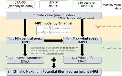
As will be discussed later, MPS assumes typhoon track, so-called the worst-case typhoon track, considering the shape of bay in advance. Therefore, there are bays where the worst-case typhoon track assumption cannot be applied when referring to historical typhoon track records. The worst-case typhoon track assumption is not mainly applicable to the Sea of Japan side in Japan and some bays in East Asia. The following discussion focuses on representative bays in East Asia and the Pacific side of Japan, where the MPS concept applies.

2.1. Theoretical framework

2.1.1. Maximum potential intensity (MPI)

The MPI is widely used to estimate the maximum intensity of a TC. Two main theories for estimating the MPI have been proposed by Emanuel (1988) and Holland (1997), and we use the former theory proposed by Emanuel (1988) here. The MPI theory uses convective available potential energy (CAPE) and sea surface temperature (SST) as the main explanatory variables and does not require any arbitrary parameters for adjustment. Based on the MPI theory (Emanuel 1988; Bister and Emanuel 2002), the Carnot cycle is assumed for an axis-symmetric TC, and the TC’s maximum development limit in a given environmental field is expected to be the ideal lower limit of central pressure (i.e. minimum central pressure) of a TC. The maximum possible wind speed, $V_m$, and minimum possible pressure (which occurs at the radius of maximum wind speed), $P_m$, are estimated using CAPE, SST, vertical profiles of atmospheric temperature and humidity (i.e. for deriving CAPE), and sea level pressure (SLP) as

(1) ${V_m}^2=\frac{C_k}{C_D}\frac{T_{\mathrm{s}}}{T_0}\left(\mathrm{C}\mathrm{A}\mathrm{P}{{\mathrm{E}}_m}^{\ast }-\mathrm{C}\mathrm{A}\mathrm{P}{\mathrm{E}}_m\right)$(1)

(2) $R_d{T}_s\mathrm{l}\mathrm{n}\frac{P_{env}}{P_m}=\frac{1}{2}{V_m}^2+\left(\mathrm{C}\mathrm{A}\mathrm{P}{\mathrm{E}}_m-\mathrm{C}\mathrm{A}\mathrm{P}{\mathrm{E}}_{\mathrm{e}\mathrm{n}\mathrm{v}}\right)$(2)

where T_s is the SST, $T_0$ is the tropopause temperature, $P_{env}$ and $\mathrm{C}\mathrm{A}\mathrm{P}{\mathrm{E}}_{\mathrm{e}\mathrm{n}\mathrm{v}}$ are the environmental background SLP and CAPE, $C_D$ and $C_k$ are the momentum and heat exchange coefficients at the sea surface (respectively), and $R_d$ is the gas constant for dry air. The ratio of $C_D$ to $C_k$ is defined 0.9 following Emanuel (2021) and see the detail of the other definitions in Emanuel (1988), Bister and Emanuel (2002) and Mori et al. (2021b). The superscript * denotes the saturated air condition, and the same subscript m is used to denote the value evaluated at the radius of maximum wind speed. While these equations are primarily a function of CAPE and SST, CAPE_m* and CAPE_m depend on the pressure and, therefore, Eq. (1)(1) ${V_m}^2=\frac{C_k}{C_D}\frac{T_{\mathrm{s}}}{T_0}\left(\mathrm{C}\mathrm{A}\mathrm{P}{{\mathrm{E}}_m}^{\ast }-\mathrm{C}\mathrm{A}\mathrm{P}{\mathrm{E}}_m\right)$(1) and (2(2) $R_d{T}_s\mathrm{l}\mathrm{n}\frac{P_{env}}{P_m}=\frac{1}{2}{V_m}^2+\left(\mathrm{C}\mathrm{A}\mathrm{P}{\mathrm{E}}_m-\mathrm{C}\mathrm{A}\mathrm{P}{\mathrm{E}}_{\mathrm{e}\mathrm{n}\mathrm{v}}\right)$(2) ) must be iterated until $P_m$ converges. In addition, the vertical air temperature gradient is generally more stable due to global warming and suppresses TC generation numbers in the future. On the other hand, the maximum intensity becomes stronger when the SST is higher by global warming (e.g. Yoshida et al. 2017). Future TC characteristic changes are generally balanced between two opposing effects of increasing atmospheric stability and SST.

In this study, the MPI is used as a proxy to assess long-term changes in future TC intensity and as an input for the MPS model. More specifically, the MPI estimates the maximum developmental intensity of a TC based on background environmental conditions. However, it is unclear what relationship or bias this has with TCs that are represented by GCMs. For this reason, we compare future changes (in TC intensity) between the derived MPI and TCs in GCMs, using a robust, large-ensemble climate-change projection dataset (see Section 3). Furthermore, this same large-scale climate ensemble (such as the d4PDF ensemble) can be used to confirm the statistical stability of the estimated maximum as represented by the TC intensity by MPI.

2.1.2. Maximum potential storm surge (MPS)

In the MPS model, storm surge is regarded as a linear combination of pressure-induced and wind-induced effects, which are evaluated independently (Mori et al. 2021b). Here we briefly describe the basic assumptions used and outline the MPS model. First, it is assumed that the minimum central pressure, $P_{min}$, is equivalent to the minimum possible pressure obtained from the MPI (i.e. $P_m$); in addition, the definition of $V_m$ in time and height from the ground is not clear, and we regard $V_m$ is defined 1-minute averaged at 10 m height from mean sea level. The maximum wind speed, $V_{max}$, is derived using a gradient wind model with an empirical relation between Pm and TC radius (see Mori et al. 2021b), which uses a conversion coefficient to take into account the effects of the super-gradient wind (Fuji and Mitsuta, 1986) in the interior of the boundary layer, to modify the maximum possible wind speed obtained from the MPI (i.e. $V_m$). Although there is several choices of the pressure-wind relationship based on the parametric representation (e.g. Knaff and Harper, 2010), we use the super-gradient wind model for simplicity. Second, a worst-case storm surge scenario is assumed to occur in each bay analyzed. Here, the TC translational effect on wind speed (longwave speed in the bay) has been added to the wind speed input in the model. Third, the wave-induced sea surface change (i.e. radiation stress effects) is not considered for simplicity.

A pressure-induced surge will occur when the translation speed of the TC, $V_T$, is similar to the longwave velocity C in the bay. Here, we assume that any resulting pressure wave will travel from offshore to onshore along the major axis of the bay. For simplicity, we use a one-dimensional pseudo channel with a constant-cross-sectional bathymetry h = h(x) which varies along the major axis of the bay ($x$) from onshore ($x=0$) to offshore ($x=x_{end}$). We also assume that the pressure wave, ${\zeta }_p$ can be given by the following equation,

(3) ${\left.{\zeta }_p\right|}_{V_T\to C}=\frac{1}{{\rho }_{\mathrm{w}}g}\left\{\varphi \left(t-\frac{x}{V_T}\right)-\frac{x}{2C}\varphi \prime \left(t-\frac{x}{V_T}\right)\right\}$(3)

where ${\rho }_w$ is the density of seawater,$g$ is the acceleration of gravity, and $\varphi =\varphi \left(x\right)$ is the horizontal pressure profile. Then, substituting Myers’ pressure distribution P into this equation, a maximum value of the pressure-induced surge ${\zeta }_p$ can be obtained. Correspondingly, a maximum wind-induced surge ${\zeta }_w$ can also be derived for the pseudo channel, which assumes a worst-case scenario with the wind direction aligned with the major axis (from offshore to onshore). By considering the balance between the sea surface and bottom friction stresses, the sea surface elevation ${\zeta }_w$ from a wind-induced surge can be calculated as,

(4) ${\zeta }_w=K_{rev}\cdot \frac{{\rho }_a}{{\rho }_{\mathrm{w}}g}\cdot U^2$(4)

(5) $K_{rev}=K\cdot \hspace{0.17em}0x_{end}\frac{1}{h\left(x\right)}dx$(5)

where ${\rho }_a$ is the air density, $K$ and $K_{rev}$ are bathymetric and empirical coefficients (respectively), $U$ is the wind speed at 10 m height, and $U$ is linearly combined by $V_m$ and $V_T$. Finally, the MPS can be expressed as a linear combination of the wind-induced and pressure-induced surges as ${\zeta }_p+{\zeta }_{\mathrm{w}}$ neglecting interactions between wind and pressure-induced surges (see Figure 1 again for an outline of the MPI-MPS framework).

The coefficient $K$ varies depending on the bathymetry h(x) and needs to be optimized for each bay. A series of storm surge simulations using the ADvanced CIRCulation (ADCIRC) model were used as a reference for the calibration; the top five extreme storm surge cases from the model were used to estimate an average bay-specific $K$, as noted in Mori et al. (2021b). The ADCIRC simulations were performed on an unstructured grid, and the computational domain covers a globe composed of 2.4 million grid cells with variable spatial resolutions ranging from 2 km (nearshore) to 25 km (offshore). In addition, the model was forced with reanalysis data (see Shimura et al. 2022) – hourly sea surface winds (U10) and sea level pressure (SLP), and monthly sea ice concentrations derived from 150-year continuous scenario run and a 55-year atmospheric reanalysis dataset (see Section 2.2 for details). Therefore, a total of 205 years of simulations were used to calibrate $K_{rev}$. It should be noted that astronomical tides are not considered in this study. Furthermore, comparisons between the dynamic storm surge model and the MPS model are performed using the following steps for each bay:

(1) Select storm surge events larger than 1 m;

(2) Retrieve the minimum central pressure $P_{min}$ and the maximum wind speed $V_{max}$ from the selected TCs in step 1;

(3) Feed $P_{min}$ and $V_{max}$ into the MPS model;

(4) Compare the maximum surge heights between the dynamic and MPS models.

The application of the MPS model will be discussed in Section 4.

2.2. Numerical setup and target area

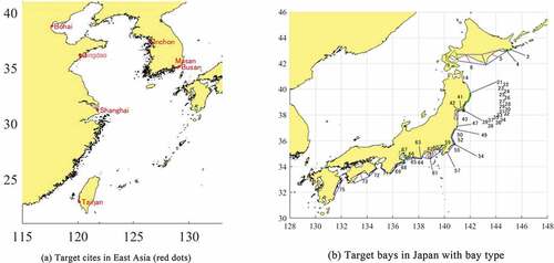
A previous study by Mori et al. (2021b) analyzed three major bays in Japan: Tokyo Bay, Ise Bay, and Osaka Bay. Here, we calculate the MPS for seven major bays in East Asia, considering the bay shape and hazard exposure as population and asset. In addition, we also calculate the MPS for 51 bays along the Pacific coast of Japan. We have omitted coasts along the Sea of Japan since the MPS method assumes a worst-case TC track scenario for each bay. It is difficult to apply the method from a meteorological point of view (i.e. TCs approaching from the north). Figure 2 shows the locations of the selected cities or bays for (a) East Asia and (b) Japan. Details of the bay geometries have also been added to Figure 2b; red lines indicate the major axis of the bays, and the colored trapezoids indicate the bay boundaries and type (blue, open; green, closed). The targeted cities in Figure 2a correspond to Jiaozhou Bay around Qingdao, Yangtze River Estuary around Shanghai, Bohai Sea around Bohai, and Jinhae Bay around Masan, respectively. In addition, the Japanese bays have been enumerated from the north to the south, as shown in Figure 2b.

Figure 2. Map of target coastal cities or bays for projection. Colored lines in panel (b) describe bay type: red, major axis; blue, open bay; green, closed bay (see Figure 13 for bay names).

A bathymetry profile is required to estimate the wind-induced surge effect in Eq. (4(4) ${\zeta }_w=K_{rev}\cdot \frac{{\rho }_a}{{\rho }_{\mathrm{w}}g}\cdot U^2$(4) ), and different datasets were used for East Asia and Japan. For East Asia, we used the General Bathymetric Chart of the Oceans (GEBCO; 2020); it has a grid width of 15 arcsec (about 470 m) worldwide and is enough to estimate the mean cross-sectional depth of the seven large-scale bays selected (Figure 2a). For Japan, we used the M7000 series coastal bathymetry data by the Japan Hydrographic Association (2021). The higher resolution M7000 data was converted from meshless point-values to gridded averages using bilinear interpolation; the interpolated data is five arcsec (about 150 m), which is also enough to represent the bathymetries of the smaller and intricate bays. For stability, we have limited the water depths from 2 m to 500 m in the MPS calculations in order to ensure that the hypothetical TC translation speeds do not become too fast in bays with very deep water (to match the longwave velocity).

For three open bays in East Asia – Bohai, Shanghai, and Tainan, it is difficult to define the bay mouth because either the depths are extremely shallow or the bays are too wide. Therefore, the optimal value of $x_{end}$ in Eq. (5)(5) $K_{rev}=K\cdot \hspace{0.17em}0x_{end}\frac{1}{h\left(x\right)}dx$(5) is searched by setting the initial value to 60 km provisionally and determining the optimal value that minimizes the root mean square error (RMSE) of the storm surge estimation.

Environmental conditions (SST, vertical profile of air temperature and air humidity, and SLP) are necessary to calculate the MPI fields and analyze the MPS for present and future climates. Therefore, we used monthly mean climate values from three different datasets for the climate change impact assessment. These datasets are based on simulations from the MRI-AGCM3.2 H, a 60 km atmospheric global climate model (AGCM) developed by the Meteorological Research Institute of the Japan Meteorological Agency (Mizuta et al. 2012). Systematic differences (biases) exist in climate projection data when compared to atmospheric reanalysis data. Bias correction for individual scalar variables is possible. However, there is no established method for bias correction of multivariate, three-dimensional data, correlated values (e.g. SST and air temperature) It is also quite difficult to apply bias corrections for three dimensional multivariate keeping dynamical and thermodynamic relationships such as those used here. Therefore, in the following sections, no bias correction is made for climate projection data, and the data is evaluated using the values as they are.

The first dataset, HighResMIP (Haarsma et al. 2016; Shimura et al. 2022), is a series of 150-year continuous scenario projections (hereafter referred to as the 150-year scenario); the present climate experiment (named HPD) covers the period 1950–⁠2014, while the future climate experiments (named HFD) cover the period 2015–2099 and use the RCP2.6 and RCP8.5 forcing scenarios. RCP2.6 is a scenario to keep global warming likely below 2°C at the end of the 21^st century, and RCP8.5 is very high greenhouse gas emission scenario that exceeds 4°C at the end of the 21^st century. In addition, the present experiments HPD use historical SSTs as a lower boundary condition for the MRI-AGCM3.2 H, while the future experiments HFD use ensemble averages of projected SSTs from the CMIP5 experiments. Furthermore, it should be noted that the present experiments HPD were generated using four different initial perturbations (m00-03) to estimate internal uncertainty, but the future experiments HFD run were only generated for a single member of each RCP scenario.

The second dataset we used was the Database for Policy Decision-Making for Future Climate Change (d4PDF/d2PDF). This large ensemble dataset was mentioned in the introduction and created to help assess changes in climate extremes (Mizuta et al. 2017; Ishii and Mori 2020). This dataset, denoted the d4PDF ensemble hereafter, was generated using the same model (MRI-AGCM3.2 H) for the scenario projection but was forced with different future climate conditions. Although each ensemble member for both the present and future climate conditions was integrated for 60 years, the present climate condition in the d4PDF ensemble dataset uses SST observations as the lower boundary condition, while the future climate condition uses six different SST warming patterns based on the CMIP5 experiments. Additionally, the six future SST patterns were perturbed with 15 initial ensembles, giving a total of 90 ensemble members (d4PDF ensemble present has 100 members). The present climate SSTs for the d4PDF ensemble include observed warming trends. On the other hand, the future SSTs of d4PDF ensemble are based on the +2 K or +4 K warmer global mean SSTs with the addition of natural variability derived from observations detrended to the monthly SST patterns of six different climate models from the CMIP5 RCP8.5 experiments (CCSM4, GFDL-CM3, HadGen2-AO, MIROC5, MPI-ESM-MR, and MRI-CGCM3) (see Mizuta et al. 2017 in detail). Each SST trend was rescaled by a multiplying factor that forces the MRI-AGCM3.2 to simulate a global-mean surface air temperature equivalent to each warming level (see Mizuta et al. 2017; Ishii and Mori 2020); therefore, a global mean of +2 K and +4 K conditions are added exactly to the present climate condition. Aside from the significant difference in the number of runs, the present experiments of the d4PDF ensemble and the 150-year scenario are basically the same, except that the SST values for the latter follow the guidelines according to the HighResMIP experiment.

The third dataset we used was for validation purposes and comprised of a 55-year long-term atmospheric reanalysis (JRA-55; Kobayashi et al. 2015) and SST observational (COBE-SST; Centennial in-situ Observation-Based Estimates of the variability of SST and marine meteorological variables; Ishii et al. (2005)) data by the Japan Meteorological Agency (JMA). This reanalysis data is simply referred to as the JRA-55 reanalysis hereafter.

2.3. MPS optimization and validation

The MPS model needs to calibrate the empirical coefficient $K_{rev}$ (or $K$) in Eq. (5)(5) $K_{rev}=K\cdot \hspace{0.17em}0x_{end}\frac{1}{h\left(x\right)}dx$(5) for the wind-induced surge for each bay. The wind-induced surge coefficient $K_{rev}$ is dependent on the bathymetric coefficient $K$, which is given by the cross-sectional bathymetry described in the previous section and can be calculated using a reference storm surge simulation conducted by a dynamic model. The calibration needs a variety of storm surge simulations, including a worst-case track simulation for any TC condition. We used a series of 150-year scenario global storm surge projection results that consider climate change (Shimura et al. 2022) and were calculated using the unstructured-grid ADCIRC model (Pringle et al. 2021). The calibration of MPS requires extreme storm surge events, and the more simulations of the teaching data, the better. Therefore, we added other previous storm surge simulations (Yasuda et al. 2014), which use the SuWAT model (Surge-Wave-Tide coupled model) by Kim, Yasuda, and Mase (2010) for Osaka and Ariake Bays in Japan.

Based on the previous study (Mori et al. 2021b), the RMSEs of the MPS model to the dynamic model for the worst-case track are 0.05 m, 0.11 m, and 0.03 m for Tokyo Bay, Osaka Bay, and Ise Bay. Following the previous study, we applied the calibration MPS for six major bays in East Asia and Japanese bays along the Pacific coast. Figure 3 illustrates the calculation procedure used for calibrating the wind-induced surge constant $K_{rev}$. ADCIRC calculations for the present and future climate conditions were performed for a total of 205 years seamlessly (Shimura et al. 2022) and give enough length and quality of storm surge events to calibrate the MPS model over the entire domain along the Pacific. The ADCIRC simulations were analyzed to obtain the peak surge heights, peak time, and TC approaching angles for each bay. There is a time lag between when a TC is closest to the targeted bay and when the maximum storm surge occurs. We have set this peak time difference to 24 hours in order not to remove any cases of large TCs passing far from the bay. Additionally, in the ADCIRC simulations, semi-diurnal water level fluctuations due to atmospheric oscillations due to diurnal changes in the atmosphere were clearly observed in the Yellow Sea and the East China Sea due to the wide and shallow water environment in compassion the other area (e.g. Dai and Wang 1999). Thus, these semi-diurnal oscillations were excluded using Fourier analysis in those seas, which include Incheon Bay. Based on the core data from the ADCIRC simulations, the empirical coefficients $K_{rev}$ for the wind-induced surge were calibrated to minimize the RMSE of peak surge heights for selected cases with a wind angle within $\pm$ 45° to the major bay axis of each bay. In the case of Tokyo Bay and Ise Bay, the simplified model by Eq. (3)(3) ${\left.{\zeta }_p\right|}_{V_T\to C}=\frac{1}{{\rho }_{\mathrm{w}}g}\left\{\varphi \left(t-\frac{x}{V_T}\right)-\frac{x}{2C}\varphi \prime \left(t-\frac{x}{V_T}\right)\right\}$(3) and (5(5) $K_{rev}=K\cdot \hspace{0.17em}0x_{end}\frac{1}{h\left(x\right)}dx$(5) ) tends to overestimate the combined surges. Therefore, the minimum depth was defined as 10 m, and the integration endpoints of Eq. (5)(5) $K_{rev}=K\cdot \hspace{0.17em}0x_{end}\frac{1}{h\left(x\right)}dx$(5) were modified carefully to minimize the RMSE of peak surge heights. 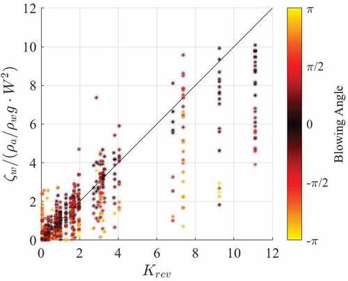The calibrated $K_{rev}$ gives a RMSE less than 0.25 m in all bays except for Matsushima (0.32 m), Ise Bay (0.53 m), and Tokyo Bay (0.50 m). Figure 4 shows the characteristics of the wind-induced surge coefficient $K_{rev}$ for all the bays in Japan. The horizontal axis shows the estimated $K_{rev}$; the vertical axis shows the estimated wind-induced surge ${\zeta }_w$ normalized by the given wind speed W, and the color indicates the wind angle alignment with the bay (zero corresponds to the inward major-bay-axis direction). The optimized results follow the line with the unit slope, and the estimated wind-induced surge ${\zeta }_w$ for selected cases with a wind angle within $\pm$ 45°, are generally located near this line. Thus, the calibration of $K_{rev}$ for the worst track has been achieved. It should be noted that Figure 4 includes $K_{rev}$ for all of the targeted bays and indicates its range; the bays with large $K_{rev}$ appear to be sensitive to the wind-induced surge, while the bays with smaller values less so.

Figure 3. Flow chart for estimating wind-induced surge coefficient ($\mathrm{R}\mathrm{i}\mathrm{y}\mathrm{a}\mathrm{d}\mathrm{h}$) and relation with MPS model.

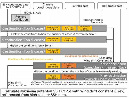
Figure 4. Relationship between wind-induced surge coefficient ($K_{rev}$) and estimated wind-induced surge (${\zeta }_w$) normalized by wind speed. Wind direction relative to bay is indicated by color bar.

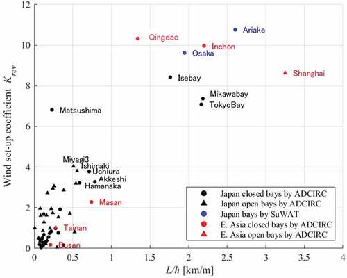
The empirical coefficient $K_{rev}$ expresses the local surge amplification characteristics of each bay. It is interesting to analyze the relationship between the empirical coefficient and bay geometries. In Figure 5, a scatter plot is shown between $K_{rev}$ and the bay length-to-depth ratio L/h for all the bays. The different colors indicate the different regions or different dynamical storm surge models used for calibration. In addition, the circle and triangle marks indicate closed/semi-closed or open bay shapes, which are based on the maximum bay width-to-bay mouth width (offshore) ratios. Notice that a larger value of $K_{rev}$ indicates stronger wind-induced surge effects for the same wind speed, and a larger value of L/h indicates a longer and shallower bay shape in the major axis direction (in a simple rectangular bay geometry, the wind-induced surge is proportional to L/h as shown in equations (4)(4) ${\zeta }_w=K_{rev}\cdot \frac{{\rho }_a}{{\rho }_{\mathrm{w}}g}\cdot U^2$(4) and (5(5) $K_{rev}=K\cdot \hspace{0.17em}0x_{end}\frac{1}{h\left(x\right)}dx$(5) )). Except for Shanghai, which has a very shallow open bay, most of the bays with larger $K_{rev}$ values tend to be closed/semi-closed. Also, the effect of long-period bay oscillations (e.g. seiche, tidal sub-oscillation) on storm surge is considered to be strong since this effect is indirectly incorporated into the calibration process due to the training data used by the dynamic storm surge model. Aside from Matsushima, bays with an estimated $K_{rev}$ coefficient larger than 6 show significant changes in storm surge and will be discussed in the following section. In addition, bays with a large value of $K_{rev}$ will have a large maximum wind-induced surge, resulting in a potentially large storm surge. Therefore, all the bays in Figure 5 which have a large value of $K_{rev}$ – Tokyo Bay, Osaka Bay, Ise Bay, Ariake Sea, Incheon, Qingdao, and Shanghai – are expected to have potentially large projected future changes due to climate change. This will also be analyzed in the next section.

Figure 5. Relationship between bay length-depth ratio and wind-induced surge coefficient. Bay region and type are indicated by color (Japan: black, brown and blue; East Asian: red) and shape (closed: circles; open: triangles).

3. Biases and future changes in the MPI

Our analysis mostly concentrates on variations of the MPI in the western North Pacific Ocean (WNP). For simplicity, some of the analyses use monthly mean MPI data spatially averaged over the TC-prone WNP (defined here as 10–40°N and 100–180°E) and focus on the four most active TC months (July through October; hereafter referred to as TC season). Since it is not clear what relationship or bias the MPI has with TCs that are represented by GCMs, we also compare present and future changes (in TC intensity) between the derived MPI and TCs in GCMs, using the JRA-55 reanalysis (present) and d4PDF ensemble (future) datasets. TCs were picked up from the projections based on TC tracking methods by Webb, Shimura, and Mori (2019). The characteristics and validation of modeled TCs by MRI-AGCM have been discussed by Yoshida et al. (2017).

3.1. Biases in the MPI

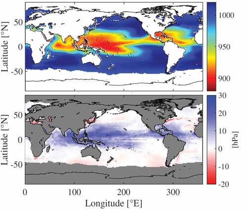
Before analyzing future changes in the MPI, we will discuss biases in the MRI-AGCM for the present climate conditions. Figure 6 (top) shows the monthly mean MPI for September for the 150-year scenario, as well as Figure 6 (bottom) the spatial distribution differences with the JRA-55 reanalysis dataset. We can see that the September monthly mean MPI from the 150-year scenario dataset decreases monotonically off the Pacific coast of East Asia from the equator to the north. It has a value of about 940–950 hPa near the southern coast of Japan. Additionally, differences between the two MPI monthly means indicate that the 150-year scenario tends to be weaker than the JRA-55 reanalysis over most Pacific oceans. The differences between the two MPIs are about ±10 hPa, with a positive bias (underestimation) from the equatorial region to the southern coast of Japan, and a negative bias (overestimation) north of this latter region. Since the SSTs for both datasets are climatologically equivalent, the main cause of this bias seems to be differences in the vertical distributions of air temperature; the JRA-55 reanalysis uses data assimilation for the vertical distribution of atmospheric temperature and other variables, while the d4PDF ensemble does not since it performs climate calculations.

Figure 6. Monthly mean MPI for period-averaged in September (top: present climate in 150-year scenario, bottom: difference between 150-year scenario and JRA-55).

3.2. Future changes in the temporal MPI in the WNP

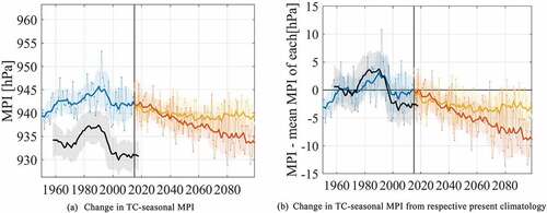
In Figure 7, time series of (spatially) basin-averaged MPI are shown for the WNP that were calculated using the 150-year scenario and JRA-55 reanalysis datasets during the TC season. In order to understand the interannual characteristics of the MPI, TC seasonal means are shown with their 10-year moving averages’ respective standard deviations (STDs). Figure 7a shows the change in the TC seasonal MPI for the HPD four-ensemble-mean (blue), HFD RCP2.6 (yellow), HFD RCP8.5 (orange), and JRA-55 reanalysis (black) datasets, while panel (b) shows the change from each of the respective present climate conditions. Figure 7a) reveals a bias in the MPI calculations between the reanalysis and the present climate runs (HPD). Compared with the MPI in the reanalysis run, the present climate run shows higher MPIs (i.e. weaker TCs) of about 10 hPa. As mentioned in the last section, the main cause of this bias in CAPE is due to differences in the vertical distribution of atmospheric temperature. Since the SST boundary conditions for the AGCM in the present climate run are basically equivalent to those in the reanalysis run, the major bias in the MPI in the present climate run HPD depends on a bias in CAPE. We did not analyze it in detail due to out of the scope of our study. The bias correction is a future work due to the complexity of the multivariate relationship. Furthermore, the MPI for the 150-year scenario runs shows continuous strengthening trends from the present to the end of the 21^st century; the MPI in the RCP8.5 run shows a monotonically decreasing trend, while the RCP2.6 run stabilizes around the middle of the 21^st century. Future changes in the 10-year moving averages of the (TC seasonal) MPI indicate reductions of −3.5 hPa and −8.9 hPa for the RCP2.6 and RCP8.5 scenarios (respectively) at the end of the century.

Figure 7. Time series comparisons of MPI (basin-averaged over WNP) during TC-season for 150-year scenario and reanalysis datasets. Colors represent different runs; blue: HPD four-ensemble-mean, yellow: HFD RCP2.6, Orange: HFD RCP8.5, and black: JRA-55 reanalysis. Thin lines represent TC-seasonal means while thick lines and shaded regions represent their 10-year moving averages and STD widths, respectively.

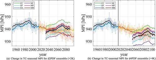
Next, we examine the characteristics of the signal (both biases and future change) found in the MPI from the 150-year scenario by comparing it with the d4PDF ensemble. In Figure 8, the time series of the ensemble mean of each SST cluster in the d4PDF ensemble dataset are compared with the 150-year scenario during the TC season. Similar to Figure 7, the time series show (spatially) basin-averaged MPI for the WNP during the TC season but for the +2 K and +4 K warming conditions. Here, Figure 8 shows that the MPI from the 150-year scenario is generally consistent with the d4PDF ensemble total (ensemble) means (both present and future); additionally, it also shows that interannual changes in the MPI are relatively large in the d4PDF ensemble dataset, as well as differences among the different future SST conditions. Based on the description paper of d4PDF (Mizuta et al. 2017), HA (HadGEM2-AO), MP (MPI-ESM-MR) and MR (MRI-GCM3) are El Niño–like pattern of SST change, but the others are typical SST warming in the eastern equatorial Pacific. The future projection based on El Niño–like pattern of SST shows similar MPI but the others are scattered. On the other hand, large peaks are observed around 40 years (1990 or 2070) from the start of the projection in the d2PDF/d4PDF ensemble dataset. This is also seen in the results of JRA55, and seems to be one of the major decadal variations. In addition, compared with the 10-year moving average of the JRA-55 reanalysis MPI in Figure 7a, the d4PDF ensemble MPI is closer to the results of the 150-year scenario during the present climate, indicating that there is a similar bias between the d4PDF ensemble and the 150-year scenario as described above.

Figure 8. Time series comparisons of MPI (basin-averaged over WNP) during TC-season for 150-year scenario and d4PDF ensemble datasets. Blue yellow, and Orange lines and shadings for 150-year scenario runs are same as in Figure 6. In d4PDF ensemble dataset, colors in legend represent future SST-cluster ensemble means (not moving averages as in Figure 6), while black lines and gray shadings represent present and future total ensemble means and spreads of d4PDF ensemble datasets, respectively.

3.3. Future changes in the spatial MPI in the WNP

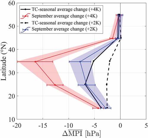
In order to examine future changes in the MPI in the WNP in more detail, we analyzed the latitudinal characteristics of future changes in the mean (total ensemble) MPI of the d4PDF ensemble dataset between the TC season and September. Figure 9 shows the results of the zonally averaged MPI in 10° latitudinal bands for the full WNP (extended to cover 10–60°N here). For September, the month with the largest future changes, the maximum future changes in the MPI are observed in the 30–40°N band where the East Asia countries are located, with average changes of −7.8 hPa and −16.5 hPa for the +2 K and +4 K warming conditions (respectively). These values are approximately three times larger than the TC seasonal mean future changes for the same latitudinal band. Therefore, future changes in TC intensity in the WNP strongly depend on both month and latitude. These results are consistent with the previous study of the MPI with the CMIP5 experiments (Mori et al. 2021b). Additionally, any future changes in the MPI at higher latitudes may lead to a northward expansion of the developmental limit for a TC in the WNP, which necessitates a more detailed analysis (e.g. Kossin, Emanuel, and Camargo 2016).

Figure 9. Zonal distribution of future changes in MPI (temporally and spatially averaged in 10° latitudinal bands over WNP) for d4PDF ensemble dataset. Red and blue lines (shadings) represent total ensemble means (spreads) during September for +4 K and +2 K future conditions, respectively; solid black and dashed lines represent total ensemble means in September for +4 K and +2 K future conditions, respectively.

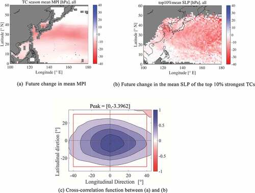
In typical time-slice experiments of 20 to 30 years, the projection period is too short to effectively use the MPI to evaluate future changes in the maximum intensity of a TC. In addition, time-slice experiments also typically include a warming trend, so the projections are non-stationary. Since the MPI theory only relies on background environmental conditions, the first problem can be overcome by using a large ensemble dataset; however, the accuracy and any biases of future changes will still need to be verified. Figure 10 shows the future changes in the WNP in the mean MPI for all d4PDF ensemble members (+4 K scenario) during the TC season and the mean minimum central pressure of the top 10% strongest TCs (central pressure at maximum development) as directly extracted from the d4PDF ensemble members (denoted SLP10%). The future changes in the mean MPI of the TC season and future changes in the SLP10% of the GCM TCs with the top 10% intensity are similar in value (−15% approximately) but are different spatial distributions. These results suggest that the maximum potential TC intensity represented by the MPI is equivalent to the top 10% of the intensity in the model. In the Northwest Pacific results shown in Figure 10, MPI and SLP10% TC is weakly correlated, and it’s the correlation coefficient is 0.5 approximately. The correlation coefficient is highest when the SLP10% TC distribution is shifted 3.4 degrees to the south. Both spatial distributions show significant future changes in the north-south direction, which confirms the latitudinal dependence of the mean MPI of TC season and the future changes of GCM TCs as well as the future changes of MPI in the latitudinal direction shown in Figure 9. While the spatial distribution of MPI sharply increases or decreases in a latitudinal direction, the spatial distribution of SLP10%TC has a much larger north-south spread. This latitudinal difference is interpreted/evaluated as a spatial bias of the TC to the maximum development as assessed by the MPI.

Figure 10. Future changes (+4 K) in mean MPI of TC season and SLP of strong TCs calculated by d4PDF ensemble and their two-dimensional cross-correlation (1.25X1.25-degree grid). (a) Future change in mean MPI, (b) Future change in the mean SLP of the top 10% strongest typhoons, (c) Cross-correlation function between (a) and (b) (red box indicates significant area for cross-correlation analysis).

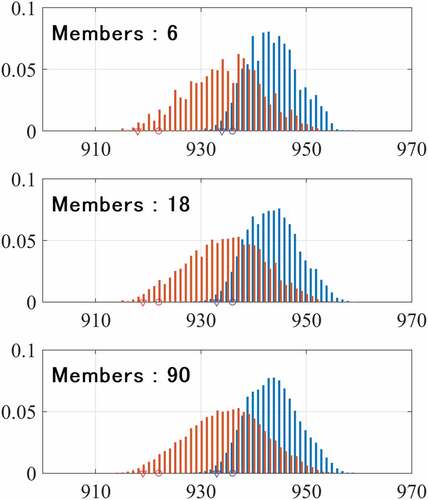
Due to a large number of ensembles, results from the d4PDF ensemble dataset can be used to discuss the MPI occurrence probabilities directly. Here, we compare discrete probability distributions of the mean (total ensemble) MPI in the typhoon-prone WNP for different ensemble sizes. Figure 11 shows changes in the probability distributions of the (spatially) basin-averaged MPI for the WNP that were calculated using the d4PDF ensemble dataset with an increasing number of ensemble members during the TC season. Since the typhoon months are defined as July through October, there are 120 months of average MPI for each member. An equal number of members were selected from each SST cluster in the future climate condition. The blue and red colors represent the present and +4 K future climate conditions (respectively), while the triangles and circles on the horizontal axis represent the top 1^st and 5^th MPI percentiles (respectively). Figure 11 shows that the MPI method does not require a large number of ensembles, but the distribution becomes smoother as the number of ensembles increases. By comparing the typical percentile values, an ensemble with as few as six members can produce results almost as good as the larger ensembles. Since Figure 8 shows a large variability among the different future SST clusters, it is ideal to use enough future SST variations from AOGCMs rather than increasing the number of initial ensemble members.

Figure 11. Comparison of probability density distributions of MPI (basin-averaged over WNP) for different ensemble sizes during TC-season of d4PDF ensemble dataset. Blue and red colors represent present and +4 K future climate conditions, respectively; triangles and circles represent top 1^st and 5^th percentiles, respectively.

4. Future changes in the MPS

Since the statistical characteristics of the MPI from the d4PDF ensemble and the 150-year scenario datasets are clear, we have used the 150-year scenario to perform the MPS analyses for the targeted bays in East Asia and Japan. The MPS are calculated using the monthly mean MPI values of the four nearest grid cells (central pressure and maximum wind speed), as documented in Figure 1. A sample spatial distribution of the MPI is shown in Figure 6 for the September monthly mean over the dataset period; since the MPI field is smooth, the differences between the average and any of the nearest MPI gridded neighbors depend on the latitude. It should be noted that MPI of 150-year scenario datasets has a bias that is overestimated and underestimated biases in the south and north around 30 degrees north latitude, respectively. Here, we will analyze each bay’s long-term changes in the mean MPS during the TC season (from July to October).

4.1. Future changes in the MPS at major bays in East Asia

In Figure 12, time series of the MPS are shown for the East Asian bays. As in Figure 7, TC seasonal means are shown with their 10-year moving averages and respective STDs for the present climate HPD four-ensemble-mean (blue), future climate HFD RCP2.6 (yellow), and future climate HFD RCP8.5 (orange) runs. Figure 12 shows that the MPS will increase in the future for most East Asian bays. As with future changes in the MPI (but with an inverse trend), the MPS in the RCP8.5 run shows a monotonically increasing trend, while (the MPS in) the RCP2.6 run increased initially but stabilize around the middle of the 21^st century.

Figure 12. Time series comparisons of MPS for East Asian cities during TC-season for 150-year scenario dataset. Colors represent different runs: blue, HPD four-ensemble-mean; yellow, HFD RCP2.6; and Orange, HFD RCP8.5. Thin lines represent TC-seasonal means while thick lines and shaded regions represent their 10-year moving averages and STDs, respectively; gray line represents maximum storm surge by dynamic model.

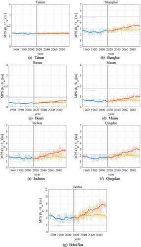
Furthermore, the gray horizontal line in Figure 12 shows the maximum storm surge from the dynamic storm surge simulation used for calibrating the MPS model. The maximum MPS (present and future) exceeds the dynamically simulated maximum storm surges except at Shanghai, Busan, and Masan. Since the MPS method estimates the maximum possible value, the MPS should be higher than (but within range of) the maximum values of the dynamical model simulations. Thus, the overestimation of the MPS for Shanghai, Busan and Masan indicates that the $K_{rev}$ value needs to be reduced, while underestimating the Bohai Sea indicates the opposite. There are several reasons for the difference between the MPS and the model maximum. First, $K_{rev}$ value may not have been estimated properly by the calibration process. This is the case for Masan, which has a more complex bay shape, and Shanghai, which has a wide and shallow bay shape than assumed in the MPS framework. On the other hand, based on the relationship between L/h and $K_{rev}$ in Figure 5, the three bays are not an outlier to other bays. Therefore, it is not the main cause of the error. Second, the model maximum estimate may be missing events, and a strong typhoon may not have passed over the worst-case track. Third, input TC information-related error, the bias of MPI, may cause the difference. However, we do not know the detailed source of error to optimize the results for these three cities at the moment, and more detail of calibration is necessary with more teaching datasets for these bays. Overall, though the results are generally consistent; however, further optimization is needed for some bays, especially open ones.

4.2. Future change in the MPS along the Pacific coast of Japan

Although there are many long-term assessments of storm surges for specific bays and periods in Japan, few comprehensive studies cover wide areas or conduct a nationwide analysis with consistent forcing (e.g. Yasuda et al. 2014). The advantage of the MPI-MPS framework is a low-cost calculation with a consistent climatological approach that uses monthly environmental values and is based on the maximum possible assumption. Here, we focus on the future projected changes in the MPS along the Pacific coast of Japan (using the 150-year scenario dataset).

First, we analyzed the statistical distributions of the MPS in the Pacific Japanese bays during the TC season (using the 150-year scenario dataset). In Figure 13a, a box plot shows the quartile distributions (medians, white dots; lower and upper quartiles, solid boxes; 0^th and 100^th percentiles, whiskers; and outliers, colored dots) of the MPS in each bay for the present climate HPD four-ensemble-mean (blue), HFD RCP2.6 (yellow), and HFD RCP8.5 (orange) runs. There are positive changes in the (MPS) quartiles for most of the bays, with larger increases in the higher global warming scenario (RCP8.5). As in Figure 12 and Figure13a, the gray lines indicate the maximum storm surge from the dynamic storm surge simulations (ADCIRC and SuWAT), which generally coincide with the upper quartiles of the box plots at many of the bays. This indicates the consistency of the MPS assumption with the dynamic storm surge model. Basically, the storm surge height by the MPS should be higher than the dynamic storm surge simulation. Comparing the results of the calibrated MPS with the teaching dataset (i.e. dynamic model), the results of the dynamic storm surge simulation should not exceed the results of the MPS. This is an important indicator for the calibration and validation results of the MPS in each bay. The overall performance of the MPS model is better for the Japanese bays than the East Asia ones and may be related to the size and shape of the bays. In addition, the MPS spatial distribution along the Pacific coast shows that the median MPS are higher in the southwestern parts of Japan; this can be attributed to the TC tracks.

Figure 13. Distributions of bay-averaged MPS along Pacific coasts of Japan during TC-season for 150-year scenario dataset; bay names and identifiers are listed along horizontal axis (see Figure 2 for locations). Box plot in panel (a) shows medians (white dots), lower and upper quartiles (solid boxes), 0^th and 100^th percentiles (whiskers), and outliers (colored dots); lollipop plot in panel (b) shows means and STDs (large and small respectively). Colors represent different runs: blue, HPD four-ensemble-mean (top only); yellow, HFD RCP2.6; and Orange, HFD RCP8.5. Gray line represents maximum storm surge by dynamic model.

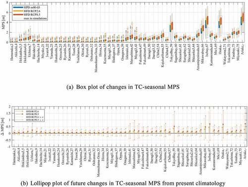
In Figure 13b, a lollipop plot shows the future change in the MPS in the future climate scenarios from the present climatology (∆MPS) during the TC season. The solid circle and triangle markers indicate the TC seasonal means and STDs (respectively). There are two specific characteristics of ∆MPS. First, larger future changes (in the MPS) can be seen in bays with larger MPS in the present climate condition HPD, such as in Tokyo Bay (#59), Ise Bay (#67), Osaka Bay (next to #69), and Ariake Bay (next to #75). Second, larger future changes (in the MPS) are located in the southern and western areas of Tokyo Bay. First, future changes in the MPI in the western part than the northern part of Japan. Additionally, these bays have characteristics occurring large wind-induced surges as shown in Figure 5. Therefore, it can be reworded to the typical intensities and tracks of TCs that make landfall in Japan, which generally approach from the west before turning toward the northeast. The largest projected future changes of the MPS occur in Ariake Bay in the RCP8.5 run, with an additional water level of +0.72 m from the present run HPD. Similar magnitudes of future changes are also projected in Tokyo Bay, Ise Bay, and Osaka Bay, which are long and shallow bays in Japan. On the other hand, the relative differences between the RCP scenarios is generally larger north of 38°N than south. Regarding temporal changes of the MPS, the time series are similar to those of the MPI, as shown in Figure 7. In the RCP2.6 experiment, the peak MPS in most bays (except Hokkaido) is found to occur during the period 2070–2080; likewise, in the RCP8.5 experiment, the MPS increases monotonically toward the end of the century, similarly to the MPI intensity (figures excluded due to a manuscript limitation).

4.3. Sensitivity of the MPS along the Pacific coast of Japan

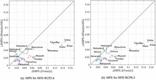
The MPS method estimates the maximum potential storm surge height based on the MPI values expressed in terms of minimum pressure and maximum wind speed. In Figure 14, a scatter plot compares future changes in the MPS (∆MPS) that are divided by two different MPI inputs ∆V_max and ∆P_min in each bay for the (a) HFD RCP2.6 and (b) HFD RCP8.5 runs, respectively. The horizontal and vertical axes are divided by future changes of maximum wind speed (∆V_max) and minimum central pressure (∆P_min) in each bay, respectively. The circles and triangles represent closed/semi-closed and open bays (respectively), while crosses represent simulations conducted by the SuWAT model. Most of the bays in Figure 14 fall below the 1–1 relation shown in the black line, and therefore, the sensitivity of the MPS due to wind speed is greater than that due to atmospheric pressure. Interestingly, the relative ratio of MPS does not appear to be significantly sensitive to the RCP scenario, even though the wind-induced surge is parameterized as a function of the square of wind speed as shown in Eq. (4)(4) ${\zeta }_w=K_{rev}\cdot \frac{{\rho }_a}{{\rho }_{\mathrm{w}}g}\cdot U^2$(4) . In general, the northern bays exhibit relatively greater sensitivity to atmospheric pressure, while the southern bays exhibit greater sensitivity to wind speed. Additionally, the ratio of ∆MPS/∆P_min to ∆MPS/∆V_max tends to decrease in the south, indicating that the sensitivity of wind speed to atmospheric pressure increases southward. Furthermore, the closed/semi-closed bays tend to deviate from the linear relationship more than the open bays. And finally, the bays with the highest sensitivity to wind speed correspond to bays with the largest future changes in the MPS, as shown in Figure 13. These results indicate hot spots for future changes in storm surge.

Figure 14. Sensitivity analysis of future changes of MPS along Pacific coast of Japan (with bay names marked) during TC-season for 150-year scenario dataset; horizontal and vertical axes are MPI ratio to future changes of maximum wind speed and minimum central pressure, respectively. Transition from north to south is indicated by color, while closed and open bays use circles and triangles, respectively.

5. Conclusion

This study evaluates the maximum potential intensity and storm surge of TCs for bays in East Asia and along the Pacific coast of Japan using the MPI-MPS model framework. Future changes of the MPI are analyzed for the WNP using two climate projection datasets generated by the high-resolution MRI-AGCM3.2 H model: 150-year continuous scenario runs (HighResMIP) and large ensemble (d4PDF/d2PDF). Trends and spatial characteristics of future change are evaluated with sensitivity analyses for different global warming scenarios. The following is a summary of the major findings of this study.

1. Empirical coefficients for the wind-induced surge were estimated for seven bays in East Asia and 51 bays in Japan. Shallower and longer bays have larger wind-induced surge coefficients ($K_{rev}$).

2. Interannual changes in the MPI over WNP show a monotonically decreasing trend (increasing TC intensity) at the end of the century. The decreasing (intensifying TC) MPIs at the end of the century are −3.5 hPa and −8.9 hPa for the RCP2.6 and RCP8.5 scenarios (respectively) using the 150-year scenario dataset.

3. Future changes in the MPI are greatest during September in the 30–40°N latitude band of the extended WNP, with average changes of −7.8 hPa and −16.5 hPa for the +2 K and +4 K future conditions (respectively) using the d4PDF ensemble dataset.

4. Future changes in the MPS were projected, and it was confirmed that changes in the MPS are larger in bays where large storm surge events have occurred in the past.

5. Sensitivity analysis results show that the MPS sensitivity to wind speed is greater in southwestern Japan and tends to be larger in closed/semi-closed bays.

These results suggest that the future trends of the maximum storm surge in East Asia can be understood by targeting bays in hot spots.

This paper applied a framework for MPI and MPS derived from climate values without using extreme typhoon projections in GCMs, which are subject to large statistical uncertainty to the Pacific coast of Japan and the major coastal cities in East Asia. It focuses on providing examples of future projections as first-order approximations covering East Asia. There are several further expanding frameworks and taking uncertainties to improve the projections. First, the improvements to MPI are described below. As the spatial distribution of MPS is different from the Pmin by TC tracks, it is necessary to improve the correlation between MPI and TC tracks. In addition, there will be bias corrections for the climatic environment as SST, CAPE, and others. The uncertainty of the MPI and Pmin and the pressure-wind relationship need to be implemented in the framework. Second, the improvements to MPS are described below. The current MPS theory assumes the worst-case typhoon track and is therefore applicable to a limited number of bays. It is necessary to expand that limitation for the assessment for general bays. Furthermore, we plan on discussing the occurrence probability in more detail. Finally, it is important to use different climate projections for the MPS and related analyses.

Acknowledgments

This work was conducted by the Integrated Research Program for Advancing Climate Models (TOUGOU Program, Grant Number JPMXD0717935498) and SENTAN Program (Grant Number JPMXD072267853) supported by the Ministry of Education, Culture, Sports, Science and Technology (MEXT) and Grant-in-Aid for Scientific Research (A) 19H00782.

Disclosure statement

No potential conflict of interest was reported by the author(s).

Additional information

Funding

This work was supported by the JSPS Kakenhi [19H00782]; Theme 4 of the Advanced Studies of Climate Change Projection by Ministry of Education, Culture, Sports, Science and Technology [JPMXD072267853 and JPMXD0717935498].

References

- Bister, M, and K.A. Emanuel. 2002. “Low Frequency Variability of Tropical Cyclone Potential Intensity 1. Interannual to Interdecadal Variability.” Journal of Geophysical Research: Atmospheres 107 (D24): ACL–26. doi:10.1029/2001JD000776.
- Dai, A., and J. Wang. 1999. “Diurnal and Semidiurnal Tides in Global Surface Pressure Fields.” Journal of the Atmospheric Sciences 56 (22): 3874–3891. doi:10.1175/1520-0469(1999)056<3874:DASTIG>2.0.CO;2.
- Emanuel, K.A. 1988. “The Maximum Intensity of Hurricanes.” Journal of the Atmospheric Sciences 45 (7): 1143–1155. doi:10.1175/1520-0469(1988)045<1143:TMIOH>2.0.CO;2.
- Emanuel, K.A. 2013. “Results of Downscaling CMIP5 Climate Models.” Proc. Natl. Acad. Sci. USA 110 (12): 219.
- Emanuel, K.A. 2021. http://emanuel.mit.edu/
- Fujii, T., and Y. Mitsuta. 1986. “Simulation of Winds in Typhoons by a Stochastic Model.” Wind Engineers JAWE 1 (28): 1–12. doi:10.5359/jawe.1986.28_1.
- GEBCO Compilation Group. 2020. “GEBCO 2020 Grid.” British Oceanographic Data Centre, National Oceanography Centre, NERC, UK. doi:10.5285/a29c5465-b138-234d-e053-6c86abc040b9.
- Gönnert, G., and B. Gerkensmeier. 2015. “A multi-method Approach to Develop Extreme Storm Surge Events to Strengthen the Resilience of Highly Vulnerable Coastal Areas.” Coastal Engineering Journal 57 (1): 1540002. doi:10.1142/S0578563415400021.
- Haarsma, R.J., M.J. Roberts, P.L. Vidale, C.A. Senior, A. Bellucci, Q. Bao, P. Chang, et al. 2016. “High Resolution Model Intercomparison Project (Highresmip v1. 0) for CMIP6.” Geoscientific Model Development 9 (11): 4185–4208. doi:10.5194/gmd-9-4185-2016.
- Holland, G.J. 1997. “The Maximum Potential Intensity of Tropical Cyclones.” Journal of the Atmospheric Sciences 54 (21): 2519–2541. doi:10.1175/1520-0469(1997)054<2519:TMPIOT>2.0.CO;2.
- Igarashi, Y., and Y. Tajima. 2021. “Application of Recurrent Neural Network for Prediction of the time-varying Storm Surge.” Coastal Engineering Journal 63 (1): 68–82. doi:10.1080/21664250.2020.1868736.
- Ishii, M., and N. Mori. 2020. “d4PDF: Large-ensemble and high-resolution Climate Simulations for Global Warming Risk Assessment.” Progress in Earth and Planetary Science 7 (1): 58. doi:10.1186/s40645-020-00367-7.
- Ishii, M., A. Shouji, S. Sugimoto, and T. Matsumoto. 2005. “Objective Analyses of Sea‐surface Temperature and Marine Meteorological Variables for the 20th Century Using ICOADS and the Kobe Collection.” International Journal of Climatology: A Journal of the Royal Meteorological Society 25 (7): 865–879. doi:10.1002/joc.1169.
- Japan Hydrographic Association. 2021. “Digital Data of Seafloor Topography.” https://www.jha.or.jp/jp/shop/products/btdd/index.html accessed January 2021.
- Kim, S., J, K.D Oh, H Suh, and H Mase. 2017. “Estimation of Climate Change Impact on Storm Surges: Application to Korean Peninsula.” Coastal Engineering Journal 59 (2): 1740004. doi:10.1142/S0578563417400046.
- Kim, S.Y., T. Yasuda, and H. Mase. 2010. “Wave Setup in the Storm Surge along Open Coasts during Typhoon Anita.” Coastal Engineering 57 (7): 631–642. doi:10.1016/j.coastaleng.2010.02.004.
- Knaff, J. A., B. A. Harper, and D. Brown. 2010. “Tropical Cyclone Surface Wind Structure and wind-pressure Relationships” In Proc. WMO International Workshop on Tropical Cyclones, VII 20100. La Réunion, France.
- Kobayashi, S., Y. Ota, Y. Harada, A. Ebita, M. Moriya, H. Onoda, K. Onogi, et al. 2015. “The JRA-55 Reanalysis: General Specifications and Basic Characteristics.” Journal of the Meteorological Society of Japan 93 (1): 5–48.
- Kossin, J.P., K.A. Emanuel, and S.J. Camargo. 2016. “Past and Projected Changes in Western North Pacific Tropical Cyclone Exposure.” Journal of Climate 29 (16): 5725–5739. doi:10.1175/JCLI-D-16-0076.1.
- Kumagai, K., N. Mori, and S. Nakajo. 2016. “Storm Surge Hindcast and Return Period of a Haiyan-like Super Typhoon.” Coastal Engineering Journal 58 (1): 1640001. doi:10.1142/S0578563416400015.
- Mikami, T., T. Shibayama, H. Takagi, R. Matsumaru, M. Esteban, N.D. Thao, and S. Li. 2016. “Storm Surge Heights and Damage Caused by the 2013 Typhoon Haiyan along the Leyte Gulf Coast.” Coastal Engineering Journal 58 (1): 1640005. doi:10.1142/S0578563416400052.
- Mizuta, R., A. Murata, M. Ishii, H. Shiogama, K. Hibino, N. Mori, O. Arakawa, et al. 2017. “Over 5000 Years of Ensemble Future Climate Simulations by 60 Km Global and 20 Km Regional Atmospheric Models.” The Bulletin of the American Meteorological Society (BAMS) 1383–1398. doi:10.1175/BAMS-D-16-0099.1.
- Mizuta, R., H. Yoshimura, H. Murakami, M. Matsueda, H. Endo, T. Ose, K. Kamiguchi, et al. 2012. “Climate Simulations Using MRI-AGCM3.2 with 20-km Grid.” Journal of the Meteorological Society of Japan 90: 233–258.
- Mori, N., N. Ariyoshi, T. Shimura, T. Miyashita, and J. Ninomiya. 2021b. “Future Projection of Maximum Potential Storm Surge Height at Three Major Bays in Japan Using the Maximum Potential Intensity of a Tropical Cyclone.” Climatic Change 164 (3–4): 25. doi:10.1007/s10584-021-02980-x.
- Mori, N., M. Kato, S. Kim, H. Mase, Y. Shibutani, T. Takemi, K. Tsuboki, and T. Yasuda. 2014. “Local Amplification of Storm Surge by Super Typhoon Haiyan in Leyte Gulf.” Geophysical Research Letters 41 (14): 5106–5113. doi:10.1002/2014GL060689.
- Mori, S., N. Mori, T. Shimura, and T. Miyashita. 2021c. “Long-term Changes in Maximum Potential Storm Surge Height in Japan’s Major Bays Due to Climate Change.” Journal of Japan Society of Civil Engineers 77 (2): I_937–I_942. in Japanese.
- Mori, N., T. Shimura, K. Yoshida, R. Mizuta, Y. Okada, M. Fujita, T. Temur Khujanazarov, and E. Nakakita. 2019a. “Future Changes in Extreme Storm Surges Based on mega-ensemble Projection Using 60-km Resolution Atmospheric Global Circulation Model.” Coastal Engineering Journal 61 (3): 3 295–307. doi:10.1080/21664250.2019.1586290.
- Mori, N., and T. Takemi. 2016. “Impact Assessment of Coastal Hazards Due to Future Changes of Tropical Cyclones in the North Pacific Ocean.” Weather and Climate Extremes 11: 53–69. doi:10.1016/j.wace.2015.09.002.
- Mori, N., T. Takemi, Y. Tachikawa, H. Tatano, T. Shimura, T. Tanaka, T. Fujimi, Y. Osakada, A. Webb, and E. Nakakita. 2021a. “Recent Nationwide Climate Change Impact Assessments of Natural Hazards in Japan and East Asia.” Weather and Climate Extremes 32: 100309. doi:10.1016/j.wace.2021.100309.
- Mori, N., T. Yasuda, T. Arikawa, T. Kataoka, S. Nakajo, K. Suzuki, Y. Yamanaka, and A. Webb. 2019b. “2018 Typhoon Jebi post-event Survey of Coastal Damage in the Kansai Region, Japan.” Coastal Engineering Journal 61 (3): 278–294. doi:10.1080/21664250.2019.1619253.
- Nakajo, S., N. Mori, T. Yasuda, and H. Mase. 2014. “Global Stochastic Tropical Cyclone Model Based on Principal Component Analysis and Cluster Analysis.” Journal of Applied Meteorology and Climatology American Meteorological Society 53 (6): 1547–1577. doi:10.1175/JAMC-D-13-08.1.
- Nakamura, R., T. Shibayama, M. Esteban, T. Iwamoto, and S. Nishizaki. 2020. “Simulations of Future Typhoons and Storm Surges around Tokyo Bay Using IPCC AR5 RCP 8.5 Scenario in Multi Global Climate Models.” Coastal Engineering Journal 62 (1): 101–127. doi:10.1080/21664250.2019.1709014.
- Ninomiya, J., N. Mori, T. Takemi, and O. Arakawa. 2017. “SST Ensemble experiment-based Impact Assessment of Climate Change on Storm Surge Caused by pseudo-global Warming: Case Study of Typhoon Vera in 1959.” Coastal Engineering Journal 59 (2): 1740002. doi:10.1142/S0578563417400022.
- Pörtner, H.O., D.C. Roberts, V. Masson-Delmotte, P. Zhai, M. Tignor, E. Poloczanska, K. Mintenbeck, et al. 2019. “IPCC Special Report on the Ocean and Cryosphere in a Changing Climate.” IPCC Intergovernmental Panel on Climate Change. Geneva, Switzerland . Cambridge University Press, Cambridge, UK and New York, NY, USA, 755 pp. doi:10.1017/9781009157964.
- Pringle, W.J., D. Wirasaet, K.J. Roberts, and J.J. Westerink. 2021. “Global Storm Tide Modeling with ADCIRC v55: Unstructured Mesh Design and Performance.” Geoscientific Model Development 14 (2): 1125–1145. doi:10.5194/gmd-14-1125-2021.
- Shimura, T., W. J. Pringle, N. Mori, T. Miyashita, and K. Yoshida. 2022. “Seamless Projections of Global Storm Surge and Ocean Waves under a Warming Climate.” Geophysical Research Letters 49 (6): e2021GL097427. doi:10.1029/2021GL097427.
- Sixth Assessment Report of the Intergovernmental Panel on Climate Change. 2021. “Summary for Policymakers, Climate Change 2021, the Physical Science Basis.” In IPCC Intergovernmental Panel on Climate Change, 41. Geneva, Switzerland.
- Tajima, Y., T. Yasuda, B.M. Pacheco, E.C. Cruz, K. Kawasaki, H. Nobuoka, M. Miyamoto, et al. 2014. “Initial Report of JSCE-PICE Joint Survey on the Storm Surge Disaster Caused by Typhoon Haiyan.” Coastal Engineering Journal 56 (1): 1450006. doi:10.1142/S0578563414500065.
- Takayabu, I., K. Hibino, H. Sasaki, H. Shiogama, N. Mori, Y. Shibutani, and T. Takemi. 2015. “Climate Change Effects on the worst-case Storm Surge: A Case Study of Typhoon Haiyan.” Environmental Research Letters 10: 064011, 9. doi:10.1088/1748-9326/10/6/064011.
- Toyoda, M., N. Fukui, T. Miyashita, T. Shimura, and N. Mori. 2022b. “Uncertainty of Storm Surge Forecast Using Integrated Atmospheric and Storm Surge Model: A Case Study on Typhoon Haishen 2020.” Coastal Engineering Journal 64 (1): 135–150. doi:10.1080/21664250.2021.1997506.
- Toyoda, M., J. Yoshino, and T. Kobayashi. 2022a. “Future Changes in Typhoons and Storm Surges along the Pacific Coast in Japan: Proposal of an Empirical pseudo-global-warming Downscaling.” Coastal Engineering Journal 64 (1): 190–215. doi:10.1080/21664250.2021.2002060.
- Wahl, T., C. Mudersbach, and J. Jensen C. 2015. “Statistical Assessment of Storm Surge Scenarios within Integrated Risk Analyses.” Coastal Engineering Journal 57 (1): 1540003. doi:10.1142/S0578563415400033.
- Webb, A., T. Shimura, and N. Mori. 2019. “Global Tropical Cyclone Track Detection and Analysis of the d4PDF mega-ensemble Projection.” Journal of Japan Society of Civil Engineers 75 (2): I_1207–I_1212.
- Yasuda, T., S. Nakajo, S. Kim, H. Mase, N. Mori, and K. Horsburgh. 2014. “Evaluation of Future Storm Surge Risk in East Asia Based on state-of-the-art Climate Change Projection.” Coastal Engineering 83: 65–71. doi:10.1016/j.coastaleng.2013.10.003.
- Yoshida, K., M. Sugi, R. Mizuta, H. Murakami, and M. Ishii. 2017. “Future Changes in Tropical Cyclone Activity in high-resolution large-ensemble Simulations.” Geophysical Research Letters 44 (19): 9910–9917. doi:10.1002/2017GL075058.