Principal component-based image segmentation: a new approach to outline in vitro cell colonies

ABSTRACT

Identification, segmentation and counting of stained in vitro cell colonies play a vital part in biological assays. Automating these tasks by optical scanning of cell dishes and subsequent image processing is not trivial due to challenges with, e.g. background noise and contaminations. Here, we present a machine learning procedure to amend these issues by characterising, extracting and segmenting inquired cell colonies using principal component analysis, $k$-means clustering and a modified watershed segmentation algorithm to automatically identify visible colonies. The proposed segmentation algorithm was tested on two data sets: a T-47D (proprietary) cell colony and a bacteria (open source) data set. High $F_1$ scores ($\sim 0.90$ for T-47D and $>0.95$ for bacterial images), along with low absolute percentage errors ($\sim 11\mathrm{\%}$ for T-47D and $<5\mathrm{\%}$ for bacterial images), underlined good agreement with ground truth data. Our approach outperformed a recent state-of-the-art method on both data sets, demonstrating the usefulness of the presented algorithm.

KEYWORDS:

• Cell colony counting
• image processing
• topological watershed segmentation

1. Introduction

Clonogenic assay or colony formation assay serves as a means to assess viable, growing cell colonies (Franken et al. 2006) and plays imperative roles in radiobiology (Moiseenko et al. 2007), microbiology (Krastev et al. 2011) and immunology (Junkin and Tay 2014). Manual identification of colonies (conglomerations composed of $>50$ cells) is time-consuming with potentially large inter-observer variations. High-pass optical image scanners, digital cameras or other imaging systems introduces a new field of image processing solutions. However, digital assessment of inspected colonies depends on several factors such as background noise, clustering of cells/colonies, spatially varying illumination, contaminants in the suspension medium, variable colony confluency and colony-specific features including size and circularity. Therefore, it is essential to have a robust and adaptive approach that takes these discernments into consideration and that provides accurate, fast, objective and reliable segmentation of colonies.

We propose a versatile automated segmentation method with an image analysis pipeline consisting of signal decomposition of the raw input image, foreground-background separation, segmentation of the colonies and post-segmentation correction. In essence, the segmentation procedure relies on three key techniques performed in sequence:

(1) Principal component analysis (PCA) – of image channels to convert information stored in the colour channels into different contrast intensity planes, whereby automated channel selection is performed by spatial texture analysis using the grey-level co-occurence matrix (GLCM),

(2) k-Means clustering – for distinguishing connected cell colonies (foreground pixels) from acquisition artefacts and cell containers (background pixels),

(3) Multi-threshold-based watershed segmentation – to further segment the extracted features into colonies by incorporating fuzzy logic.

In the present study, we show the applicability of each separate method as to supply linked information downstream of the image analysis pipeline. Hence, the collective integration of these techniques to assess the colony viability yields a novel approach that is presently evaluated. Specifically, PCA is an effective way to suppress redundant information and amass one composite principal component (PC) channel that contains inherent information on the colonies from the initial multichannel (colour) data. The goal is to find a special linear combination of the colour channel images that retains the colony intensity – the scene variance of the colonies – and discard objects with different texture and colour features, such as cell dish border, shadows, dust and contaminants in the medium. A conventional greyscale image of the input data would be sensitive to such objects and include them further downstream in the segmentation pipeline. Furthermore, the PC channel that contains explicit depiction of the colonies is automatically selected by a GLCM texture assessment. This selection is used as a basis for the watershed segmentation procedure, which has not been addressed previously. Subsequent segmentation optimisation takes into account cell colony characteristics, such as, circularity and size through adaptive fuzzy logic consensus for each individual image. By forming a fuzzy mathematical description of the selection space for each feature, aggregate colony feature scores are computed to objectively choose the optimal watershed segmentation outcome. The performance of this approach is evaluated against a state-of-the-art method, as well as manual cell colony count on a selection of data sets showing different characteristics.

1.1. Background

Automated cellular and bacterial colony counters have been an abiding topic of interest (Mansberg 1957). There are currently commercial solutions available, but these are proprietary tools that require purchase of respective imaging stations and may be cost-prohibitive. In addition, these products are running segmentation algorithms that are undisclosed, making them restrictive and hard to interpret for the user.

Several free and open-source colony segmentation methods are accessible for the user as they are supported on common operating systems. Applications within this category include circular Hough image transform algorithms (Bewes et al. 2008; Militello et al. 2017), such as CHiTA, and NIST’s Integrated Colony Enumerator (NICE) (Clarke et al. 2010). CHiTA identifies cell colonies by intensity gradient field discrimination. However, the utilisation of the circular Hough transform makes the program prone to neglect more elongated segments. NICE represents a helpful enumeration tool that operates by combining extended-minima transform and thresholding algorithms. The extended-minima analysis is used to find the centre of the bacteria colonies and to distinguish adjacent colonies. Nonetheless, this segmentation approach does not take different colony shapes, sizes or variable staining into account, which could render the following intensity threshold faulty, and has not been tested on human cells.

OpenCFU is a popular, cross-platform and C++ based open-source software, made freely available (Geissmann 2013). It declares to be faster, more accurate and more robust to the presence of artefacts compared to NICE. The study utilised a high-definition camera for image acquisition and the application is operated via an intuitive graphical user interface (GUI) which is also extensively described in a user manual. Although the program is able to initiate a batch acquisition and exclude anomalous objects, the selection method is restricted to circular objects. In fact, the OpenCFU algorithm recursively thresholds an annotation of circular regions in a greyscale image to generate a score-map to assess both the isoperimetric quotient and the aspect ratio of each detected object and then exclude regions that are morphologically unlikely to be colonies. This could be a concern when processing cell lines with non-circular colony phenotype.

CellProfiler is another popular, free, open-source program that addresses a variety of biological features, including standard and complex morphological assays (e.g. cell count, size, cell/organelle shape, protein staining) (Carpenter et al. 2006). The program uses either standardised pipelines or individual modules that can be customised to specific tasks. Other macro-based colony detection algorithms implemented as ImageJ (Schindelin et al. 2012) plugins have also been proposed, such as IJM (Cai et al. 2011), Cell Colony Edge (Choudhry 2016) and CoCoNut (Siragusa et al. 2018). However, due to the sequential order of the modules, the performance of the cumulative operations may not be optimal on images from different experiments. Furthermore, a machine learning procedure has been combined with pipelines in CellProfiler to solve segmentation tasks – ilastik (Sommer et al. 2011). It uses a random forest classifier (Breiman 2001) in the training phase in order to assign each pixel’s neighbourhood into classes by interactive pixel labelling.

Deep learning models have also become popular. For instance, a convolutional neural network (CNN) has been suggested for bacteria colony counting on blood agar plate (Ferrari et al. 2017). The model works as a CNN-based patch classifier and assigns colony segments into classes depending on the number of colonies it contains, from 1 to 6. Segments containing more than 6 colonies or including contaminants on the agar are labelled as outliers and discarded. However, this method is merely able to handle experiments with limited confluency as more training data is required to handle confluent cell areas. Hence, the CNN performance and prediction accuracy, in general, are strongly dependent on the availability of large amounts of high-quality and problem-specific training data. A recent deep learning technique has been proposed that effectively mitigate this limitation by exploiting models trained for other tasks (Albaradei et al. 2020). In that framework, a deep learning model designed and trained to count people in congested crowd scenes is transformed into a specialised cell colony counting model by partially retraining it using a smaller data set. Although the feasibility of this approach was demonstrated, more data collection and further validations are required to assess to which extent the model can generalise across different experiments. Several other deep learning models have also been reported (Akram et al. 2016; Ronneberger et al. 2015; Sadanandan et al. 2017; Xie et al. 2018; Falk et al. 2019). However, these CNN-based models are fine-tuned for individual cell nucleus detection and classification in microscopic digital pathology images such as fluorescent, haematoxylin and eosin staining and immunohistochemistry imaging, making them ineligible for cell colony segmentation problems (Albaradei et al. 2020). Furthermore, a binary classifier in quantum-like machine learning has also been proposed for clonogenical assay evaluation (Sergioli et al. 2021).

AutoCellSeg, a current state-of-the-art method, utilises adaptive multi-thresholding to extract connected cell colony conglomerations of interest and automatic feedback-based watershed segmentation to further partition the conglomerations into separate colonies (Khan et al. 2018). This algorithm was applied on images of four different types of bacterial species, where the results were tested against established ground truths (GTs) showing greater accuracy performance than OpenCFU and CellProfiler. However, it is usable in different operation modes and enables the user to select object features interactively for supervised image segmentation method via the GUI, implying that AutoCellSeg is not fully automated.

With the presented methodology, we circumvent drawbacks of the discussed algorithms such as basic one-dimensional thresholding by using PCA on the decomposed multichannel data and subsequent $k$-means clustering, disregard of geometrical shape by using Fuzzy logic to evaluate the multi-threshold watershed segmentation. The necessity of high amounts of training data is another drawback amended by the presented method. As will become evident, our colony segmentation method – the automated colony counting (ACC) algorithm – accurately maps cell colonies and yields quantitative estimates of number, localisation and density. Moreover, since the AutoCellSeg method was reported to outperform other methodologies, our current ACC procedure was chosen to be benchmarked against this approach.

2. Methods

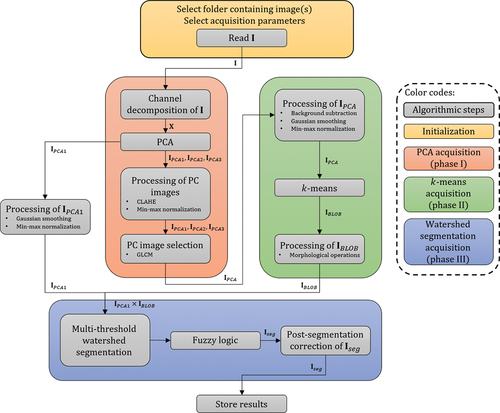
The image analysis pipeline is mainly composed of three cardinal phases (see Figure 1). Initially, the $rgb$ image, $\mathbf{I}$, is read from the selected folder, where segmentation parameters are chosen by the user in the initialisation. Phase I: the colour components of $\mathbf{I}$ are decomposed into a matrix, $\mathbf{X}$, before performing PCA on the input data. The PC images, ${\mathbf{I}}_{PCA1}$, ${\mathbf{I}}_{PCA2}$ and ${\mathbf{I}}_{PCA3}$, of the $rgb$ input sample are then processed, by means of contrast-limited adaptive histogram equalisation (CLAHE), prior to texture analysis via GLCM computation. Phase II: from the GLCM-analysis, the channel with minimum contrast is selected, ${\mathbf{I}}_{PCA}$, and supplied to the $k$-means analysis phase. The raw PC image is processed in order to augment the foreground information from the background, while restraining background information. Performing $k$-means yields a binary image of the merged colonies, ${\mathbf{I}}_{BLOB}$. Phase III: multiplying ${\mathbf{I}}_{BLOB}$ by the first PC image of $\mathbf{I}$, ${\mathbf{I}}_{PCA1}$, masks out the relevant intensity regions in preparation for watershed segmentation. Multiple intensity-thresholds are imposed on each inquired region, where respective colony features are evaluated using fuzzy logic providing a segmented binary image of ${\mathbf{I}}_{BLOB}$, ${\mathbf{I}}_{seg}$. Finally, ${\mathbf{I}}_{seg}$ is corrected post-segmentation before the conclusive results (colony count, features, etc.) are saved as .csv files.

Figure 1. Overview of the image processing pipeline showing the main steps.

2.1. Phase I: principal component analysis (PCA)

2.1.1. Image channel decomposition

We apply a decomposition method to the multivariate data composed of the $p=3$ colour channels. The idea is to identify the information about cell colonies and separate it from cell flask, shadows and noise. Originally, all of these signals are distributed across the three channels of the true colour image resulting from an optical scan of a cell flask containing stained colonies (see subsection 3.3). The proposed algorithm de-mixes the signal via a linear combination of sources using PCA. With this approach, we map colony information on a single plane by bundling the information from all colour channels (Lay et al. 2020).

Let ${\mathbf{X}}_i$ denote the observation vector in ${\mathbb{R}}^p$ comprising the red ($r$), green ($g$) and ($b$) colour components of the $i$th pixel in the $M\times N$ input image, $\mathbf{I}$. By rearranging the multichannel components, the matrix of observations, $\mathbf{X}\in {\mathbb{R}}^{p\times MN}$, is then defined to be a matrix of the form

(1) $\mathbf{X}=\left[\begin{array}{cccc}{\mathbf{X}}_1& {\mathbf{X}}_2& \cdots & {\mathbf{X}}_{MN}\end{array}\right]=\left[\begin{array}{cccc}{r}_1& r_2& \cdots & r_{MN}\\ g_1& g_2& \cdots & g_{MN}\\ b_1& b_2& \cdots & b_{MN}\end{array}\right].$(1)

The mean-deviation form matrix $\hat{\mathbf{X}}\in {\mathbb{R}}^{p\times MN}$ of $\mathbf{X}$ is introduced as ${\hat{\mathbf{X}}}_i={\mathbf{X}}_i-\mu$, for $i=1,\dots ,MN$, where $\mu$ is the sample mean of the observation matrix $\mathbf{X}$. Consequently, $\hat{\mathbf{X}}\in {\mathbb{R}}^{p\times MN}$ is introduced as

(2) $\hat{\mathbf{X}}=\left[\begin{array}{cccc}{\hat{\mathbf{X}}}_1& {\hat{\mathbf{X}}}_2& \cdots & {\hat{\mathbf{X}}}_{MN}\end{array}\right].$(2)

2.1.2. Principal component analysis (PCA)

PCA is a popular method for extracting relevant information from multivariate data, mainly focusing on dimensionality reduction (Wold et al. 1987; Abdi and Williams 2010). It aims to transform input variables linearly into PCs, sorted by their explained variance in a descending order. The main idea is that a high percentage of the total variance of the input data is covered by the first output PCs.

Technically, PCA describes the change of variable for each observation vector of $\hat{\mathbf{X}}$ by,

(3) ${\hat{\mathbf{X}}}_i=\left[\begin{array}{c}{\hat{x}}_{i1}\\ {\hat{x}}_{i2}\\ ⋮\\ {\hat{x}}_{ip}\end{array}\right]=\left[\begin{array}{cccc}{\mathbf{u}}_1& {\mathbf{u}}_2& \cdots & {\mathbf{u}}_p\end{array}\right]\left[\begin{array}{c}{\hat{y}}_{i1}\\ {\hat{y}}_{i2}\\ ⋮\\ {\hat{y}}_{ip}\end{array}\right]=\mathbf{P}{\hat{\mathbf{Y}}}_i,$(3)

where the orthogonal matrix $\mathbf{P}=\left[\begin{array}{ccc}{\mathbf{u}}_1& \cdots & {\mathbf{u}}_p\end{array}\right]\in {\mathbb{R}}^{p\times p}$ consists of the unit eigenvectors (or PCs) of the co-variance matrix of $\hat{\mathbf{X}}$, $\mathbf{C}\in {\mathbb{R}}^{p\times p}$, determined via singular value decomposition (SVD) of $\mathbf{C}$. Since $\mathbf{P}$ is an invertible matrix, a linear combination of the original variables in ${\hat{\mathbf{X}}}_i$ determines the new PC pixel values – the intensity variation of each composite $rgb$ pixel – by the variable transformation,

(4) ${\hat{y}}_{i1}={\mathbf{u}}_1^T{\hat{\mathbf{X}}}_i=u_1^{(1)}{\hat{x}}_{i1}+u_2^{(1)}{\hat{x}}_{i2}+\cdots +u_p^{(1)}{\hat{x}}_{ip},$(4)

(5) ${\hat{y}}_{i2}={\mathbf{u}}_2^T{\hat{\mathbf{X}}}_i=u_1^{(2)}{\hat{x}}_{i1}+u_2^{(2)}{\hat{x}}_{i2}+\cdots +u_p^{(2)}{\hat{x}}_{ip},$(5)

(6) ${\hat{y}}_{i3}={\mathbf{u}}_3^T{\hat{\mathbf{X}}}_i=u_1^{(3)}{\hat{x}}_{i1}+u_2^{(3)}{\hat{x}}_{i2}+\cdots +u_p^{(3)}{\hat{x}}_{ip},$(6)

where $u_1^{(1)},\dots ,u_p^{(1)}$, $u_1^{(2)},\dots ,u_p^{(2)}$ and $u_1^{(3)},\dots ,u_p^{(3)}$ are the entries in the first, second and third PC vector, ${\mathbf{u}}_1$, ${\mathbf{u}}_2$ and ${\mathbf{u}}_3$ respectively, while the new variables ${\hat{y}}_{i1}$, ${\hat{y}}_{i2}$ and ${\hat{y}}_{i3}$ represent the first, second and third PC pixel values given by ${\hat{\mathbf{Y}}}_i={\mathbf{P}}^T{\hat{\mathbf{X}}}_i$ from equation (3)(3) ${\hat{\mathbf{X}}}_i=\left[\begin{array}{c}{\hat{x}}_{i1}\\ {\hat{x}}_{i2}\\ ⋮\\ {\hat{x}}_{ip}\end{array}\right]=\left[\begin{array}{cccc}{\mathbf{u}}_1& {\mathbf{u}}_2& \cdots & {\mathbf{u}}_p\end{array}\right]\left[\begin{array}{c}{\hat{y}}_{i1}\\ {\hat{y}}_{i2}\\ ⋮\\ {\hat{y}}_{ip}\end{array}\right]=\mathbf{P}{\hat{\mathbf{Y}}}_i,$(3) . This projects an image in the first, second and third dimension of the PCA space – ${\mathbf{I}}_{PCA1}$, ${\mathbf{I}}_{PCA2}$ and ${\mathbf{I}}_{PCA3}$ respectively – reflecting the triplet colour variation of the inquired image (see Figure 2).

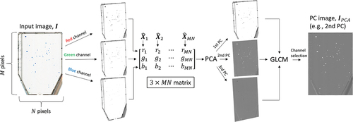
Figure 2. Schematic PCA procedure for an input image, $\mathbf{I}$. The multichannel colour image is firstly decomposed into a $3\times MN$ matrix, $\hat{\mathbf{X}}$, where each column, ${\hat{\mathbf{X}}}_i$, represents a composite, centred $rgb$ pixel. Through PCA, a linear combination of the colour channels is obtained to compose the PC images, ${\mathbf{I}}_{PCA1}$, ${\mathbf{I}}_{PCA2}$ and ${\mathbf{I}}_{PCA3}$. Dimensionality reduction is then automatically achieved by using a GLCM contrast criteria that optimally selects a single PC image for colony feature characterisation, ${\mathbf{I}}_{PCA}$.

2.1.3. Grey-level co-occurrence matrix (GLCM)

In our application, the PC images (${\mathbf{I}}_{PCA1}$, ${\mathbf{I}}_{PCA2}$, ${\mathbf{I}}_{PCA3}$) include variance information about the cell colonies, cell container, shadows and noise. Among the PC images, we assume that only one of the images offers a reliable and selective depiction of the colonies, whereas the two remaining PC images contain (variance) information representing other image contributions.

The GLCM is a statistical approach for analysing texture (Haralick et al. 1973; Haralick and Shapiro 1992). We will use image contrast, as defined from the GLCM, to identify and select the optimal PC image with respect to cell colony depiction. In a single input channel image (representing in our case one PC image), $\mathbf{J}$, the co-occurrence matrix, $\mathbf{G}\in {\mathbb{R}}^{N_g\times N_g}$, is defined as the frequency of pixel-pairs along a particular distance and direction in $\mathbf{J}$ of $N_g$ grey-levels:

(7) $g_{ij}\left(d,\theta \right)=\sum _{x=1}^N\sum _{y=1}^M\left\{\begin{array}{cc}1,& \mathrm{i}\mathrm{f}J(x,y)=i\mathrm{a}\mathrm{n}\mathrm{d}J(x+dcos\theta ,y+dsin\theta )=j\\ 0,& \mathrm{o}\mathrm{t}\mathrm{h}\mathrm{e}\mathrm{r}\mathrm{w}\mathrm{i}\mathrm{s}\mathrm{e},\end{array}\right.$(7)

(8) ${\tilde{g}}_{ij}\left(d,\theta \right)=\frac{g_{ij}\left(d,\theta \right)}{{\sum }_{i=1}^{N_g}{\sum }_{j=1}^{N_g}{g}_{ij}\left(d,\theta \right)},$(8)

where $g_{ij}\left(d,\theta \right)$ and ${\tilde{g}}_{ij}\left(d,\theta \right)$ denotes the $(i,j)$th entry in the co-occurrence matrix and normalised co-occurrence matrix, respectively. The GLCM describes the relative frequency between the pixel-pair $(x,y)$ and $(x+dcos\theta ,y+dsin\theta )$ separated by a specified displacement $d$ and angle $\theta$ – offset – with grey-level intensity $i$ and $j$, respectively, in the domain $i,j\in 1,2,\dots ,N_g$.

Next, the Haralick feature (Haralick et al. 1973) for contrast is computed from the GLCM as a statistical measure to describe colony texture characteristic and is used for PC selection

(9) $\mathrm{C}\mathrm{o}\mathrm{n}\mathrm{t}\mathrm{r}\mathrm{a}\mathrm{s}{\mathrm{t}}_{\mathbf{J}}=\sum _{i=1}^{N_g}\sum _{j=1}^{N_g}{\left|i-j\right|}^2{\tilde{g}}_{ij}(d,\theta ).$(9)

It returns a measure of the intensity contrast repetition rate for a pixel-pair across the whole image. This statistic ranges in the interval $\left[0,(N_g-{1)}^2\right]$, where it is 0 for a constant image. Therefore, low contrast entails an image that features low spatial frequencies.

The PC selection criterion involves choosing the PC image with the lowest contrast statistic. As either ${\mathbf{I}}_{PCA1}$, ${\mathbf{I}}_{PCA2}$ or ${\mathbf{I}}_{PCA3}$ expresses the colour variation of solely the colonies, the most suitable PC image is composed of pixel values that are insensitive to and suppress the presence of various high-contrast artefacts such as contaminants/residue in the suspension medium, inevitable shadow artefacts due to imaging/scanning procedures, inherent background noise emanated from the image/scan acquisition and the cell container boundary. Hence, the spatial frequency of local colour variations depicting merely the colonies is minimised in the PC image characterising the colonies relative to the remaining two PCs depicting all other elements. Hence, the PC channel with the lowest contrast results in the PC image selection describing the colonies optimally (see Figure 2):

(10) ${\mathbf{I}}_{PCA}=\underset{X\in \{{\mathbf{I}}_{PCA1},{\mathbf{I}}_{PCA2},{\mathbf{I}}_{PCA3}\}}{argmin}\mathrm{C}\mathrm{o}\mathrm{n}\mathrm{t}\mathrm{r}\mathrm{a}\mathrm{s}{\mathrm{t}}_X.$(10)

Prior to GLCM contrast estimation, each PC image is enhanced by applying CLAHE (Zuiderveld 1994) to aid the selection criterion in equation (10)(10) ${\mathbf{I}}_{PCA}=\underset{X\in \{{\mathbf{I}}_{PCA1},{\mathbf{I}}_{PCA2},{\mathbf{I}}_{PCA3}\}}{argmin}\mathrm{C}\mathrm{o}\mathrm{n}\mathrm{t}\mathrm{r}\mathrm{a}\mathrm{s}{\mathrm{t}}_X.$(10) . Through dividing an image into a grid of rectangular regions, the histogram of the contained pixels for each region is computed. The contrast of each region is locally optimised by redistributing the pixel intensity according to a transform function, where a uniform histogram equalisation distribution is used here. Then, by imposing a clip limit (or contrast factor) as a maximum on the computed histograms, over-saturation of particularly homogeneous areas (characterised by high peaks in the contextual histograms) is reduced, which prevents over-enhancement of, e.g. noise and edge-shadowing effect derived from an unlimited adaptive histogram equalisation (AHE).

2.2. Phase II: k-means clustering

To distinguish the conglomerate cell colonies characterised in ${\mathbf{I}}_{PCA}$ from background, we deploy $k$-means clustering (Lloyd 1982) on the raw ${\mathbf{I}}_{PCA}$ to produce a binary mask of the cell colonies. After subtracting the background through opening–closing by reconstruction in order to augment foreground recognition and min-max normalisation of the values to 0–1 in ${\mathbf{I}}_{PCA}$, we construct a feature matrix $\mathbf{Z}$ by aggregating the $i$th pixel value, $p_i$, with its 8-connected neighbours, $p_i^{(1)},\dots ,p_i^{(8)}$. We obtain a $9\times MN$ matrix,

(11) $\mathbf{Z}=\left[\begin{array}{cccc}{\mathbf{Z}}_1& {\mathbf{Z}}_2& \cdots & {\mathbf{Z}}_{MN}\end{array}\right]=\left[\begin{array}{cccc}{p}_1& p_2& \cdots & p_{MN}\\ p_1^{(1)}& p_2^{(1)}& \cdots & p_{MN}^{(1)}\\ ⋮& ⋮& \ddots & ⋮\\ p_1^{(8)}& p_2^{(8)}& \cdots & p_{MN}^{(8)}\end{array}\right],$(11)

where each pixel cluster ${\mathbf{Z}}_i$, $i=1,\dots ,MN$, is assigned to either background, ${\mathbf{c}}_0={\left[0,\dots ,0\right]}^T$, or foreground, ${\mathbf{c}}_1={\left[1,\dots ,1\right]}^T$, through squared Euclidean distance (ED) minimisation

(12) ${\bar{\mathbf{c}}}_i=\underset{\mathbf{c}\in \{{\mathbf{c}}_0,{\mathbf{c}}_1\}}{argmin}{∥{\mathbf{Z}}_i-\mathbf{c}∥}^2,$(12)

where ${\bar{\mathbf{c}}}_i$ denotes to the centroid of the class assigned to pixel $i$. Hence, finding the optimal distance by $k$-means ($k=2$) creates a binary mask, ${\mathbf{I}}_{BLOB}$, containing contiguous colony components denoted as Binary Large OBjects (BLOBs), $BLO{B}_1,\dots ,\dots ,BLO{B}_n$, where $n$ is the total number of BLOBs. The BLOB extraction is therefore made independent of geometrical shape as all sizes and shapes with adequate pixel intensity are masked out by $k$-means (see Figure 3).

Figure 3. Schematic $k$-means procedure for a PC image, ${\mathbf{I}}_{PCA}$. The image is used to construct a $9\times MN$ matrix, $\mathbf{Z}$, where each column,${\mathbf{Z}}_i$, represents a pixel value, $p_i$, with its 8-connected neighbours, $p_i^{(1)},\dots ,p_i^{(8)}$. Then, considering each ${\mathbf{Z}}_i$, pixel $p_i\in [0,1]$ is assigned to nearest cluster centroid ${\mathbf{c}}_0={\left[0,\dots ,0\right]}^T$ (background) or ${\mathbf{c}}_1={\left[1,\dots ,1\right]}^T$ (foreground) by minimising the ED. This results in a binary image containing appurtenant BLOBs, ${\mathbf{I}}_{BLOB}$.

2.3. Phase III: topological multi-threshold watershed segmentation

We further apply the watershed algorithm following Khan et al. (2016) and Khan et al. (2018), which we modify and expand to handle colony confluency. Here, distance transformation along multi-threshold-based watershed is consolidated with quality criteria to recursively subdivide the BLOBs of interest into distinct colonies through catchment basin and watershed line formulation (Gonzalez and Woods 2018).

The established BLOBs in ${\mathbf{I}}_{BLOB}$ are divided into individual colonies by the watershed algorithm. Watershed segmentation relies on a topographic (intensity) information across two spatial coordinates, $x$ and $y$, reflecting the colony number in each BLOB. This information is obtained from ${\mathbf{I}}_{PCA1}$ which conveys principally greyscale measure of colony intensity. Thus, by multiplying ${\mathbf{I}}_{PCA1}$ with ${\mathbf{I}}_{BLOB}$, a topographic surface is provided where the background is masked out. However, erroneous over-segmentation may result from direct application of the watershed algorithm due to noise and local irregularities in the intensity distribution. This may accordingly lead to the formation of overwhelming amounts of basin regions. Therefore, we utilise extended-minima transform to avoid the tendency to include regional minima. All regional minima are identified as connected pixels with intensities that differ more than a specified threshold, $h$, relative to neighbouring pixels, while the remaining local minima whose depths are too shallow are suppressed. The definition of the extended-minima operator for a given $h$, $\mathrm{E}-\mathrm{M}\mathrm{I}{\mathrm{N}}_h$, produces a desired binary mask of the pronounced basins,

(13) $\mathrm{E}-\mathrm{M}\mathrm{I}{\mathrm{N}}_h\left(I(x,y)\right)=\mathrm{R}-\mathrm{M}\mathrm{I}\mathrm{N}\left[R_I\left(I\left(x,y\right)+h\right)\right],$(13)

where $R_I$ denotes reconstruction by erosion of $I$ from $I+h$ to suppress all shallow minima and $\mathrm{R}-\mathrm{M}\mathrm{I}\mathrm{N}$ represents the regional minima operator of corresponding erosion.

Employing $\mathrm{E}-\mathrm{M}\mathrm{I}{\mathrm{N}}_h$ on ${\mathbf{I}}_{PCA1}$ yields varying outcomes for different thresholds, $h$. To account of this, multiple $\mathrm{E}-\mathrm{M}\mathrm{I}{\mathrm{N}}_{h_i}$, $h_i\in [h_{min},h_{max}]$, are sequentially applied on each $BLO{B}_m$, for $m=1,\dots ,n$, to create a manifold of candidate segmentation outcomes in the form of binary masks. Additionally, to withstand high cell confluency and achieve a proper segmentation, ED transform is conducted on each mask from every $h_i$. Then, the optimal transformation is selected that maximises the quality segmentation criterion, $Q$, which incorporates fuzzy logic,

(14) $h_{opt}=\underset{h_i}{argmax}Q(h_i)$(14)

(15) $Q={\mu }_1\cdot {\mu }_2\cdot {\mu }_3,$(15)

where ${\mu }_1$, ${\mu }_2$ and ${\mu }_3$ are fuzzy spline-based pi-shaped membership functions (MFs) given by

(16) ${\mu }_j\left(u\right)=\left\{\begin{array}{cc}2{\left(\frac{u-e_1^{(j)}}{e_2^{(j)}-e_1^{(j)}}\right)}^2,& e_1^{(j)}\le u\le \frac{e_1^{(j)}+e_2^{(j)}}{2}\\ 1-2{\left(\frac{u-e_2^{(j)}}{e_2^{(j)}-e_1^{(j)}}\right)}^2,& \frac{e_1^{(j)}+e_2^{(j)}}{2}\le u\le e_2^{(j)}\\ 1-2{\left(\frac{u-e_3^{(j)}}{e_4^{(j)}-e_3^{(j)}}\right)}^2,& e_3^{(j)}\le u\le \frac{e_3^{(j)}+e_4^{(j)}}{2}\\ 2{\left(\frac{u-e_4^{(j)}}{e_4^{(j)}-e_3^{(j)}}\right)}^2,& \frac{e_3^{(j)}+e_4^{(j)}}{2}\le u\le e_4^{(j)}\\ 0,& \mathrm{o}\mathrm{t}\mathrm{h}\mathrm{e}\mathrm{r}\mathrm{w}\mathrm{i}\mathrm{s}\mathrm{e},\end{array}\right.$(16)

for evaluation of colony area, circularity or expected colony count, $j=1,2,3$, respectively, represented by the variable $u$. Hence, each segmented candidate colony will have its property set $j$ for all points $u\in U$ graded according to the MF (16) such that ${\mu }_j:U\to [0,1]$. The parameters $e_1^{(j)}$, $e_2^{(j)}$, $e_3^{(j)}$ and $e_4^{(j)}$ are adjustable and correspond to the pi-shaped edges, which form the selection space (see Figure 4).

Figure 4. Schematic watershed processing pipeline for a single iterated BLOB, $BLO{B}_m$. The BLOB is extracted by the multiplication between the first PC image conversion of the input image, ${\mathbf{I}}_{PCA1}$, and the generated BLOB mask, ${\mathbf{I}}_{BLOB}$. Having the intensity representation of the conglomeration extracted, several $\mathrm{E}-\mathrm{M}\mathrm{I}\mathrm{N}$ operators and ED transforms are applied, where each transformation yields segmented colonies. The validity of each segmentation outcome is subsequently graded using fuzzy pi-shaped MF ${\mu }_j\left(u;e_1^{(j)},e_2^{(j)},e_3^{(j)},e_4^{(j)}\right)$ for a fuzzy set $j$ representing colony area, circularity and expected count.

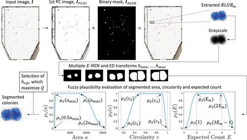
For ${\mu }_1$, the corners of the area distribution are

$\left(e_1^{(1)},e_2^{(1)},e_3^{(1)},e_4^{(1)}\right)=\left(0.5a_{min},a_{min},max\left(2a_{min},a_{max}\right),2a_{max}\right),$

where $a_{min}$ and $a_{max}$ are minimum and maximum user specified colony sizes, respectively. For ${\mu }_2$, the circularity parameters are flexible $\left(e_1^{(2)},e_2^{(2)},e_3^{(2)},e_4^{(2)}\right)\left(c_1,c_2,c_3,c_4\right)$, where $0\le c_1<c_2<c_3<c_4\le 1$ with circularity value 1 for a perfect circle. For the expected count distribution ${\mu }_3$, the function edges are defined as $\left(e_1^{(3)},e_2^{(3)},e_3^{(3)},e_4^{(3)}\right)=\left(1,E_m,2E_m,3E_m-1\right)$, where $E_m=⌈\frac{a_m}{\tilde{a}}⌉$, $a_m$ is the area of $BLO{B}_m$ and $\tilde{a}$ is the median area of $BLO{B}_1,\dots ,BLO{B}_n$. Thus, the multi-feature fuzzy logic presented is utilised to assess the geometrical shapes of subdivided colonies within an iterated $BLO{B}_m$ after each successive watershed segmentation. This is performed in order to objectively select the segmented outcome that attains colonies of coherent geometrical characteristics. Ultimately, the segmentation procedure yields an appropriate binary image representing the final feature-endorsed colonies, ${\mathbf{I}}_{seg}$.

3. Experimental set-up and data acquisition

3.1. Parameter selection

The images are loaded in the ACC algorithm and the parameters are manually tuned as listed in Table 1 for each data set. During the PCA acquisition (phase I), the PC images are firstly processed using CLAHE in preparation for the GLCM contrast selection criterion. The contrast enhancement is performed by partitioning each image into $16\times 16$ regions with a clip limit factor of $0.008$. For the computation of the co-occurrence matrix, $\mathbf{G}$, in equation (8)(8) ${\tilde{g}}_{ij}\left(d,\theta \right)=\frac{g_{ij}\left(d,\theta \right)}{{\sum }_{i=1}^{N_g}{\sum }_{j=1}^{N_g}{g}_{ij}\left(d,\theta \right)},$(8) the spatial dependence between neighbouring pixels was evaluated at $N_g=64$ grey-levels. Further, the GLCM is highly dependent on the parameters $d$ and $\theta$. Thus, applying equation (8)(8) ${\tilde{g}}_{ij}\left(d,\theta \right)=\frac{g_{ij}\left(d,\theta \right)}{{\sum }_{i=1}^{N_g}{\sum }_{j=1}^{N_g}{g}_{ij}\left(d,\theta \right)},$(8) , several matrices were obtained for each change in direction $\theta$. This was defined by four different offset vectors; $[0,d]$ ($\theta =0^{\circ }$), $[-d,d]$ ($\theta ={45}^{\circ }$), $[-d,0]$ ($\theta ={90}^{\circ }$), $[-d,-d]$ ($\theta ={135}^{\circ }$), where the displacement $d=1$ (in pixels) is set to examine merely adjacent pixels in $\mathbf{J}$ (the PC images). The co-occurrence matrix and thereby the contrast statistic was readily computed for each offset and then averaged. The choice of $d$ is justified as a pixel is more likely to be correlated to closely located pixels than those further away.

Table 1. Parameter selection in the automated colony counting (ACC) method for image segmentation of the different clonogenic species. The Gaussian smoothing filter size, $s_x\times s_y$, specified as a 2-element vector of positive numbers in terms of the standard deviation, $\sigma$, of the Gaussian distribution, is applied on ${\mathbf{I}}_{PCA}$ and ${\mathbf{I}}_{PCA1}$. The radius of the disk-shaped structuring element in the morphological opening-closing by reconstruction, $r_{obrcbr}$, is given in pixels. Minimum and maximum user specified colony areas, $a_{min}$ and $a_{max}$ respectively, are given in pixels.

Data Set	Specie	Acquisition Parameters
		$s_x\times s_y$	$s_x\times s_y$	$r_{obrcbr}$	$(a_{min},a_{max})$
		(${\mathbf{I}}_{PCA}$)	(${\mathbf{I}}_{PCA1}$)	(pixels)	(pixels)
1	T-47D	$2\sigma \times 2\sigma$	$4\sigma \times 4\sigma$	$40$	$(40,8000)$
2	E. coli	$3\sigma \times 3\sigma$	$10\sigma \times 10\sigma$	$90$	$(1000,35000)$
	Klebs. pn.	$3\sigma \times 3\sigma$	$6\sigma \times 6\sigma$	$65$	$(800,20000)$
	Pseud. ae.	$3\sigma \times 3\sigma$	$8\sigma \times 8\sigma$	$80$	$(2500,20000)$
	Staph. au.	$3\sigma \times 3\sigma$	$6\sigma \times 6\sigma$	$30$	$(500,5000)$

For the $k$-means acquisition (phase II), the processing stage of ${\mathbf{I}}_{PCA}$ included morphological opening–closing by reconstruction using a disk-shaped structuring element with a radius of $r_{obrcbr}$ (in pixels), before smoothing using a filter with a 2D Gaussian kernel of size $s_x\times s_y$ (see Table 1). These operations were used for background suppression and to smooth the varying spatial image intensity for outliers, respectively. Here, $r_{obrcbr}$ should conform with areas size of the BLOBs as it should be exceedingly greater, whereas $s_x\times s_y$ should reduce evident noise over smaller spatial regions. In the processing step of ${\mathbf{I}}_{BLOBs}$, various morphological operations were applied on the binary mask such as dilation and flood-filling of holes.

${\mathbf{I}}_{PCA1}$ was also processed prior to the watershed segmentation: 2D Gaussian filtering (to avoid over-segmentation of the BLOBs) was employed, where the enhanced image was min-max normalised (see Table 1). The Gaussian smoothing on ${\mathbf{I}}_{PCA1}$ is set to directly affect the forthcoming segmentation of the extracted BLOBs as the filtering is performed on regions in ${\mathbf{I}}_{PCA1}$ masked out by ${\mathbf{I}}_{BLOBs}$. Depending on the image dpi, area size of the actual colonies and colony confluency, the standard deviation of the Gaussian blur of the BLOB greyscale intensities should be chosen accordingly.

During the watershed segmentation (phase III), each masked $BLO{B}_m$ having an area $a_m>a_{thresh}=0.6\tilde{a}$ and circularity $c_m<0.6$ was further separated through the multi-threshold segmentation. These condition limits for segmentation were kept fixed. Enforcing this, we chose $h_i\in [h_{min},h_{max}]=[0.15,0.37]$ with incremental steps ${\mathrm{\Delta }}_h=0.01$ as a search space for all data sets. The size of this watershed search space has a pronounced influence on the runtime; even though a smaller range and/or larger ${\mathrm{\Delta }}_h$ would yield a shorter computation time, doing so may not ensure optimal segmentation results. Thus, a high colony density necessitates a large search span by lowering the $h_{min}$ value to eventuate a finer segmentation of BLOBs, while choosing a very large $h_{max}$ value may not be cost-effective. The pi-shaped MF parameters for the area and circularity distributions were fixed to $\left(0.5a_{min},a_{min},a_{max},2a_{max}\right)$ and $\left(c_1,c_2,c_3,c_4\right)=\left(0.15,0.5,0.9,1\right)$, respectively, where $a_{min}$ and $a_{max}$ (in pixels) are provided by the user (see Table 1). The edges for the expected colony count within each iterated $BLO{B}_m$, $\left(1,E_m,2E_m,3E_m-1\right)$, are adaptively computed throughout the segmentation process. Subsequent segmented colonies were recursively divided until the criterion $a_m\le a_{thresh}$ was met.

3.2. Cell culture and manual counting

Human breast ductal cell carcinoma cells of the T-47D line were cultured in RPMI medium (Lonza), supplemented with 10% FBS (Biochrom), 1% penicillin/streptomycin (Lonza) and 200 units per litre insulin (Gibco), at 37°C in air with 5% CO₂. The cells were kept in exponential growth by reculturing twice per week with one additional medium change per week. The seeded number of cells was low which consequently formed sparsely populated colonies in each T25 culture flask (25 cm² cell culture area; Nunclon, Denmark). For more information on the cell culture and colony formation assay used in the current work, see e.g. Edin et al. (2012).

To validate the quality of the presented ACC segmentation algorithm, we compared the ACC number to the number produced by the recently published method AutoCellSeg (Khan et al. 2018) (both proprietary and open-source data), as well as to the manual colony counting (MCC) facilitated by three trained human observers (only proprietary data). Here the observers were independent meaning that no subject could know the results of any other before counting. Additionally, an extra independent observer established a GT by manual counting during a microscopic analysis of the culture dishes for comparison (proprietary data).

3.3. Data description

The ACC algorithm was applied to the images of the cell culture flasks containing fixed and stained cell colonies. We conducted experiments on both proprietary and open-source data.

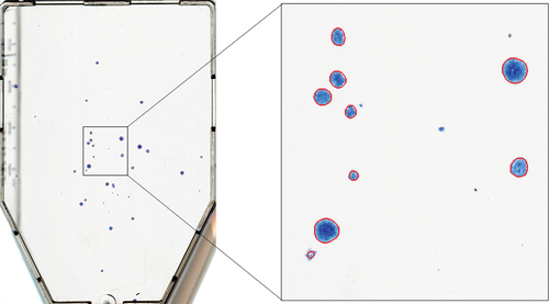
Proprietary data (data set 1) were obtained from a flatbed laser scanner (Epson Perfection V850 Pro), providing $rgb$ images with a resolution of 2125 $\times$ 2985, 1200 dots per inch (dpi), 21.17µm/pixel spatial resolution and 48-bit depth. No prior filtering nor adjustments were performed on the captured images during scanning with the scanner software (EPSON Scan v3.9.3.3). Data set 1, including respective MCC and GT data, is publicly available in Zenodo’s repository (Arous et al. 2021). An example of cell colony image is provided in Figure 5. The cell flask contains cell colonies, as well as background structures (e.g. shadows) and outer contours of the T25 cell flask. The segmentation suggested by the ACC is delineated in red. The full data set consists of 16 cell culture flasks used for a colony formation assay of the T-47D (breast) cancer cell line.

Figure 5. Example image from data set 1. The segmentation suggested by the automated colony counting (ACC) algorithm is outlined in red.

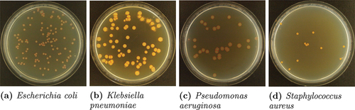
Open-source images (data set 2) of $rgb$ colour representation, 4032 $\times$ 3024 resolution, 314 dpi, 80.89 $\mu$ m/pixel spatial resolution and 24-bit depth, with accompanying GT delineations, were obtained from the publicly available AutoCellSeg’s GitHub repository (https://github.com/AngeloTorelli/AutoCellSeg/tree/master/DATA/Benchmark). The data set contained 12 images of four bacterial species (3 images each), including Escherichia coli (E. coli), Klebsiella pneumoniae (Klebs. pn.), Pseudomonas aeruginosa (Pseud. ae.) and Staphylococcus aureus (Staph. au.) cultured in Petri dishes. The GT colony delineations were produced by the authors Torelli et al. using Adobe Photoshop before being converted into binary masks. Delineations obtained for this data set using the ACC algorithm are shown in Figure 6.

Figure 6. Example images from data set 2. The segmentation suggested by the automated colony counting (ACC) algorithm is outlined in red.

3.4. Hardware

The segmentation using the ACC procedure was implemented in MATLAB (MathWork, Natick, MA, USA) and executed on an Intel Core i7-8565 U CPU @ 1.80 GHz with 16 GB RAM. The average runtime of the proposed algorithm was 114 seconds per image, which is adequate when considering the software as a fully automated batch throughput solution for large data sets. However, runtime optimisation and parallelisation are not in the scope of this work and will be considered in future projects. The AutoCellSeg results were obtained by installing and utilising the freely available AutoCellSeg software (https://github.com/AngeloTorelli/AutoCellSeg), which is based on the open-source implementation by Torelli et al., and run on a partially automated mode via the GUI with similar processing parameters as in our own pipeline.

3.5. Statistical analysis

In addition to cell colony counts, we investigated the spatial information associated with the detected cell colonies in the images. Hence, Table 2 further provides binary classification metrics for both ACC and AutoCellSeg using a region-wise definition of the confusion matrix. Given the segmentation of ACC or AutoCellSeg, respectively, as well as one centralised coordinate point per colony representing the GT (GT mark), we considered a colony as detected if at least one GT mark was within the delineated area. Such regions were denoted as true positives ($TP$). We denoted a cell colony as false positive ($FP$) if the delineated region did not contain any GT mark. Finally, false negative ($FN$) regions were obtained from those GT marks which were either located outside the delineated areas (not detected by the algorithm) or in a delineated region together with other GT marks (merged with other colonies by the algorithm). The $F_1$ score was chosen as a binary classification metric to measure the spatial accuracy of the detected colonies made by the observers and the ACC. Here the $F_1$ score is the harmonic mean between the precision and recall:

(17) $F_1=\frac{2}{\mathrm{p}\mathrm{r}\mathrm{e}\mathrm{c}\mathrm{i}\mathrm{s}\mathrm{i}\mathrm{o}{\mathrm{n}}^{-1}+\mathrm{r}\mathrm{e}\mathrm{c}\mathrm{a}\mathrm{l}{\mathrm{l}}^{-1}}=\frac{2}{{\left(\frac{TP}{TP+FP}\right)}^{-1}+{\left(\frac{TP}{TP+FN}\right)}^{-1}},$(17)

Table 2. Statistical results for 16 T-47D cell flask images (data set 1) presented as mean $\pm$ standard deviation [min, max], obtained from our automated colony counting (ACC) procedure, the AutoCellSeg method, as well as manual colony counting (MCC), when compared to the ground truth (GT).

	ACC	AutoCellSeg
Precision	$0.96\pm 0.024[0.91,1.00]$	$0.86\pm 0.051[0.76,0.93]$
Recall	$0.85\pm 0.072[0.68,0.94]$	$0.77\pm 0.097[0.61,0.93]$
$F_1$	$0.90\pm 0.049[0.78,0.96]$	$0.81\pm 0.064[0.71,0.93]$
APE	$11.5\pm 7.2[1.9,27.5]\mathrm{\%}$	$11.3\pm 10.3[0,34.4]\mathrm{\%}$

Estimates for colony count, precision, recall, F₁ score and absolute percentage error (APE) produced by each method are compared.

where the precision is a measure of exactness (the ratio of $TP$ cases to the total predicted positive cases, $TP+FP$), while recall is a measure of completeness (the ratio of $TP$ cases to the total actual positives cases, $TP+FN$).

4. Results

4.1. Data set 1

Figure 7 shows an overview on the results from ACC, AutoCellSeg and MCC, as well as their respective values compared to the GT on data set 1. Even though both MCC and GT were obtained from manual counting, the former was based on manual counting on the same images that were presented to the algorithm, whereas the GT is more reliable due to the in-depth information from the microscopy. For each image, the average MCC is shown along with its mean absolute deviation between the observers. As shown in Figure 7, both ACC and AutoCellSeg have tendencies to underestimate the number of colonies. Corresponding statistical measures of colony count, precision, recall, $F_1$ score and absolute percentage error (APE) are listed in Table 2. From Table 2, the values of precision, recall and $F_1$ score of the proposed system are greater than the AutoCellSeg method, while the APE where comparable between the two methods; 11.5% and 11.3% for ACC and AutoCellSeg, respectively. However, MCC resulted in 3.7% APE.

Figure 7. Relationship between the counts for the three methods – automating colony counting (ACC) (circle), AutoCellSeg (square), manual colony counting (MCC) (triangle) – and ground truth (GT) counts for data set 1 (T-47D colonies). Mean MCC is shown along with its standard deviation between the 3 observers. The stippled line is the identity line.

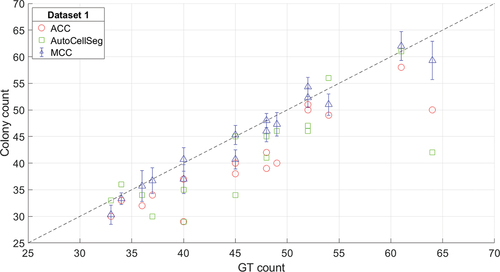
The counts obtained from all methods achieve similar results and do not show a clear winner: our proposed ACC method produced a root-mean-square error (RMSE) of 14% with a tendency to underestimate the GT count. AutoCellSeg showed similar characteristics with an RMSE of 17%. Although the MCC had a similar RMSE (ACC errors are within the error bounds associated with MCC), the manual observers slightly overestimated the colony number: in all except for three images, the mean MCC was higher than the GT count (see Figure 7).

With regard to spatial information, ACC obtained superior $F_1$ scores compared to AutoCellSeg, although the absolute ranges for both procedures were on a very high level ($F_1$ score mostly $>90$%). This indicates that ACC can outperform the current state-of-the method. Analysing the metrics in detail revealed that in most cases, both precision and recall could be improved by ACC. In few cases, we observe that ACC obtains a higher $F_1$ score, although the error with respect to absolute colony counts is higher compared to AutoCellSeg. This anomaly might be caused by a mutual compensation of different error types in AutoCellSeg, such as dividing one cell colony into multiple regions and neglecting others at the same time. This will decrease the $F_1$ score, but remain undisclosed when comparing overall colony counts.

4.2. Data set 2

In addition to the results obtained from the proprietary T-47D cell data set, we used both algorithms, ACC and AutoCellSeg, on publicly available open-source data sets. The data sets differ from data set 1 in colouring, shape of the cell dish, size of the investigated cell colonies, image resolution and background. Evaluation is made in the same way as for data set 1, except for that no manual counting from different observers was available for evaluation.

From Figure 8, ACC demonstrated a slightly better performance compared to AutoCellSeg. This conforms with the overall statistical results in Table 3, where the experiment conducted on data set 2 demonstrates that ACC is able to outperform AutoCellSeg with respect to precision, recall, $F_1$ score and APE. In fact, ACC is superior to AutoCellSeg in 9 out of 12 cases with respect to $F_1$ scores and performs equally well in 2 cases, whereas AutoCellSeg scored higher on only 1 case. Indirectly, the presented results can be compared to experiments from (Khan et al. 2018) on the same data sets, where other recent methods are evaluated. Unlike for data set 1, the single images in this experiment show more variability, hence the high-quality results underline the flexibility of the presented algorithm.

Figure 8. Relationship between the counts for the two methods – automating colony counting (ACC) (circle), AutoCellSeg (square) – and ground truth (GT) counts for data set 2 (bacterial colonies). Data for Escherichia coli (E. coli) (red), Klebsiella pneumoniae (Klebs. pn.) (green), Pseudomonas aeruginosa (Pseud. ae.) (blue) and Staphylococcus aureus (Staph. au.) (cyan) are presented. The stippled line is the identity line.

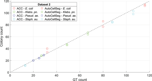
Table 3. Statistical results for 12 bacterial colony Petri dish images (data set 2).

Specie		ACC	AutoCellSeg
E. coli	Precision	$0.97\pm 0.025[0.94,0.99]$	$0.89\pm 0.090[0.80,0.98]$
	Recall	$0.97\pm 0.031[0.94,1.00]$	$0.98\pm 0.021[0.96,1.00]$
	$F_1$	$0.97\pm 0.0058[0.96,0.97]$	$0.93\pm 0.040[0.89,0.97]$
	APE	$4.5\pm 1.5[3.5,6.3]\mathrm{\%}$	$11.4\pm 12.1[1.7,25.0]\mathrm{\%}$
Klebs. pn.	Precision	$0.98\pm 0.021[0.96,1.00]$	$0.97\pm 0.031[0.94,1.00]$
	Recall	$0.98\pm 0.032[0.94,1.00]$	$0.96\pm 0.051[0.90,1.00]$
	$F_1$	$0.98\pm 0.010[0.97,0.99]$	$0.96\pm 0.035[0.92,0.98]$
	APE	$3.3\pm 3.1[0,6.1]\mathrm{\%}$	$4.1\pm 0.4[3.7037,4.5]\mathrm{\%}$
Pseud. ae.	Precision	$0.99\pm 0.023[0.96,1.00]$	$0.97\pm 0.025[0.95,1.00]$
	Recall	$0.97\pm 0.046[0.92,1.00]$	$0.96\pm 0.010[0.95,0.97]$
	$F_1$	$0.98\pm 0.035[0.94,1.00]$	$0.97\pm 0.015[0.95,0.98]$
	APE	$1.3\pm 2.3[0,4.0]\mathrm{\%}$	$1.3\pm 2.3[0,4.0]\mathrm{\%}$
Staph. au.	Precision	$0.99\pm 0.015[0.97,1.00]$	$0.98\pm 0.025[0.95,1.00]$
	Recall	$0.94\pm 0.015[0.92,0.95]$	$0.89\pm 0.040[0.85,0.93]$
	$F_1$	$0.96\pm 0.0058[0.96,0.97]$	$0.93\pm 0.021[0.91,0.95]$
	APE	$4.6\pm 2.7[2.8,7.7]\mathrm{\%}$	$9.2\pm 5.6[4.6,15.4]\mathrm{\%}$

The results are presented as mean ± standard deviation [min, max] (3 images per specie), obtained from automated colony counting (ACC) via the presented procedure, as well as the AutoCellSeg method, when compared to the ground truth (GT). Estimates for colony count, precision, recall, F₁ score and absolute percentage error (APE) produced by each method are compared.

5. Discussion

A clear benefit of the proposed ACC algorithm is the saving of resources in terms of time and manual effort. Remarkably, the algorithm matches manual observation techniques not only in terms of speed but also delivers robust and objective results.

Our experiments demonstrated that the proposed algorithm is capable of solving the automated cell counting problem and serves as a valid alternative to manual procedures with a competitive quality. Herein, the PC image containing the colour variability of the colonies offers a reliable and selective depiction of the colonies when compared to the traditional greyscale image, ${\mathbf{I}}_{grey}$, of $\mathbf{I}$. Without PCA, feature extraction from ${\mathbf{I}}_{grey}$ is liable to include and segment falsely detected objects with similar greyscale intensities as colonies. Also, the results are superior to those obtained from the AutoCellSeg state-of-the-art method and in the range of human inter-observer variance. Thus, further refinement is hardly possible unless more accurate reference data are available. In particular, the flexibility of our presented ACC algorithm, taking different cell dish geometries, background, image resolution and colouring into account, proved its high value.

We discovered a small bias between the human observers and the automated counts, particularly on data set 1. In this case, the algorithm tends to provide lower estimates. A manual evaluation showed that particularly small and sparsely populated cell regions with low contrast to the background were neglected by the automated algorithm in specific cases, but identified as colonies by human observers. Such errors can be reduced by parameter tuning, particularly those related to watershed segmentation. However, the fact that the results from different human observers are not always consistent (in particular when judging such small regions) shows the challenges of the task. Following the definition of cell colonies as conglomerations of more than typically 50 cells, this threshold can solely be verified by microscopy. Enhanced parameter tuning procedures to fit different problem set-ups will be investigated in the future work when reliable GT information is available for a larger amount of data.

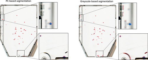
In order to substantiate the significance of the PCA (phase I), a comparison in colony segmentation performance delivered by ACC was done when feeding ${\mathbf{I}}_{grey}$ rather than ${\mathbf{I}}_{PCA}$ into the $k$-means procedure (phase II). A demonstration is shown in Figure 9. Estimates of precision, recall and $F_1$ score were $0.71\pm 0.085[0.59,0.89]$, $0.92\pm 0.043[0.82,1.00]$ and $0.80\pm 0.052[0.71,0.92]$, respectively. Thus, the precision decreases significantly, i.e. it delivers many $FP$ s as shadow and cell container segments get thresholded and included further downstream in the pipeline.

Figure 9. Demonstration of colony segmentation performance on an image from data set 1 when PCA (left) versus conventional greycale conversion (right) of the input image $\mathbf{I}$ is used in the pipeline. The segmentation suggested by the automated colony counting (ACC) algorithm is outlined in red.

A similar automated colony segmentation procedure has been proposed, using an ad-hoc image capture system for Petri dishes (Chiang et al. 2015). The image processing pipeline employed PCA to convert acquired colour images into intensity, Otsu’s method (Otsu 1979) to extract E. coli K12 bacterial colonies and distance transform along with watershed to separate clustered colonies. Although the mean values of precision, recall and $F_1$ score are all reported to be 0.96 with 3.37% mean absolute percentage error, the colony counting results rely solely on images captured in the built hardware apparatus that provides sufficient back lighting. Therein, it is unclear as to which PC channel is exploited. Also, the segmentation was only tested on a single bacteria colony strain, leaving features of colonies with different colours and opacity uninvestigated. Contrarily, our proposed algorithm has been proved on images of various colony strains with different characteristics (size, shape, contrast, colouration) acquired by a general-purpose flatbed scanner.

A recent alternative solution for cell colony detection employs the assumption that there is a strict proportionality between area of the dish covered by the colonies and the number of colonies, rather than quantifying the exact count of colonies directly (Militello et al. 2020). Within this area-based approach, multi-feature fuzzy clustering is leveraged by considering local entropy and standard deviation in the input colour images, where colony formation was chosen as the main quantity of interest. Albeit yielding colony counts that correlate well with manual measurements on four human cell lines, the method does however not provide further segmentation of the extracted merged areas from the background.

In addition, identification of the centroid coordinates of each colony listed together with information about respective colony ID, area, circularity and mean/standard deviation of intensity (colour, greyscale and PCs) distribution as well as colony count are saved for further analysis upon completion of our segmentation procedure. Moreover, a binary mask containing fully filled areas representing the segmented colonies is also saved for each image. Thus, the culminated output from the algorithm could open for new applications with colony formation assays beyond regular colony counting. This is useful for users who, for instance, wish to evaluate the colony size of a distinct cell population with respect to treatment efficacy of, e.g. irradiation or a drug.

Compared to other contemporary problems in digital image processing and computer vision, the available amount of training and test data is very limited and the GT is not completely unbiased. Hence, complex models such as CNNs are hardly applicable. Instead, the presented algorithm is unsupervised and overcomes the limitations imposed from the training data by building on well-established and easy-to-train components. An extension with other architectures will be evaluated when more training data are available in the future. Moreover, translating the proposed algorithm into other languages such as Python, R, etc. is also valuable as it allows for more flexibility to extend the program in various programming languages with their complementary packages or modules.

6. Conclusion

We presented a novel algorithm to segment cell colonies on images of cell dishes from colony formation experiments. Our ACC procedure is based upon a tailored pipeline with three major components: PCA bundles the information content from the $rgb$ colour channels, $k$-means clustering identifies conglomerate areas of cell colonies and a fuzzy statistics modification of the watershed algorithm splits them into separate cell colonies.

Our experiments were conducted on a breast cancer cell line as well as publicly available images from other cell types. In our analyses, the method was evaluated against both a recent state-of-the-art method and manual counting by human experts. The experiments demonstrated that the proposed algorithm is able to beat the benchmark, as well as it meets the expectations by obtaining results of similar quality as the manual observers.

Acknowledgments

We would like to thank Julia Marzioch, Olga Zlygosteva and Magnus Børsting from the Department of Physics at the University of Oslo for conducting the manual counting of the cell colonies.

Disclosure statement

No potential conflict of interest was reported by the author(s).

Additional information

Funding

This work was supported by the South-Eastern Norway Regional Health Authority under Helse Sør-Øst RHF Project ID 2019050 and the Norwegian Cancer Society under Grant ID 182672.

Notes on contributors

Delmon Arous

Delmon Arous is a PhD fellow in the Department of Physics at the University of Oslo, section of Biophysics and Medical Physics, where he received a Master’s degree in physics in the same section. His work focuses specifically on Monte Carlo simulations of radiation transport, dosimetry and quantitative image analysis for facilitating, among other, in vivo studies of radiation effects in the head and neck of mice.

Stefan Schrunner

Stefan Schrunner received his PhD degree in computer science from Graz University of Technology, Austria, in 2019. He is currently a post-doctoral fellow in data science at the Norwegian University of Life Sciences. His research interests are machine learning and applied statistics, including time series analysis, image processing, pattern recognition and Bayesian models.

Ingunn Hanson

Ingunn Hanson received her MSc degree in Nanotechnology from the Norwegian University of Science and Technology in 2018. She is currently working on her PhD project in Radiobiology at the Section of Medical Physics and Biophysics, University of Oslo. Her work focuses on chemical radioprotection and radio-mitigation on the cellular and organism-wide level.

Nina Frederike Jeppesen Edin

Nina Frederike Jeppesen Edin has a PhD in physics. She works as associate professor and head of Section for Biophysics and Medical Physics at University of Oslo.

Eirik Malinen

Eirik Malinen holds a PhD in biophysics and is professor at the Department of Physics, University of Oslo, Norway. He is engaged in radiation physics research as well as preclinical and clinical investigations utilising ionising radiation.

References

- Abdi H, Williams LJ. 2010. Principal component analysis. Wiley Interdiscip Rev Comput Stat. 2(4):433–459. doi:10.1002/wics.101.
- Akram SU, Kannala J, Eklund L, and Heikkilä J. 2016. Cell segmentation proposal network for microscopy image analysis. In: Deep learning and data labeling for medical applications. New York (NY): Springer; p. 21–29.
- Albaradei SA, Napolitano F, Uludag M, Thafar M, Napolitano S, Essack M, Bajic VB, Gao X. 2020. Automated counting of colony forming units using deep transfer learning from a model for congested scenes analysis. IEEE Access. 8:164340–164346. doi:10.1109/ACCESS.2020.3021656.
- Arous D, Schrunner S, Hanson I, FJ Edin N, and Malinen E. 2021. Cell colony image segmentation dataset 1 for T-47D breast cancer cells. doi:10.5281/zenodo.4593510.
- Bewes J, Suchowerska N, McKenzie D. 2008. Automated cell colony counting and analysis using the circular Hough image transform algorithm (chita). Phys Med Biol. 53(21):5991. doi:10.1088/0031-9155/53/21/007.
- Breiman L. 2001. Random forests. Mach Learn. 45(1):5–32. doi:10.1023/A:1010933404324.
- Cai Z, Chattopadhyay N, Liu WJ, Chan C, Pignol JP, Reilly RM. 2011. Optimized digital counting colonies of clonogenic assays using ImageJ software and customized macros: comparison with manual counting. Int J Radiat Biol. 87(11):1135–1146. doi:10.3109/09553002.2011.622033.
- Carpenter AE, Jones TR, Lamprecht MR, Clarke C, Kang IH, Friman O, Guertin DA, Chang JH, Lindquist RA, Moffat J, et al. 2006. Cellprofiler: image analysis software for identifying and quantifying cell phenotypes. Genome Biol. 7(10):R100. doi:10.1186/gb-2006-7-10-r100.
- Chiang PJ, Tseng MJ, He ZS, Li CH. 2015. Automated counting of bacterial colonies by image analysis. J Microbiol Methods. 108:74–82. doi:10.1016/j.mimet.2014.11.009.
- Choudhry P. 2016. High-throughput method for automated colony and cell counting by digital image analysis based on edge detection. PloS one. 11(2):e0148469. doi:10.1371/journal.pone.0148469.
- Clarke ML, Burton RL, Hill AN, Litorja M, Nahm MH, Hwang J. 2010. Low-cost, high-throughput, automated counting of bacterial colonies. Cytometry Part A. 77A(8):790–797. doi:10.1002/cyto.a.20864.
- Edin NJ, Olsen DR, Sandvik JA, Malinen E, Pettersen EO. 2012. Low dose hyper-radiosensitivity is eliminated during exposure to cycling hypoxia but returns after reoxygenation. Int J Radiat Biol. 88(4):311–319. doi:10.3109/09553002.2012.646046.
- Falk T, Mai D, Bensch R, Çiçek Ö, Abdulkadir A, Marrakchi Y, Böhm A, Deubner J, Jäckel Z, Seiwald K, et al. 2019. U-net: deep learning for cell counting, detection, and morphometry. Nat Methods. 16(1):67–70. doi:10.1038/s41592-018-0261-2.
- Ferrari A, Lombardi S, Signoroni A. 2017. Bacterial colony counting with convolutional neural networks in digital microbiology imaging. Pattern Recognit. 61:629–640. doi:10.1016/j.patcog.2016.07.016.
- Franken NA, Rodermond HM, Stap J, Haveman J, Van Bree C. 2006. Clonogenic assay of cells in vitro. Nat Protoc. 1(5):2315. doi:10.1038/nprot.2006.339.
- Geissmann Q. 2013. Opencfu, a new free and open-source software to count cell colonies and other circular objects. PloS one. 8(2):e54072. doi:10.1371/journal.pone.0054072.
- Gonzalez RC, Woods RE. 2018. Digital image processing. New York (NY): Pearson.
- Haralick RM, Shanmugam K, Dinstein IH. 1973. Textural features for image classification. IEEE Trans Syst Man Cybern. 6(6):610–621. doi:10.1109/TSMC.1973.4309314.
- Haralick RM, and Shapiro LG. 1992. Computer and robot vision. Vol. 1. Boston (MA): Addison-wesley Reading.
- Junkin M, Tay S. 2014. Microfluidic single-cell analysis for systems immunology. Lab Chip. 14(7):1246–1260. doi:10.1039/c3lc51182k.
- Khan AUM, Mikut R, Reischl M. 2016. A new feedback-based method for parameter adaptation in image processing routines. PloS one. 11(10):e0165180. doi:10.1371/journal.pone.0165180.
- Khan A.u.M, Torelli A, and Wolf I, et al. 2018. AutoCellSeg: robust automatic colony forming unit (CFU)/cell analysis using adaptive image segmentation and easy-to-use post-editing techniques. Sci Rep. 8(1):1–10. doi:10.1038/s41598-017-17765-5.
- Krastev DB, Slabicki M, Paszkowski-Rogacz M, Hubner NC, Junqueira M, Shevchenko A, Mann M, Neugebauer KM, Buchholz F. 2011. A systematic RNAi synthetic interaction screen reveals a link between p53 and snornp assembly. Nat Cell Biol. 13(7):809–818. doi:10.1038/ncb2264.
- Lay DC, Lay SR, McDonald J. 2020. Linear algebra and its applications. Boston (MA): Pearson.
- Lloyd S. 1982. Least squares quantization in pcm. IEEE Trans Inf Theory. 28(2):129–137. doi:10.1109/TIT.1982.1056489.
- Mansberg H. 1957. Automatic particle and bacterial colony counter. Science. 126(3278):823–827. doi:10.1126/science.126.3278.823.
- Militello C, Rundo L, Conti V, Minafra L, Cammarata FP, Mauri G, Gilardi MC, Porcino N. 2017. Area-based cell colony surviving fraction evaluation: a novel fully automatic approach using general-purpose acquisition hardware. Comput Biol Med. 89:454–465. doi:10.1016/j.compbiomed.2017.08.005.
- Militello C, Rundo L, Minafra L, Cammarata FP, Calvaruso M, Conti V, Russo G. 2020. Mf2c3: multi-feature fuzzy clustering to enhance cell colony detection in automated clonogenic assay evaluation. Symmetry. 12(5):773. doi:10.3390/sym12050773.
- Moiseenko V, Duzenli C, Durand RE. 2007. In vitro study of cell survival following dynamic MLC intensity-modulated radiation therapy dose delivery. Med Phys. 34(4):1514–1520. doi:10.1118/1.2712044.
- Otsu N. 1979. A threshold selection method from gray-level histograms. IEEE Trans Syst Man Cybern. 9(1):62–66. doi:10.1109/TSMC.1979.4310076.
- Ronneberger O, Fischer P, and Brox T 2015. U-net: convolutional networks for biomedical image segmentation. In: International Conference on Medical image computing and computer-assisted intervention, 2015 Munich, Germany. Springer. p. 234–241 doi:10.1007/978-3-319-24574-4_28.
- Sadanandan SK, Ranefall P, Le Guyader S, Wählby C. 2017. Automated training of deep convolutional neural networks for cell segmentation. Sci Rep. 7(1):1–7. doi:10.1038/s41598-017-07599-6.
- Schindelin J, Arganda-Carreras I, Frise E, Kaynig V, Longair M, Pietzsch T, Preibisch S, Rueden C, Saalfeld S, Schmid B, et al. 2012. Fiji: an open-source platform for biological-image analysis. Nat Methods. 9(7):676–682. doi:10.1038/nmeth.2019.
- Sergioli G, Militello C, Rundo L, Minafra L, Torrisi F, Russo G, Chow KL, Giuntini R. 2021. A quantum-inspired classifier for clonogenic assay evaluations. Sci Rep. 11(1):1–10. doi:10.1038/s41598-021-82085-8.
- Siragusa M, Dall’Olio S, Fredericia PM, Jensen M, Groesser T. 2018. Cell colony counter called coconut. PloS one. 13(11):e0205823. doi:10.1371/journal.pone.0205823.
- Sommer C, Straehle C, Koethe U, and Hamprecht FA 2011. Ilastik: interactive learning and segmentation toolkit. In: 2011 IEEE international symposium on biomedical imaging: From nano to macro, 2011 Chicago (IL). IEEE. p. 230–233 doi:10.1109/ISBI.2011.5872394.
- Wold S, Esbensen K, Geladi P. 1987. Principal component analysis. Chemometrics and Intelligent Laboratory Systems. 2(1–3):37–52. doi:10.1016/0169-7439(87)80084-9.
- Xie W, Noble JA, Zisserman A. 2018. Microscopy cell counting and detection with fully convolutional regression networks. Computer methods in biomechanics and biomedical engineering. Imaging & Visualization. 6(3):283–292.
- Zuiderveld K. 1994. Contrast limited adaptive histogram equalization. Graphics Gems. 474–485.