Modeling and preparation of additive-manufactured laser ceramics

ABSTRACT

Additive manufacturing (AM) presents promising prospects for the production of laser ceramics, particularly those with composite structures. However, achieving uniform density within these ceramics is a formidable challenge, primarily due to the intrinsic limitations of uneven forces within the mold. This paper introduces the Density Spatiotemporal Evolution (DSE) model, a novel predictive tool designed to map the density distribution in laser ceramics throughout the AM process. The DSE model elucidates that ceramic density increases in proximity to the indenter and mold wall and reveals an oscillatory pattern in particle density during pressing. These insights have been corroborated through experimental measurements and simulation analyses. Leveraging the DSE model and a Simulated Annealing (SA) algorithm, an innovative AM process is proposed. The pressure exerted to each layer of ceramics is gradient distributed, i.e. 18, 18.36, 19.31, 22.08, 33.02 MPa. Preliminary experimental results indicate a significant enhancement in density uniformity, with an improvement of up to 45% in the optimized ceramics. The advancement promises to yield more homogeneous ceramic materials, potentially accelerating the progress of high-energy laser technology.

KEYWORDS:

• Additive manufacturing
• laser ceramics
• density spatiotemporal evolution model
• simulated annealing algorithm

1. Introduction

The foundational principle of the laser was originally theorized by Townes in 1958 [1] and subsequently validated by Maiman in 1960 [2]. In the modern technological landscape, high-energy lasers have been widely used in micromachining of material [3–5], scientific research [6–8], high-speed long-distance communication [9–11] and military equipment [12,13]. These lasers became powerful tools for precise, efficient, and complex production and research processes [14–16]. However, the output energy of lasers was constrained by the thermal effect of the gain medium [17–19]. Laser ceramics with large sizes and complex structures could alleviate those thermal problems [19,20].

The development of laser ceramics has a history spanning 60 years. As early as 1964, polycrystalline CaF₂:Dy²⁺ laser material was successfully prepared by Hatch through hot pressing process [21]. Laser threshold of this ceramic was found comparable to that of single-crystal materials, indicating its performance approached single crystals with potential. A decade later, polycrystalline ceramic laser bars (Nd:Y₂O₃ ceramics) were fabricated using conventional ceramic sintering methods by Greskovich [22]. Based on the research of polycrystalline materials, the first ceramic laser was produced. Over 20 years later, a new type of polycrystalline Nd:YAG ceramic material and achieved a laser output power of 70 mW was prepared by Ikesue [23]. This work was widely recognized by the materials and optics communities. In 2008, Ikesue conducted research on thermal distribution simulation [24]. The results showed that advanced Nd:YAG ceramics with smooth neodymium gradient doping presented more uniform thermal distribution. In the same year, Kamishima Chemical Company (Japan) made a significant breakthrough in the field of laser ceramics by successfully fabricating Nd:YAG ceramics with dimensions of 100 × 100 mm² and achieving a laser output power of 67 kW [24]. In 2017, the Shanghai Institute of Ceramics of the Chinese Academy of Sciences designed and prepared YAG/Nd:YAG/YAG composite ceramics, achieving a laser amplifier with a power of 7.08 kW [25]. By 2022, the Shanghai Institute of Ceramics of the Chinese Academy of Sciences achieved another breakthrough, fabricating multi-stage gradient-doped Yb:YAG laser ceramics and achieving laser output with a total energy of 3.43 J [19].

The laser ceramics research has evolved from the initial hot-pressed polycrystalline ceramics resembling single crystals, to ceramics with high-concentration doping, and is now progressing toward the development of large-sized and composite-structured ceramics. Manufacturing complex-structure laser ceramics needs layer-by-layer compaction of ceramic powder inside the mold. However, the non-uniform distribution of pressure within the mold leads to different microstructure at different locations after pressing. Consequently, this results in an uneven density profile throughout the ceramic. The disparities in microstructure may adversely affect the optical quality and even lead to fracture due to residual internal stress within the ceramic. Therefore, analyzing and mitigating the uneven density within ceramic green bodies is an urgent matter to address.

Relevant research on pressing theory originated in the 1930s. Balshin introduced the first powder compaction equation in 1938, predicated on the concept of contact surfaces [26]. In 1964, based on the Maxwell model, Peiyun Huang developed the double logarithmic powder pressing equation, which has been shown to closely align with experimental data [27]. Kawakita proposed a novel pressing equation in 1971, drawing an analogy with piston movement, and this equation has found broad application in the fields of powder metallurgy and medicine [28]. Panelli, in 2001, synthesized existing powder pressing equations to formulate a new equation that enhances practical applicability [29]. In 2022, Aleksandr conducted a study on the oscillatory effects of deformation characteristics in fullerene (C₆₀) crystals using a hybrid discrete-continuous physical and mathematical model [30]. The pressing theory has historically been static and macroscopic. With the trend of more toward precision and automation in manufacturing, there is an imperative for microscopic and dynamic research to improve product quality. However, such research is scarce due to the complexity of multi-body motion and the interplay between macroscopic and microscopic factors. The theory of powder pressing has remained static and macroscopic in its study of physical quantities. With the trend toward precision and automation in manufacturing, there is a need for microscopic and dynamic research in powder pressing, which can improve product quality. However, due to the complexity of multi-body motion and the interplay between macroscopic and microscopic factors, such research is scarce. The theory of powder pressing has remained static and macroscopic in its study of physical quantities.

In this study, we introduce a new processing method aiming to improve the density uniformity in AM-derived laser ceramics. Our methodology encompasses three core components: theoretical modeling, computational optimization, and empirical experimentation. Initially, we introduce an innovative Density Spatiotemporal Evolution (DSE) model. On the one hand, this model predicts the spatial distribution of density within the ceramic green body. On the other hand, the DSE model enables the derivation of temporal evolution. Subsequently, we leverage computational optimization of Simulated Annealing (SA). Through an iterative process, we screen multiple-pressure variables and identify an AM craftsmanship for gradient pressure, thereby promoting optimal density uniformity. Finally, we conduct experiments to compare the density uniformity achieved by both traditional craftsmanship and our optimized craftsmanship.

2. Theory of density

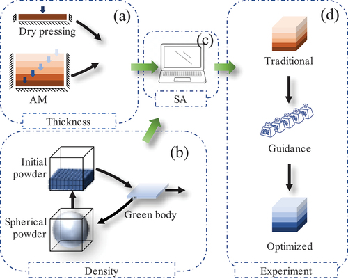
The research methodology of this article is as follows: The density of the AM ceramic green body is initially calculated using a new DSE model. Subsequently, this density distribution is further optimized through the application of the SA method. Thereafter, the efficacy of the optimized scheme is empirically validated via a series of experiments, as depicted in Figure 1.

Figure 1. (a) Derivation of the thickness of dry-pressed green body by Maxwell’s model, later generalized to AM green body. (b) Establishing the connection between the macroscopic force and the microstructure of green body through the DSE model, and then obtaining the density. (c) The results of thickness and density are subjected to SA to obtain an optimized pressure solution. (d) Experimental verification of the density uniformity of the laser ceramics before and after optimization.

2.1. Thickness calculated by Maxwell model

Ceramic particles are viscoelastic materials, with compressibility like gas, fluidity-like liquid, and resistance to deformation-like solids, usually calculated by Maxwell model. Based on Maxwell model, the nth layer thickness of AM green body is deduced in Appendix A.

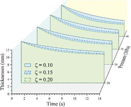
The theoretical thickness of the ceramic green body is depicted in Figure 2. As time increases, the thickness of the green body decreases, exhibiting an exponential trend. The rate of reduction initially is rapid, subsequently diminishing until the thickness stabilizes at a constant value. Furthermore, the rate of decrease is influenced by the pressure and the attenuation coefficient. Specifically, the greater the pressure applied to the green body, the faster the rate of reduction. Similarly, a larger attenuation coefficient correlates with a swifter reduction rate. The attenuation coefficient is a constant inherent to the ceramic material. In other words, the thickness of the ceramic is related to external factors such as pressure, as well as internal factors, including the attenuation coefficient.

Figure 2. Theoretical thickness reduction with time of pressing and indenter pressure (the rate of thickness decay is positively correlated with indenter pressure and rate of decay, where the decay coefficient is a constant related to the properties of the powder).

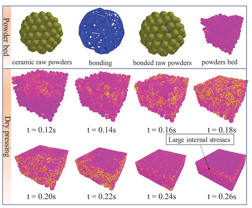
To verify the theoretical results of green body thickness and study the micro evolution of green body formation, this paper adopts the discrete element method (DEM) software to simulate the forming process, as shown in Figure 3. First, a simulation model is set up. The simulated ceramic particles are ceramic ball powders composed of smaller ceramic powders. The ceramic powders are connected by bonds, representing ceramic binders. The size ratio of ceramic powders and ceramic ball powders is based on the experimental compression shrinkage rate. Then, pressure is applied to the ceramic powders. At the beginning of compression, the green body is a soft particle bed composed of ceramic ball powders. During compression, the top particles are crushed under pressure, and the resulting fragments fill the larger gaps. Subsequently, the lower particles are crushed. Finally, all broken ceramic powders are extruded into a cube. The thickness results show that the simulated thickness is consistent with the theoretical thickness, both showing exponential decay. The microstructure shows that the green body near the mold wall and the pressing head bears greater stress, which means that the density of the green body near the mold wall and the pressing head is high.

Figure 3. The DEM software simulates dry-pressed ceramic green body in which the powder is crushed from top to bottom (the red, green and blue colors of the balls represent the internal stresses from large to small, respectively).

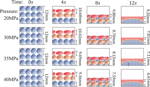
Combining the theoretical results and simulation results, this paper presents a schematic diagram of the pressed green body, as shown in Figure 4. The pressing process can be structured into three stages: crushing, filling, and extrusion. At t = 0, the ceramic particles are in a relaxed state. Before 4 s, the ceramic ball powders under pressure begin to deform, crack, and are about to crush. The closer to the mold wall and pressing head, the greater the degree of deformation and the more likely to crush. Between 4–8 s, the upper layer particles crush, and the crushed ceramic powders fall into the gaps of the lower layer particles. Between 8-12s, all particles crush, and all ceramic powders are extruded. The density of the ceramic green body is high around the perimeter and low in the center.

Figure 4. Schematic diagram of a dry-pressed green body and the three states of powder: crushed, filled and extruded (the red, orange and blue colors represent internal stresses from large to small, respectively).

2.2. Density calculated by DSE model

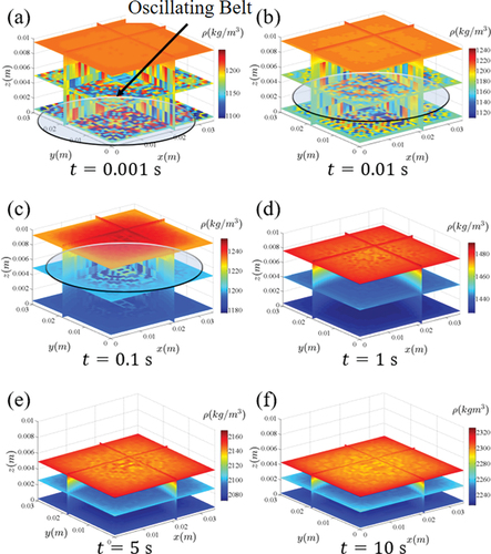
The simulation process is not clear enough to reflect the microscopic evolution and the laws of physical quantities. Based on molecular dynamics, a DSE model is designed (Appendix B). The characteristic of this model is that the microstructure of the green body can be deduced from the macroscopic force field, as shown in Figure 5. At 0.001 s, the height of the green body remains unchanged, but microstructural changes are evident. Specifically, sharp oscillatory belt appears in the lower part of the green body. During compression, there are macro- and micro-changes in the ceramic. Macroscopically, the thickness gradually decreases and stabilizes at a certain height, consistent with previous theoretical and simulation results. Microscopically, the density oscillatory belt shift upward and gradually disappears. The final density distribution exhibits high density around the perimeter and low density in the center. The DSE model calculations and DEM simulations exhibit a striking congruence between the micro-scale oscillations and the macroscopic density distribution.

Figure 5. Density of AM green body with five-layer structure calculated by DSE model: 1, the belt of particle oscillations shifts upward with time; 2, the thickness of green body decays exponentially with time; and 3, the final density of green body which near the wall and at the top is greatest.

2.3. Density optimization through SA algorithm

In 1953, Metropolis proposed a meta-heuristic optimization algorithm, Simulated Annealing (SA) algorithm, based on the inspiration of metal annealing, suitable for solving large-scale combinatorial problems [31].

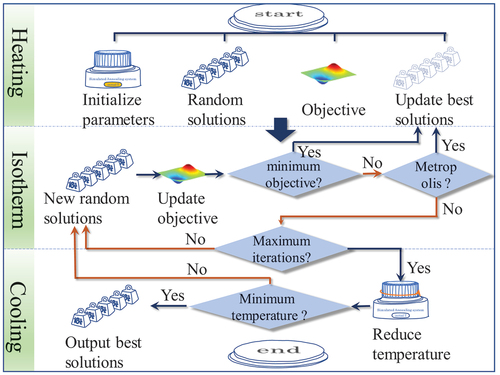
The Simulated Annealing (SA) algorithm’s procedural flow is delineated in Figure 6, encompassing three pivotal stages: heating, isothermal, and cooling. During the heating phase, the SA algorithm is initialized, establishing both arbitrary initial and tentative optimal pressure values. The isothermal phase involves numerous optimization iterations conducted at a constant temperature, yielding solutions that more closely align with the objective function presented in Appendix C. Notably, temperature serves as a critical parameter within SA, dictating the range of stochastic pressure variations and the tolerance for suboptimal solutions. As the process transitions to the cooling phase, the temperature is incrementally reduced, thereby narrowing the scope of stochastic perturbations and diminishing the likelihood of accepting inferior solutions, ultimately steering the optimization outcomes toward stability and convergence.

Figure 6. The flowchart of SA consists of 1, a heating phase to initialize the SA parameters; 2, an isotherm phase to find the optimal solution at a certain temperature; and 3, a cooling phase to converge the optimal solution and improve the accuracy of the optimal solution.

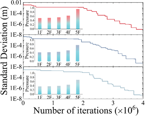
There is the density standard deviation with the number of iterations as shown in Figure 7 (subplot, showing the final guidance pressure). The effectiveness of the optimization can be seen in the fact that the standard deviation of the density decreases by 6 orders of magnitude after $4\times {10}^6$ computer iterations from the three optimization results. The guided pressure shows an increasing trend with the number of layers pressed, with the first four layers increasing within 10% and the last pressure increasing by about 30%.

Figure 7. The results of the SA optimization converge: the standard deviation is reduced by 6 orders of magnitude (the subplot is the gradient pressure increasing with the number of layers).

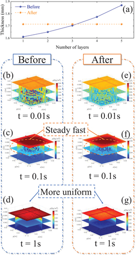
This paper compares the thickness and density of the green body before and after optimization, as shown in Figure 8. The pressures are all 15 MPa before optimization and (18, 18.36, 19.31, 22.08, 33.02) MPa after optimization. The results indicate that, under the traditional pressing process, the green body exhibits an uneven thickness, with a thinner bottom layer and thicker upper layer. However, after implementing an optimized gradient pressing process, the thickness of each layer tends to be more consistent, significantly enhancing thickness uniformity (Figure 8a). The results also show that on the one hand the optimized particles are stabilized faster and on the other hand the density variability of the optimized billets is less (Figure 8(b-g)). These show that there is an improved effect on the uniformity of density by the optimization scheme.

Figure 8. (a) Calculated thickness before and after optimization. (b-g) Calculated density before and after optimization (where (b,e) represents time t = 0.01 s, (c,f) represents time t = 0.1 s, and (d,g) represents time t = 1 s). The optimization is resulted in uniform thickness of the layers of the green body, faster particle stabilization, and higher density uniformity.

3. Experiment

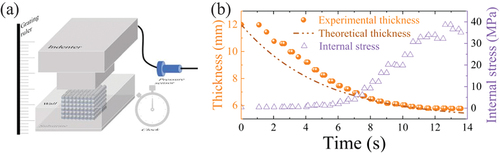
Ceramic powders are prepared by mixing α-Al₂O₃ (99.99%, Alfa Aesar, Tewksbury, MA, USA), Y₂O₃ (99.99%, Alfa Aesar, Tewksbury, MA, USA), and Yb₂O₃ (99.99%, Alfa Aesar, Tewksbury, MA, USA). In order to make the thermal distribution of laser ceramics more uniform, the doping concentrations of Yb are selected as 0.22at%, 0.32at% and 0.42at% [32]. Ceramic green bodies are formed under different pressures and holding times. After cold isostatic pressing under 200MPa for 2 min, the density of the green bodies became further uniform. Figure 9 illustrates the thickness and internal stress of a dry pressed green body over time, where the data for the thickness are from the grating ruler and the data for the internal stress is from the pressure sensor. Firstly, the experimental and theoretical thickness show an exponential decay with time. Secondly, the internal stress increases slowly with time, which is due to the crushing and filling of the ceramic ball powder in batches. Finally, the transient change in internal stress is approximately 0.1 s later than the transient change in height, which is the stress relaxation of the transition from the oscillatory to the steady state after particle crushing. These experimental phenomena are consistent with theoretical predictions. The difference with the theory is that the experimental stress relaxation occurs multiple times, while the theoretical stress relaxation occurs once.

Figure 9. (a) Mold for pressing powder and system for collecting data, (b)The thickness and internal stress of a dry pressed green body over time.

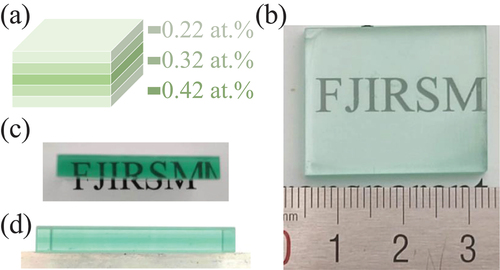
Figure 10 shows macroscopic morphology of the laser ceramics before annealing: (a) schematic diagram of the five-layer structure, (b) macroscopic photograph of the front face of the laser ceramics, (c) macroscopic photograph of the side face of the laser ceramics, and (d) photograph of the laser ceramics through natural light. Considering more uniform heat power and concentration diffusion distance, a five-layer structure with symmetrical concentration is designed in this paper. Each layer has a thickness of 1 mm. The sintered ceramic has a length of approximately 28 mm and a width of approximately 22 mm. The ceramic exhibits a light green color due to the doping of Yb, with a darker color in the middle layer and lighter colors in the upper and lower layers. Under natural light, the ceramic exhibits a clear five-layer structure with flat boundaries between layers, indicating that the experimental samples meet high-precision standards and design requirements.

Figure 10. Macroscopic morphology of the laser ceramics before annealing: (a) schematic diagram of the five-layer structure, (b) macroscopic photograph of the front face of the laser ceramics, (c) macroscopic photograph of the side face of the laser ceramics, and (d) photograph of the laser ceramics through natural light.

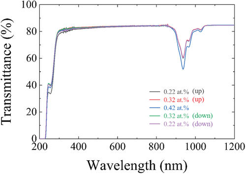
The optical properties of various parts of the ceramic are shown in Figure 11. The transmittance of different parts of the ceramic is measured in this paper. In the visible light band, ceramics with various concentrations have similar transmittance, all exceeding 84%. Near 940 nm, the ceramic exhibits a characteristic absorption peak of Yb. The higher the doping concentration of Yb, the lower the transmittance of the ceramic. This indicates good optical properties of the ceramic.

Figure 11. Transmittances of laser ceramic with five-layer structure.

Figure 12 shows scanning electron micrograph (SEM) of the thermally corroded surface within the annealed laser ceramic. Micrographs show ceramic grains ranging from 2 to 5 micrometers, indicating uniform grain size that enhances optical properties of polycrystalline materials. Numerous white dots appear at grain boundaries, revealed as deposited gold powder through electron microscopy analysis. The ceramic exhibits minimal porosity, reducing void scattering and further enhancing its optical performance.

Figure 12. Scanning electron micrograph (SEM) of the thermally corroded surface within the annealed laser ceramic.

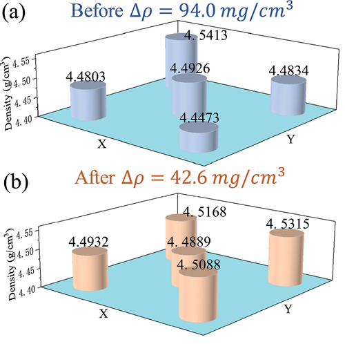
Figure 13 shows the experimental results of ceramic density before and after optimization, based on Archimedes densitometry. The results show that the maximum density difference of ceramics before optimization is 0.0940 g/cm³ and after optimization is 0.0426 g/cm³. Density uniformity has been optimized to improve by 45%. The density in the northeast before optimization is high and the density in the southwest is low, which could be due to uneven spread of powder. After optimization, the density is high around and low in the center, which is consistent with the theoretical prediction.

Figure 13. (a) Density distribution before optimization and maximum density difference of 94.0 mg/cm³, (b), Density distribution after optimization and maximum density difference of 42.6 mg/cm³.

4. Conclusion

In this paper, we propose a new method to improve the density uniformity of AM laser ceramics. First, a new DSE model was designed. This model predicts the spatial and temporal distribution of the density in the ceramic green body during AM. The model takes into account parameters such as compaction pressure and duration, and reveals the phenomenon of oscillating bands of particle density, with a high-density area near the mold wall and indenter. The DSE model is validated by experimental measurements and simulation results. Then, combined with the DSE calculation results and SA algorithm optimization, a new process to improve the density uniformity was proposed with the pressure 18, 18.36, 19.31, 22.08, 33.02 MPa. The experimental results confirm that the optimized process significantly improves the density uniformity of the laser ceramics by 45%. The study also includes a comprehensive theoretical analysis of thickness calculations using the Maxwell model, as well as a detailed study of the evolution of the microstructure of the blank by DEM simulation. Laser ceramics with a more uniform density have improved optical properties and contributed to the development of high-energy solid-state lasers.

Author contributions

Conceptualization, Biwu Dong; Funding acquisition, Jing Deng, Jianhong Huang and Wenxiong Lin; Methodology, Biwu Dong and Shengmiao Feng; Project administration, Jing Deng, Shengmiao Feng, Jianhong Huang and Wenxiong Lin; Resources, Qiufeng Huang and Jian Chen; Software, Biwu Dong and Yuchao Wang; Supervision, Jing Deng, Shengmiao Feng, Jianhong Huang and Wenxiong Lin; Writing – original draft, Biwu Dong.

Disclosure statement

No potential conflict of interest was reported by the author(s).

Additional information

Funding

National Key Research and Development Program of China [2021YFB3502702].

Appendix A:

Maxwell model

1. Thickness by dry pressing

The Maxwell model is expressed as:

(A1) $\mathit{\sigma }=\mathit{E\epsilon }\left(\mathit{t}\right)+\mathit{C}\dot{\epsilon }\left(\mathit{t}\right)$(A1)

where $\mathit{\sigma }$ is the stress. $\mathit{E}=60\mathit{MPa}$ represents the elastic modulus of green body. $\mathit{\epsilon }\left(\mathit{t}\right)$ represents the strain of green body at time t. $\mathit{C}$ is the viscous damping coefficient of the ceramic. The moment when the ceramic ball powder is just under pressure is defined as the initial moment. The initial strain at this point

(A2) $\mathit{\epsilon }\left(0\right)=0$(A2)

The time evolution of the strain is obtained by the first-order differential equation (A1).

(A3) $\mathit{\epsilon }\left(\mathit{t}\right)=\frac{\sigma }{E}\left(1-e^{-\mathit{\varsigma t}}\right)$(A3)

where $\mathit{\varsigma }$ is the strain attenuation coefficient, which is related to both the elastic modulus and viscosity coefficient of the green body.

(A4) $\mathit{\varsigma }=\frac{E}{C}$(A4)

equation (A3)(A3) $\mathit{\epsilon }\left(\mathit{t}\right)=\frac{\sigma }{E}\left(1-e^{-\mathit{\varsigma t}}\right)$(A3) shows that strain increases infinitely as the stress increases at time tends to infinity. However, experiments (Figure 9) show that at time tends to infinity, the strain tends to a fixed value rather than continuing to increase.

While observing the experimental process, it is noted that as the pressing time increased, the voids of the particles are gradually filled. And when the grain gap is completely filled, the thickness of the green body does not reduction i.e., the void ratio determines the upper limit of the strain. Combined with the fitting line of dry pressing experiments, the porosity of the ceramic raw powder is obtained as $58\mathrm{\%}\sim 68\mathrm{\%}$, and the median value is selected as the model value $\mathit{\eta }=63\mathrm{\%}$. The improved strain becomes

(A5) $\mathit{\epsilon }\left(\mathit{t}\right)=\left\{\begin{array}{c}\frac{\sigma }{E}\left(1-e^{-\mathit{\varsigma t}}\right),\mathit{\epsilon }\left(\mathit{t}\right)<\mathit{\eta }\\ \mathit{\eta },\mathit{else}\end{array}\right.$(A5)

And the thickness of the dry pressing is:

(A6) $\mathit{h}\left(\mathit{t}\right)=h_0\left[1-\mathit{\epsilon }\left(\mathit{t}\right)\right]$(A6)

in which $h_0=12\mathit{mm}$ is the loose thickness of ceramic ball powder.

2. Thickness by AM

The process of AM is to spread ceramic powders several times in the mold and apply pressure and holding time to each layer. In order to calculate the thickness of different layers in the AM green body, replace nth physical time with the sum, i.e., effective time, of mth physical time and (m-1)th transitive time.

(A7) ${\mathrm{t}}_{\mathrm{mn}}=\left\{\begin{array}{c}\begin{array}{cc}{t}_m,& \mathit{n}=\mathit{m}\end{array}\\ \begin{array}{cc}{t}_m+T_{\mathit{m}-1},& \mathit{n}<\mathit{m}\end{array}\end{array}\right.$(A7)

were $t_{\mathit{mn}}$ represents the nth effective time of the total m layer, and $t_m$ represents the mth holding time, and $T_{\mathit{m}-1}$ represents the (m-1)th transitive time. Transitive time is to transfer the compression effect of the nth layer to the next layer in the form of time.

(A8) $\mathit{h}\left({\sigma }_n,t_{\mathit{mn}}\right)=\mathit{h}\left({\sigma }_{\mathit{n}+1},T_m\right)$(A8)

where ${\sigma }_n$ represents the nth pressure. Bring equations (A5, A6) into equation (A8) to solve the transitive time

(A9) $T_m=-\frac{1}{\varsigma }ln\left[1-\frac{{\sigma }_n}{{\sigma }_{\mathit{n}+1}}\left(1-e^{-\mathit{\varsigma }{\mathit{t}}_{\mathit{mn}}}\right)\right]$(A9)

get the thickness of different layers in the AM green body

(A10) $h_n\left(\mathit{t}\right)=h_{\mathit{n}0}\left[1-{\epsilon }_n\left(t_{\mathit{mn}}\right)\right]$(A10)

in which $h_{\mathit{n}0}=2\mathit{mm}$ is the each loose thickness of each layer within green body.

Appendix B:

Density Spatiotemporal Evolution model (DSE)

1. Macroscopic force field

The AM uses a uniaxial vertical pressure, and the horizontal area remains unchanged, which is $X_0{Y}_0$, $X_0=35\mathit{mm},Y_0=30\mathit{mm}$. Macroscopic pressure on the upper surface of the green body

(B1) $F_{\mathit{up}}=F_0$(B1)

Macroscopic pressure on the down surface

(B2) $F_{\mathit{down}}=\mathit{\xi }{F}_0$(B2)

where $\mathit{\xi }$ represents the coefficient of the supporting force. During the pressing process, the mold wall creates a lateral pressure on the green body to resist expansion. This pressure includes a force from the x-direction (defined as the longer side)

(B3) $F_{\mathit{Nx}}=\mathit{\alpha }{F}_0$(B3)

and a force from the y-direction (defined as the shorter side)

(B4) $F_{\mathit{Ny}}=\mathit{\gamma }{F}_0$(B4)

where $\mathit{\alpha }$ and$\mathit{\gamma }\mathit{\hspace{0.17em}}$represent the lateral pressure coefficients in the x and y directions, respectively. The green body thickness is calculated by Appendix A: Maxwell model.

(B5) $\mathit{H}=\sum _{\mathit{n}=1}^m{h}_n\left(t_{\mathit{mn}}\right)$(B5)

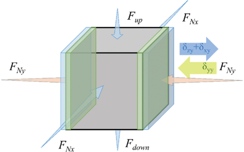
In a short period of time δ(t), thesuoli pressures $F_{\mathit{up}}$ and $F_{\mathit{down}}$ in the vertical direction of the green body cause the amount of its expansion in the y-direction to be δzy (Figure B1).

Figure B14. Schematic diagram of the force deformation in the y direction of the compact.

(B6) ${\delta }_{\mathit{zy}}=\mathrm{u}\frac{F_0+\mathit{\xi }{F}_0}{\mathit{E}{X}_0{Y}_0}$(B6)

where u is the Poisson’s ratio. Suppose that the side pressure $F_{\mathit{Nx}}$ in the x-direction of the green body causes its expansion in the y-direction to be ${\delta }_{\mathit{xy}}$ in the same amount of time.

(B7) ${\delta }_{\mathit{xy}}=\mathit{u}\frac{2\alpha F_0}{\mathit{E}{Y}_0\mathit{H}}$(B7)

At the same time, the side pressure $F_{\mathit{Ny}}$ in the y-direction of the green body causes its compression in the y-direction to be ${\delta }_{\mathit{yy}}$.

(B8) ${\delta }_{\mathit{yy}}=\frac{2\gamma F_0}{\mathit{E}{X}_0\mathit{H}}$(B8)

Since the horizontal area of the blank does not change during uniaxial pressing, the amount of expansion in the y- direction is equal to the amount of compression (Figure B1).

(B9) ${\delta }_{\mathit{yy}}={\delta }_{\mathit{zy}}+{\delta }_{\mathit{xy}}$(B9)

Bring Eqs. (B.6-B.8) into equation (B.9)

(B10) $2\mathit{\gamma }{F}_0{Y}_0=\mathit{u}\left(F_0+\mathit{\xi }{F}_0\right)\mathit{H}+2\mathit{u\alpha }{F}_0{X}_0$(B10)

The relation of extrusion expansion in the x-direction is obtained similarly

(B11) $2\mathit{\alpha }{F}_0{X}_0=\mathit{u}\left(F_0+\mathit{\xi }{F}_0\right)\mathit{H}+2\mathit{u\gamma }{F}_0{Y}_0$(B11)

using Eqs. (B10, B11) obtain the lateral pressure coefficient in the x-direction

(B12) $\mathit{\alpha }=\frac{\mathit{u}\left(1+\mathit{\xi }\right)H}{2\left(1-\mathit{u}\right)X_0}$(B12)

and the lateral pressure coefficient in the y-direction

(B13) $\mathit{\gamma }=\frac{\mathit{u}\left(1+\mathit{\xi }\right)H}{2\left(1-\mathit{u}\right)Y_0}$(B13)

2. Microscopic force field

The structure of ceramic particles is also loose, similar to that of gas, and there are no strong chemical bonds between the particles. Therefore, the magnitude of the conduction force is affected by the distance traveled. At the microscopic level, as the distance between the particles and the mold increases, the pressure gradually decreases. Now coordinates of a ceramic ball are $\left(\mathit{X},\mathit{Y},\mathit{Z}\right)$, and its particle size is $\mathit{\varphi }$. The outer cube of ceramic ball is $\left(x_0,y_0,z_0\right)$. The pressure on the upper of the ceramic ball is

(B14) $F_{\mathit{up}}=-{\mathrm{f}}_z{e}^{-{\lambda }_{\mathrm{\perp }}\left(\mathit{H}-\mathit{Z}\right)}{\hat{e}}_{\mathit{z}}$(B14)

At this time, the pressure on the down of ceramic ball is

(B15) $F_{\mathit{down}}=\mathit{\xi }{f}_z{e}^{-{\lambda }_{\mathrm{\perp }}\mathit{Z}}{\hat{e}}_{\mathit{z}}$(B15)

Lateral pressure in the x-direction of the wall

(B16) $F_{\mathit{Nx}}=\mathit{\alpha }{f}_x{e}^{-{\lambda }_{\parallel }{l}_X}{\hat{e}}_{\mathit{x}}$(B16)

and lateral pressure in the y-direction

(B17) $F_{\mathit{Ny}}=\mathit{\gamma }{\mathrm{f}}_y{e}^{-{\lambda }_{\parallel }{l}_Y}{\hat{\mathrm{e}}}_{\mathit{y}}$(B17)

where $\left({\lambda }_{\mathrm{\perp }}=233m^{-1},{\lambda }_{\parallel }=233m^{-1}\right)$ denotes the attenuation coefficients of the force in the vertical and horizontal directions, respectively. $\left({\hat{e}}_{\mathit{x}},{\hat{e}}_{\mathit{y}},{\hat{e}}_{\mathit{z}}\right)$ represent unit vectors in the direction of x, y, and z, respectively.$\left(l_X=\frac{X_0}{2}-\left|\mathit{X}-\frac{X_0}{2}\right|,l_Y=\frac{Y_0}{2}-\left|\mathit{Y}-\frac{Y_0}{2}\right|\right)$ represents the shortest distance of ceramic ball powder from the sidewall in the x direction and y direction, respectively. $\left(f_x,f_y,f_z\right)$ are the projections of the macroscopic force field in the three directions, respectively.

(B18) $f_x=\frac{F_0{y}_0{z}_0}{Y_0\mathit{H}}$(B18)

(B19) $f_y=\frac{F_0{x}_0{z}_0}{X_0\mathit{H}}$(B19)

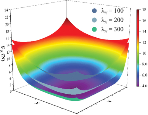
and

(B20) $f_z=\frac{F_0{x}_0{y}_0}{X_0{Y}_0}$(B20)

The lateral pressure is lower in the middle, and higher in the periphery, showing a valley conical distribution (Figure B2). In addition, as the horizontal attenuation coefficient increases, the pressure value decay rate from the sidewall to the center will accelerate.

Figure B15. Spatial distribution of lateral pressure.

On the down surface of the green body, the pressure and support forces are equal in magnitude and opposite in direction.

(B21) $F_{\mathit{up}}{|}_{\mathcal{Z}=0}+F_{\mathit{down}}{|}_{\mathcal{Z}=0}=0$(B21)

Bringing equations (B14, B15) into equation (B21), the conversion coefficient of the support force is

(B22) $\mathit{\xi }=e^{-{\lambda }_{\mathrm{\perp }}\mathit{H}}$(B22)

Ceramic particles are subjected to a vertical upward friction force.

(B23) $F_{\mu }=\mathit{\mu }\sqrt{{{\mathit{F}}_{\mathit{Nx}}}^2+{{\mathit{F}}_{\mathit{Ny}}}^2}$(B23)

in which, $\mathit{\mu }$ represents the coefficient of friction between the ceramic particles and the steel mold. The adhesive force between the ceramic particles hinders those relative movement. Newton believed that viscous force was directly proportional to the mold contact area and flow velocity, and inversely proportional to the distance.

(B24) $F_{\nu }=\mathit{qA}\frac{\dot{z}}{\mathit{l}}$(B24)

where $\mathit{q}$ is the dynamic viscosity coefficient of the ceramic particles. $\mathit{A}$ is the area of the fixed mold, which is parallel to the direction of movement. $\mathit{l}$ is the distance between particles and fixed wall. Analyze the viscous force in the y-direction, and the projection area of the ceramic particle in the $\mathit{xoz}$ plane is

(B25) $\mathit{A}=x_0\left(z_0-\mathit{z}\right)$(B25)

The distance of the ceramic particle from the mold wall is

(B26) $\mathit{l}=l_Y+\mathit{\varphi }$(B26)

There is a positive correlation between dynamic viscosity $\mathit{q}$and density, as measured by kinematic viscosity $\mathit{\nu }$.

(B27) $\mathit{\nu }=\frac{q}{\rho }$(B27)

$\mathit{\rho }$ represents the density of the ceramic particle.

(B28) $\mathit{\rho }=\frac{M}{x_0{y}_0\left(z_0-\mathit{z}\right)}$(B28)

$\mathit{M}$ represents the quality of the ceramic particle. In summary, the viscous forces in the x and y directions are sum as

(B29) $F_v=\mathit{D}\dot{z}$(B29)

where $\mathit{D}$ is the viscous force coefficient

(B30) $\mathit{D}=\mathit{\nu M}\left[\frac{1}{x_0\left(l_X+\mathit{\varphi }\right)}+\frac{1}{y_0\left(l_Y+\mathit{\varphi }\right)}\right]$(B30)

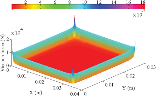
According to equation (B29(B29) $F_v=\mathit{D}\dot{z}$(B29) and B30(B30) $\mathit{D}=\mathit{\nu M}\left[\frac{1}{x_0\left(l_X+\mathit{\varphi }\right)}+\frac{1}{y_0\left(l_Y+\mathit{\varphi }\right)}\right]$(B30) ), the viscous force is positively correlated with the kinematic viscosity $\mathit{\nu }$, and negatively correlated with the particle size $\mathit{\varphi }$. The viscous force decays rapidly as the distance between the ceramic particle and the mold wall increases (Figure B3). This viscous force in the center of the mold is almost 0.

Figure B16. Viscous force distribution diagram.

According to the different properties of ceramic particles, their elastic force can be divided into ceramic ball powder elasticity and ceramic raw powder elasticity.

(B31) $F_k=\left\{\begin{array}{c}{k}_B\mathit{z},\mathit{ball}\mathit{power}\\ k_b\mathit{z},\mathit{raw}\mathit{power}\end{array}\right.$(B31)

Here, $k_B$ and $k_b$ denote the Hooke coefficients of ceramic ball powder and ceramic raw powder, respectively.

3. Microscopic movement

Ceramic ball powder under pressure creates a counter-stress. When stress is greater than the critical threshold, ceramic ball powder is crushed into ceramic raw powder. The crushed raw powder then falls under pressure, and fills the loose gaps of the microscopic cube. Finally, after the gap is completely filled, the raw powder is deformed by force. Therefore, according to the different morphology and movement state of ceramic particles, the pressing process is divided into three stages: crushing, filling and extrusion.

3.1. Crushing of ceramic ball powder

The mechanical equation of ball powder is

(B32) $\left\{\begin{array}{c}{F}_x=F_{\mathit{Nx}}-k_B{x}_a\\ F_y=F_{\mathit{Ny}}-k_B{y}_a\\ F_z=-F_{\mathit{up}}+F_{\mathit{down}}+F_{\mu }-F_{\nu }-k_B{z}_a\end{array}\right.$(B32)

where $\left(x_a,y_a,z_a\right)$ are the displacements of ceramic ball powder in three directions, respectively. The motion equation of ball powder obtained by Newtonian dynamics:

(B33) $\left\{\begin{array}{c}\mathit{M}{\ddot{x}}_{\mathit{a}}-F_{\mathit{Nx}}+k_B{x}_a=0\\ \mathit{M}{\ddot{y}}_{\mathit{a}}-F_{\mathit{Ny}}+k_B{y}_a=0\\ \mathit{M}{\ddot{z}}_{\mathit{a}}+F_{\mathit{up}}-F_{\mathit{down}}-F_{\mu }+\mathit{D}{\dot{z}}_{\mathit{a}}+k_B{z}_a=0\end{array}\right.$(B33)

Those are second-order differential equations, and their boundary conditions are:

(B34) $\left\{\begin{array}{c}{x}_a\left(0\right)=0;{x_a}^{\prime }\left(0\right)=0\\ y_a\left(0\right)=0;{y_a}^{\prime }\left(0\right)=0\\ z_a\left(0\right)=0;{z_a}^{\prime }\left(0\right)=0\end{array}\right.$(B34)

solve those equations to obtain the motion of ball powder.

(B35) $\left\{\begin{array}{c}{x}_a\left(\mathit{t}\right)=\frac{{\mathit{F}}_{\mathit{Nx}}}{k_B}\left[1-cos\left(\mathit{\omega t}\right)\right]\\ y_a\left(\mathit{t}\right)=\frac{{\mathit{F}}_{\mathit{Ny}}}{k_B}\left[1-cos\left(\mathit{\omega t}\right)\right]\\ z_a\left(\mathit{t}\right)=\frac{{\mathit{F}}_{\mathit{up}}-F_{\mathit{down}}-F_{\mu }}{2k_B}\left[\left(1+\mathit{\varrho }\right)e^{-{\lambda }_1\mathit{t}}+\left(1-\mathit{\varrho }\right)e^{-{\lambda }_2\mathit{t}}-2\right]\end{array}\right.$(B35)

in which

(B36) $\left\{\begin{array}{c}{\lambda }_1=\mathit{\beta }-\sqrt{{\beta }^2-{\omega }^2}\\ {\lambda }_1=\mathit{\beta }+\sqrt{{\beta }^2-{\omega }^2}\end{array}\right.$(B36)

and

(B37) $\left\{\begin{array}{c}\mathit{\omega }=\sqrt{\frac{k_B}{\mathit{M}}}\\ \mathit{\beta }=\frac{D}{2\mathit{M}}\\ \mathit{\varrho }=\frac{\beta }{\sqrt{{\beta }^2-{\omega }^2}}\end{array}\right.$(B37)

3.2. Moment of crushing

Stress of ball powder

(B38) ${\sigma }^{\mathit{a}}\left(\mathit{t}\right)=\frac{x_a\left(\mathit{t}\right)E_x}{x_0}{\hat{\mathrm{e}}}_{\mathit{x}}+\frac{y_a\left(\mathit{t}\right)E_y}{y_0}{\hat{\mathrm{e}}}_{\mathit{y}}+\frac{z_a\left(\mathit{t}\right)E_z}{z_0}{\hat{\mathrm{e}}}_{\mathit{z}}$(B38)

with Elastic Modulus

(B39) $\left\{\begin{array}{c}{E}_x=\frac{k_B{x}_0}{y_0{z}_0}\\ E_y=\frac{k_B{y}_0}{x_0{z}_0}\\ E_z=\frac{k_B{z}_0}{x_0{y}_0}\end{array}\right.$(B39)

Since the critical threshold is much smaller than the pressure, the time before crushing is very short. The movement of ball powder could be unfolded in Taylor at zero time.

(B40) $\left\{\begin{array}{c}\underset{\mathit{t}\to 0}{lim}{x}_a\left(\mathit{t}\right)=\frac{{\mathit{F}}_{\mathit{Nx}}}{2\mathit{M}}{t}^2\\ \underset{\mathit{t}\to 0}{lim}{y}_a\left(\mathit{t}\right)=\frac{{\mathit{F}}_{\mathit{Ny}}}{2\mathit{M}}{t}^2\\ \underset{\mathit{t}\to 0}{lim}{z}_a\left(\mathit{t}\right)=-\frac{\left({\mathit{F}}_{\mathit{up}}-F_{\mathit{down}}-F_{\mu }\right)}{2\mathit{M}}{t}^2\end{array}\right.$(B40)

Get the stress after unfolding

(B41) ${\sigma }_a\left(\mathit{t}\right)=\frac{k_B{F}_{\mathrm{\Gamma }}{t}^2}{2{\varphi }^2\mathit{M}}$(B41)

here

(B42) $F_{\mathrm{\Gamma }}=\sqrt{F_{Nx}^2+F_{Ny}^2+{\left({\mathit{F}}_{\mathit{up}}-F_{\mathit{down}}-F_{\mu }\right)}^2}$(B42)

Ball powder breaks when the stress is equal to the critical strength $\left|{\mathit{\sigma }}^a\left(t_a\right)\right|={\sigma }_B$.

(B43) $t_a=\sqrt{\frac{2{\varphi }^2\mathit{M}{\sigma }_B}{k_B{F}_{\mathrm{\Gamma }}}}$(B43)

3.3. Ceramic raw powder fills the voids

the mechanical equation of ceramic raw powder is

(B44) $F_z=-F_{\mathit{up}}-F_{\mathit{down}}-F_{\mathrm{k}}$(B44)

The motion equation of raw powder obtained by Newtonian dynamics

(B45) $\mathit{M}{\ddot{z}}_{\mathit{b}}+F_{\mathit{up}}+F_{\mathit{down}}+\mathit{D}{\dot{z}}_{\mathit{b}}=0$(B45)

this is also second-order differential equation, and its boundary condition is:

(B46) $z_b\left(t_a\right)=0;z_b^{\prime }\left(t_a\right)=0$(B46)

solve this equation to obtain the motion of raw powder.

(B47) $z_b\left(\mathit{t}\right)=\frac{{\mathit{F}}_{\mathit{up}}+F_{\mathit{down}}}{\mathit{D\tau }}\left[1-\mathit{\tau }\left(\mathit{t}-t_a\right)-e^{-\tau \left(t-t_a\right)}\right]$(B47)

here

(B48) $\mathit{\tau }=\frac{D}{M}$(B48)

3.4. The moment of complete filling

The void displacement of the raw powder is

(B49) $\mathrm{\Delta }\mathit{z}=\frac{\mathrm{\Delta v}}{x_0{y}_0}=\mathit{\eta \varphi }$(B49)

where $\mathrm{\Delta v}$ is the void volume of the raw powder, and $\mathit{\eta }$ is the porosity, which is time-dependent.

(B50) $\mathit{\eta }={\eta }_{\mathit{max}}\left(1-e^{-\mathit{\chi t}}\right)$(B50)

Among them, ${\eta }_{\mathit{max}}=45\mathrm{\%}$ represents the porosity of all the ball powders after they are broken, i.e., the maximum porosity of ceramic raw powder. And $\mathit{\chi }=0.5$ is the porosity growth coefficient. The moment when the void is filled up is

(B51) $\left|z_b\left(t_b\right)\right|=\mathrm{\Delta }\mathit{z}$(B51)

Bring equation (B47) into equation (B51), expand the trigonometric term using Taylor formula, and pick the first three terms of the expansion.

(B52) $t_b=t_a+\sqrt{\frac{2\mathrm{\Delta }zM}{\left|{\mathit{F}}_{\mathit{up}}+F_{\mathit{down}}\right|}}$(B52)

3.5. Pressing of ceramic raw powder

The mechanical equation of raw powder is

(B53) $\left\{\begin{array}{c}{F}_x=F_{\mathit{Nx}}-k_b{x}_c\\ F_y=F_{\mathit{Ny}}-k_b{y}_c\\ F_z=-F_{\mathit{up}}+F_{\mathit{down}}+F_{\mu }-F_{\nu }-k_b{z}_c\end{array}\right.$(B53)

The motion equation of raw powder obtained by Newtonian dynamics:

(B54) $\left\{\begin{array}{c}\mathit{M}{\ddot{x}}_{\mathit{c}}-F_{\mathit{Nx}}+k_b{x}_c=0\\ \mathit{M}{\ddot{y}}_{\mathit{c}}-F_{\mathit{Ny}}+k_b{y}_c=0\\ \mathit{M}{\ddot{z}}_{\mathit{c}}+F_{\mathit{up}}-F_{\mathit{down}}-F_{\mu }+\mathit{D}{\dot{z}}_{\mathit{c}}+k_b{z}_c=0\end{array}\right.$(B54)

Those are also second-order differential equations, and their boundary conditions are:

(B55) $\left\{\begin{array}{c}{x}_c\left(t_b\right)=0;\wedge {x_c}^{\prime }\left(t_b\right)=0\\ y_c\left(t_b\right)=0;\wedge {y_c}^{\prime }\left(t_b\right)=0\\ z_c\left(t_b\right)=0;\wedge {z_c}^{\prime }\left(t_b\right)={z_b}^{\prime }\left(t_b\right)\end{array}\right.$(B55)

solve those equations to obtain the motion of raw powder.

(B56) $\left\{\begin{array}{c}{x}_c\left(\mathit{t}\right)=\frac{{\mathit{F}}_{\mathit{Nx}}}{k_b}\left[1-cos\left(\mathit{\varpi }\left(\mathit{t}-t_b\right)\right)\right]\\ y_c\left(\mathit{t}\right)=\frac{{\mathit{F}}_{\mathit{Ny}}}{k_b}\left[1-cos\left(\mathit{\varpi }\left(\mathit{t}-t_b\right)\right)\right]\\ z_c\left(\mathit{t}\right)=\frac{{\mathit{F}}_{\mathit{up}}-F_{\mathit{down}}-F_{\mu }}{k_b}\left\{e^{-\beta \left(t-t_b\right)}\frac{cos\left[\theta \left(t-t_b\right)-\mathit{\vartheta }\right]}{cos\left(\mathit{\vartheta }\right)}-1\right\}\\ +\frac{zb\left(t_b\right)e^{-\beta \left(t-t_b\right)}}{\mathit{\theta }}sin\left[\mathit{\theta }\left(\mathit{t}-t_b\right)\right]\end{array}\right.$(B56)

in which

(B57) $\left\{\begin{array}{c}\mathit{\varpi }=\sqrt{\frac{k_b}{\mathit{M}}}\\ \mathit{\theta }=\sqrt{{\varpi }^2-{\beta }^2}\\ \mathit{\vartheta }=\arctan \left(\frac{\beta }{\theta }\right)\end{array}\right.$(B57)

4. Density

The density of green body by dry pressing is calculated by displacement

(B58) $\mathit{\rho }\left(\mathit{t}\right)=\frac{M}{x_0{y}_0\left[z_0-\mathit{z}\left(\mathit{t}\right)\right]}$(B58)

where the displacement is

(B59) $\mathit{z}\left(\mathit{t}\right)=\left\{\begin{array}{c}\frac{{\mathit{F}}_{\mathit{up}}-F_{\mathit{down}}-F_{\mu }}{2k_B}\left[\left(1+\mathit{\varrho }\right)e^{-{\lambda }_1\mathit{t}}+\left(1-\mathit{\varrho }\right)e^{-{\lambda }_2\mathit{t}}-2\right],0\le t_a\\ z_a\left(t_a\right)+\frac{{\mathit{F}}_{\mathit{up}}+F_{\mathit{down}}}{\mathit{D\tau }}\left[1-\mathit{\tau }\left(\mathit{t}-t_a\right)-e^{-\tau \left(t-t_a\right)}\right],t_a\le t_b\\ z_a\left(t_a\right)+z_b\left(t_b\right)+\frac{{\mathit{F}}_{\mathit{up}}-F_{\mathit{down}}-F_{\mu }}{k_b}\left\{e^{-\beta \left(t-t_b\right)}\frac{cos\left[\theta \left(t-t_b\right)-\mathit{\vartheta }\right]}{\mathit{cos}\left(\mathit{\vartheta }\right)}-1\right\}\\ +\frac{zb\left(t_b\right)e^{-\beta \left(t-t_b\right)}}{\mathit{\theta }}\mathit{sin}\left[\mathit{\theta }\left(\mathit{t}-t_b\right)\right],\mathit{t}\ge t_b\end{array}\right.$(B59)

In order to calculate the density of different layers in the AM green body, replace nth physical time with the sum, i.e., effective time, of mth physical time and (m-1)th transitive time.

(B60) ${\mathrm{t}}_{\mathrm{mn}}=\left\{\begin{array}{c}\begin{array}{cc}{t}_m,& \mathit{n}=\mathit{m}\end{array}\\ \begin{array}{cc}{t}_m+T_{\mathit{m}-1},& \mathit{n}<\mathit{m}\end{array}\end{array}\right.$(B60)

were $t_{\mathit{mn}}$ represents the nth effective time of the total m layer, and $t_m$ represents the mth holding time, and $T_{\mathit{m}-1}$ represents the (m-1)th transitive time. Transitive time is to transfer the compression effect of the nth layer to the next layer in the form of time. To simplify the calculation of the transitive time, select the mechanical term, depth decay term, and time decay term in the displacement equation (B59).

(B61) $F_n{e}^{-{\lambda }_{\mathrm{\perp }}\left(H_{\mathit{mn}}-\mathit{Z}\right)}{e}^{-\mathit{\beta }{\mathit{t}}_{\mathit{mn}}}=F_{\mathit{n}+1}{e}^{-{\lambda }_{\mathrm{\perp }}\left(H_{\mathit{mn}+1}-\mathit{Z}\right)}{e}^{-\beta T_m}$(B61)

where $H_{\mathit{mn}}$ represents the thickness of the $\mathit{n}$ layer.

(B62) $\mathit{H}=\sum _{\mathit{i}=1}^n{h}_i$(B62)

Calculate the transitive time from equation (B61)

(B63) $T_m=t_{\mathit{mn}}-Q_n$(B63)

with

(B64) $Q_n=\frac{{\lambda }_{\mathrm{\perp }}{h}_{\mathit{n}+1}+ln\left(F_n/F_{\mathit{n}+1}\right)}{\mathit{\beta }}$(B64)

Bring Eqs. (B63, B64) into equation (B60) to solve the effective time

(B65) $t_{\mathit{mn}}=-\frac{{\lambda }_{\mathrm{\perp }}\left(H_{\mathit{mm}}-H_{\mathit{mn}}\right)+ln\left(F_n/F_m\right)}{\mathit{\beta }}+\sum _{\mathit{i}=\mathit{n}}^m{t}_i$(B65)

The density of green body by AM is

(B66) ${\rho }_n\left(t_{\mathit{mn}}\right)=\frac{M}{x_0{y}_0\left[z_0-\mathit{z}\left(t_{\mathit{mn}}\right)\right]}$(B66)

Appendix C:

Simulated annealing (SA)

To address the issue of uneven density in AM ceramics, we utilize a computational optimization approach based on SA, which is particularly effective for multi-variable nonlinear optimization problems. The objective function $f_{\mathit{obj}}$, a crucial component of SA, encompasses both a Maxwell model $f_{obj}^{\left(\mathit{high}\right)}$ for vertical density uniformity and a DSE model $f_{obj}^{\left(up\right)},f_{obj}^{\left(mid\right)},f_{obj}^{\left(\mathit{down}\right)}$ for horizontal density uniformity.

(C1) $f_{\mathit{obj}}=\mathit{r}{f}_{obj}^{\left(\mathit{high}\right)}+\mathit{u}{f}_{obj}^{\left(up\right)}+\mathit{v}{f}_{obj}^{\left(mid\right)}+\mathit{w}{f}_{obj}^{\left(\mathit{down}\right)}$(C1)

with weight factor $\mathrm{r}=0.5,\mathrm{u}=0.167,\mathrm{v}=0.167,\mathrm{w}=\mathrm{0.167.}$

(C2) $f_{obj}^{\left(\mathit{high}\right)}=\sqrt{\frac{1}{\mathit{m}-1}\sum _{\mathit{n}=1}^m{\left[h_n\left(t_{\mathit{mn}}\right)-\bar{h}\left(t_{\mathit{mn}}\right)\right]}^2}$(C2)

$\bar{h}\left(t_{\mathit{mn}}\right)$is the average of the thickness. Nine points are selected at each of the three heights (Figure C1) and are calculated the density using the DSE model to construct a density matrix.

Figure C17. Schematic diagram of the selection point of the density objective function.

(C3) ${\rho }_{\mathit{up}}=\left(\begin{array}{ccc}{\rho }_{\mathit{u}11}& {\rho }_{\mathit{u}12}& {\rho }_{\mathit{u}13}\\ {\rho }_{\mathit{u}21}& {\rho }_{\mathit{u}22}& {\rho }_{\mathit{u}23}\\ {\rho }_{\mathit{u}31}& {\rho }_{\mathit{u}32}& {\rho }_{\mathit{u}33}\end{array}\right)$(C3)

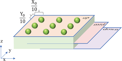
The standard deviation of a density matrix is calculated, which is the density objective function.

(C4) $f_{obj}^{\left(up\right)}=\mathit{std}\left({\rho }_{\mathit{up}}\right)$(C4)

Similarly, the density objective function for the middle is acquired, denoted as $f_{obj}^{\left(mid\right)}$, and the bottom, denoted as $f_{obj}^{\left(\mathit{down}\right)}$.

References

- Schawlow AL, Townes CH. Infrared and optical masers. Phys Rev. 1958;112(6):1940–1949. doi: 10.1103/PhysRev.112.1940
- Maiman TH. Stimulated optical radiation in Ruby. Nature. 1960;187(4736):493–494. doi: 10.1038/187493a0
- Liu H, Lin W, Hong M. Hybrid laser precision engineering of transparent hard materials: challenges, solutions and applications. Light Sci Appl. 2021;10(1):162. doi: 10.1038/s41377-021-00596-5
- Naresh, Khatak P. Laser cutting technique: a literature review. Mater Today Proc. 2022;56:2484–2489. doi: 10.1016/j.matpr.2021.08.250
- Han T, Nag A, Afsarimanesh N, et al. Laser-assisted printed flexible sensors: a review. Sensors. 2019;19(6):1462. doi: 10.3390/s19061462
- Betti R. A milestone in fusion research is reached. Nat Rev Phys. 2023;5(1):6–8. doi: 10.1038/s42254-022-00547-y
- Kobayashi J, Ogino A, Inouye S. Measurement of the variation of electron-to-proton mass ratio using ultracold molecules produced from laser-cooled atoms. Nat Commun. 2019;10(1):3771. doi: 10.1038/s41467-019-11761-1
- Forsythe RC, Cox CP, Wilsey MK, et al. Pulsed laser in liquids made nanomaterials for catalysis. Chem Rev. 2021;121(13):7568–7637. doi: 10.1021/acs.chemrev.0c01069
- Tsai C-T, Cheng C-H, Kuo H-C, et al. Toward high-speed visible laser lighting based optical wireless communications. Prog Quantum Electron. 2019;67:100225. doi: 10.1016/j.pquantelec.2019.100225
- Carrasco-Casado A, Shiratama K, Trinh PV, et al. Development of a miniaturized laser-communication terminal for small satellites. Acta Astronaut. 2022;197:1–5. doi: 10.1016/j.actaastro.2022.05.011
- Toyoshima M. Recent trends in space laser communications for small satellites and constellations. J Lightwave Technol. 2021;39(3):693–699. doi: 10.1109/JLT.2020.3009505
- Lyu C, Zhan R. STOP model development and analysis of an optical collimation system for a tactical high-energy laser weapon. Appl Optics. 2021;60(13):3596–3603. doi: 10.1364/AO.419554
- Bernatskyi A, Sokolovskyi M. History of military laser technology development in military applications. Hist Sci Technol. 2022;12(1):88–113. doi: 10.32703/2415-7422-2022-12-1-88-113
- Wang J, Cao L, Zhang Y, et al. Effect of mass transfer channels on flexural strength of C/SiC composites fabricated by femtosecond laser assisted CVI method with optimized laser power. J Adv Ceram. 2021;10(2):227–236. doi: 10.1007/s40145-020-0433-2
- Guo L, Xin H, Zhang Z, et al. Microstructure modification of Y2O3 stabilized ZrO2 thermal barrier coatings by laser glazing and the effects on the hot corrosion resistance. J Adv Ceram. 2020;9(2):232–242. doi: 10.1007/s40145-020-0363-z
- Liu H, Su H, Shen Z, et al. Formation mechanism and roles of oxygen vacancies in melt-grown Al2O3/GdAlO3/ZrO2 eutectic ceramic by laser 3D printing. J Adv Ceram. 2022;11(11):1751–1763. doi: 10.1007/s40145-022-0645-8
- Chen Z, Li Z, Li J, et al. 3D printing of ceramics: a review. J Eur Ceram Soc. 2019;39(4):661–687. doi: 10.1016/j.jeurceramsoc.2018.11.013
- Grossin D, Montón A, Navarrete-Segado P, et al. A review of additive manufacturing of ceramics by powder bed selective laser processing (sintering/melting): Calcium phosphate, silicon carbide, zirconia, alumina, and their composites. Open Ceramics. 2021;5:100073. doi: 10.1016/j.oceram.2021.100073
- Tian F, Jiang N, Liu Y, et al. Fabrication and properties of multistage gradient doping Yb: YAG laser ceramics. J Am Ceram Soc. 2023;106(4):2309–2316. doi: 10.1111/jace.18913
- Vajdi M, Sadegh Moghanlou F, Sharifianjazi F, et al. A review on the Comsol Multiphysics studies of heat transfer in advanced ceramics. J Of Compos And Compd. 2020;2(1):35–44. doi: 10.29252/jcc.2.1.5
- Hatch S, Parsons W, Weagley R. Hot‐pressed polycrystalline CaF2: Dy2+ laser. Appl Phys Lett. 1964;5(8):153–154. doi: 10.1063/1.1754094
- Greskovich C, Chernoch J. Polycrystalline ceramic lasers. J Appl Phys. 1973;44(10):4599–4606. doi: 10.1063/1.1662008
- Ikesue A, Kinoshita T, Kamata K, et al. Fabrication and optical properties of high‐performance polycrystalline Nd: YAG ceramics for solid‐state lasers. J Am Ceram Soc. 1995;78(4):1033–1040. doi: 10.1111/j.1151-2916.1995.tb08433.x
- Ikesue A, Aung YL. Ceramic laser materials. Nat Photonics. 2008;2(12):721–727. doi: 10.1038/nphoton.2008.243
- Li M, Hu H, Gao Q, et al. A 7.08-kW YAG/Nd: YAG/YAG composite ceramic slab laser with dual concentration doping. IEEE Photonics J. 2017;9(6):1–10. doi: 10.1109/JPHOT.2017.2780197
- al’nshin My B. The contact section of powder compacts and sintered bodies, and the values of their mechanical properties related to the contact section. Soviet Powder Metall Metal Ceram. 1964;2(4):278–281. doi: 10.1007/BF00774032
- Ge R. A new equation for powder compaction. Powder Metall Sci Technol. 1995;6:20–24.
- Kawakita K, Lüdde K-H. Some considerations on powder compression equations. Powder Technol. 1971;4(2):61–68. doi: 10.1016/0032-5910(71)80001-3
- Panelli R, Ambrozio Filho F. A study of a new phenomenological compacting equation. Powder Technol. 2001;114(1–3):255–261. doi: 10.1016/S0032-5910(00)00207-2
- Lun-Fu AV, Bubenchikov AM, Bubenchikov MA, et al. Computational analysis of strain-induced effects on the dynamic properties of C60 in fullerite. Crystals. 2022;12(2):260. doi: 10.3390/cryst12020260
- Metropolis N, Rosenbluth AW, Rosenbluth MN, et al. Equation of state calculations by fast computing machines. J Chem Phys. 1953;21(6):1087–1092. doi: 10.1063/1.1699114
- Xie J, Feng M, Han D, et al. Gradient doping composite multi-segmented slab lasers design optimization. Opt Laser Technol. 2024;168:109826. doi: 10.1016/j.optlastec.2023.109826