The geospatial modelling of carbon sequestration in Oluwa Forest, Ondo State, Nigeria

ABSTRACT

The study assessed the amount of carbon being sequestrated in the Ondo State Afforestation Project in Oluwa Forest, south -west of Nigeria, with the view to determine the above ground biomass (AGB) and belowground biomass (BGB), estimate the total carbon content and evaluate the CO₂ sequestered. Geospatial techniques and the non-destructive field observation method were used. The results showed that a total of 359 megatons of CO₂ was estimated to have been sequestered using the non-destructive field measurements. In addition, the rate of change in land use land cover between 1984 and 2015 was determined. A geospatial database derived from field measurements was developed to monitor carbon content of the forest.

KEYWORDS:

• change detection
• deforestation
• modelling
• mapping
• land cover

Introduction

Carbon sequestration (CS) refers to the storage of carbon in a stable form through direct and indirect fixation of atmospheric carbon dioxide (Van Beek, 2010). Photosynthesis in plants converts carbon dioxide (CO₂) to biomass, thereby reducing the carbon in the atmosphere and stores it in plant tissues above and below ground (Ahmedin et al., 2013). The biomass produced is mainly stored as aboveground biomass (AGB), below ground biomass (BGB), dead wood, litter and soil organic matter in the forest ecosystem (Cienciala, Seufert, Blujdea, Grassi, & Exnerová, 2010). Forest ecosystems are very important in the global carbon cycle as they sequester close to 80% and 40% of all above- and below-ground terrestrial organic carbon, respectively (IPCC, 2001), and they are directly influenced by deforestation and forest degradation (Gibbs et al., 2010). According to the IPCC Special Report on Capture and Storage, sequestration could provide an emission reduction of until 2100 of up to 55% which is known for its potential influence as a greenhouse gas to climate pattern of the world (Haghparast, Delbari, & Kulkarni, 2013) and (Vashum & Jayakumar, 2012). The quantification of CS potential of various ecosystems is a challenge (Jeyanny, Balasundram, & Husni, 2011). Thus, assessing the amount of carbon stored in the forest ecosystem periodically is a means of determining the emitted into the atmosphere due to deforestation and degradation (Vashum & Jayakumar, 2012).

According to (Bajracharya, 2008), every growth in forest wood gives rise to one ton of carbon captured in the air. The Kyoto Protocol is a major global instrument to mitigating the adverse effect of and other greenhouse gases. The protocol is an international legal framework that enables industrialized countries to comply with the reduction of greenhouse gases emitted from 2008 to 2012 for sustainable development. Forests create a carbon reservoir of increased AGB through increased forest cover and by increased proportion of soil organic carbon content (Banskota, Karky, & Skutsch, 2007). The estimation of forest biomass involves field measurement and remote sensing–GIS methods. The field measurement can be through a destructive approach which involves harvesting and measuring the oven-dried weight of the different tree components of the harvested tree, as against a non-destructive approach where individual trees are estimated by considering the physical characteristics of the trees like shape, height and diameter at breast height (DBH) measurements, volume and bulk density for developing a predictive model. The latter approach does not involve felling of tree especially in areas with protected tree species where tree cutting may not be feasible. However, while the field measurement method is most accurate, it becomes more challenging for large area estimation where it is a strenuous, expensive, time-consuming and destructive approach. As a result, remote sensing provides a synoptic means of obtaining geospatial information for inaccessible areas for monitoring vegetation, land use land cover (LULC) change (Vashum & Jayakumar, 2012).

Cortés, Girotto, and Margulis (2014) explained the use of Landsat imagery, Aster Global Digital Elevation Model data and field measurements in estimating the AGB of forests. The use of band ratio indices such as the Normalized Differential Vegetation Index (NDVI) in taking advantage of the discriminating power of infrared band ratios on vegetation provides a direct measure for estimating biomass (Ponce-Hernandez, 2004). There are a few existing estimations of forest biomass carbon stocks in Nigeria, from that in Effan Forest Reserve, north-western Nigeria (Abubakar, Abdulkadir, Jibrin, & Abubakar, 2014) to the study in Ile-Ife, south-western Nigeria (Odiwe, Rofiat, & Ogunsanwo, 2012) and a general overview of carbon fluxes in five forest zones in Nigeria from 1990 to year 2000 (Momodu, Siyanbola, Pelemo, Obioh, & Adesina, 2011). Momodu et al. (2011) carried out an estimation of the carbon fluxes in the forest zones of Nigeria from 1990 to 1995, with extrapolation up to year 2000. The report established that of the five categories of forest life zones, lowland rainforest occupies close to 80% of the land area and contributes about 84% to the total carbon stock in the forest zones of Nigeria in year 2000. Total carbon stored was estimated to be 2.55 TgC in 2000, the estimated value of 2.84 TgC in 1990. Houghton (2005) estimated that 90% of the world’s terrestrial carbon is sequestered in forests, which makes about 3.6 billion hectares (28%) of the land area. The influence of forests ecosystem on climate change is not well quantified and is often disregarded. The overall source/sink dynamics of forests is of great consideration as trees grow, die and decay. Also, human influences on forests (inefficient management) can further affect sequestered (Nowak, Greenfield, Hoehn, & Lapoint, 2013). Thus, adequate information should be available to better understand the consequences of anthropogenic activities in our forest ecosystem.

The purpose of this research is to estimate the AGB and BGB in the study area, determine the total carbon content and evaluate the sequestered. The questions this research addressed are: what is the total amount of AGB and BGB estimated in the study area between 1984 and 2015?, what is the percentage change in LULC between the periods under consideration? and is there a pattern in the biomass distribution across the study area? This paper, therefore, assessed the rate of change in LULC between 1984 and 2015 and develops a geospatial database for monitoring carbon content in the study area.

Methods

Study area

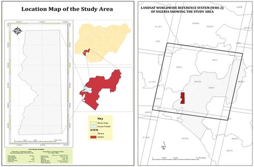
The study area is located on the north-western part of the Oluwa Forest, in Lisagbede Village, Odigbo LGA in Ondo State. Having an area of approximately 24,100 ha, it lies between 4°38′30″E, 6°43′50″N and 4°33′50″E, 6°59′8″N and is bounded in the north by the river Oni flowing into Oke-Igbo in Ondo State, in the south by Lagos – Benin expressway, the river Oluwa in the east and in the west by Omo Forest Reserve in Ogun state. The topography is between 137 m southward and 277 m towards the northern part of the forest and is gently undulating with a well-drained soil and outcrops of rocks of a basement complex of Precambrian era in some parts of the reserve (Omole & Akinwole, 2012). The rainfall pattern of the area is bimodal in nature and characterized with heavy downpour in September and October with annual rainfall ranging between 1500 and 2200 mm as reported by Onyekwelu, Mosandl, and Stimm (2006) and Omole and Akinwole (2012). The study area (path 190, row 055) on Landsat Worldwide Reference System (WRS-2) archive is shown in Figure 1.

Figure 1. Study area path and row on Landsat WRS-Ondo State Afforestation Project/(OSAP-OA1), Oluwa Forest, Ondo State, south-west Nigeria.

Field data

Sampling design

As recommended by Pouyat, Groffman, Yesilonis, and Hemandez (2002) and Okunade and Okunade (2007), to be in line with recommended practice, 10 random sample plots of 20 m × 20 m (from office-reconnaissance survey) were located in the field using a Garmin GPS. According to MacDicken (1997), the use of GPS receivers enables efficient and accurate placement of the plots. In each of the plots, all trees with DBH (i.e. diameter at 1.3m) exceeding 5 cm were measured with a 50 m tape and their heights measured with a distometer. For each plot, field sketch on the accessibility of the plot, the DBH and the heights of trees including the photograph of the plot were recorded. All field measurements were carried out in the month of March 2015.

Classification system

Tree major dominant tree-specie groups namely Tectona grandis, Gmelina arborea and indigenous species (such as Mahogany, Obeche and Opepe) were observed in the forest reserve. These were used as ground-truth parameters for the image classification as adopted by Abubakar et al. (2014). Trees were grouped in diameter classes as: sampling, i.e. younger tree class with DBH below 40 cm, the pole size tree with DBH ranging from 40 to 80 cm and the standard size trees with DBH above 80 cm. Smaller trees <5 cm DBH were not considered since they contribute a relatively small quantity of biomass (Brown, Gillespie, & Lugo, 1989). It is worthy of mentioning that replantation of T. grandis was carried out in the years 1989, 1986 and 1996 in some parts of the forest.

Soil sampling

Soil samples were randomly collected at the centre of each plot at depths of 0–15 and 15–30 cm, respectively, since the highest proportion of the total root is within the first 30 cm of the soil surface (Jackson et al., 1996; Bohm, 1979). About two-thirds of the carbon in terrestrial ecosystems comes from soil organic carbon (Eswaran, Van Den Berg, & Reich, 1993). As a result, the soil samples were carefully collected since it forms the major component of the result, thereby preventing the top-layer soil from falling to the lower samples according to best practices.

Data preparation

Estimation of biomass and carbon stock

AGB for the tree species strata was estimated from measured DBH and tree height using a generalized tree biomass regression equation for the specific precipitation zone (Brown, 1997):

where is the AGB in kg; DBH, diameter at breast height in cm; H is the height of tree in meter and this was converted to by multiplying with 0.001.

The regression equation of Brown et al. (1989) and Brown (1997) with = 0.97 was adopted. The criteria for using this model are that the trees parameter has a DBH > 5 cm, the study area is in the moist tropical forest with a rainfall pattern in the range 1500 < rainfall < 4000 mm. This study area is located in the moist tropical forest and has an annual rainfall range of 1700 to 2200 mm (Onyekwelu et al., 2006).

In summary, the total AGB of trees per sampled plots was multiplied by the number of trees per plot. Then, the biomass from all sampled plots per class was added to represent the biomass for each class (Table 1).

Table 1. Biomass area estimates.

Year	Forest stand	Gmelina arborea	Natural forest	Tectona grandis	Total
1984	Area (Ha)	2479	16,207	3012	21,698
	Biomass (ton)	56,574	369,852	68,738	495,164
1991	Area (Ha)	9162	8455	5371	22,988
	Biomass (ton)	209,073	192,949	122,584	524,606
2002	Area (Ha)	10,939	5949	6578	23,466
	Biomass (ton)	249,621	135,751	150,112	535,484
2010	Area (Ha)	4935	7406	11,652	23,993
	Biomass (ton)	112,620	168,997	265,903	547,520
2015	Area (Ha)	116	13,955	5,783	19,854
	Biomass (ton)	2649	318,456	131,977	453,082

Land cover area estimation was obtained from the supervised classification of Landsat imagery of 2015 using field observations as training classes for spectral signatures which were subsequently used for upscaling the biomass from plot to the entire land cover types.

Above ground biomass

The AGB, for each of the forest strata was estimated from the regression equation (Brown, 1997) using field measurements of DBH and height of individual trees that make up each stratum of the forest.

The AGB for the entire stand was then multiplied by the land cover area estimation.

(1)

Below ground biomass

BGB is estimated from AGB.  According to Ponce-Hernandez, (2004)  a non-destructive approach depends on belowground biomass values for vegetation as 20% of the aboveground biomass.

i.e.

(2)

Soil carbon stock.

The total organic carbon (TOC) of soil matter was determined by collecting soil samples from the sub-plot within the main sample plots (Table 13) using the Walkley–Black method (Pe´rie´ and Ouimet, 2008). A total of 20 samples at 0–15 and 15–30 cm were collected and for TOC (%Carbon). Soil carbon stock was computed by multiplying the concentration of total C by bulk density and the corresponding depth at which the sampling was done.

According to Kauffman and Donato (2012):

(3)

Carbon stock estimation

The sum total of all the biomass obtained from the three pools considered which are AGB, BGB and SOC was calculated and the carbon stock was obtained using Equation (4). According to Ponce-Hernandez (2004), total carbon stock can be calculated from

(4)

Image processing

Five Landsat scenes were acquired on 11 December 1984, 5 January 1991, 3 January 2002, 11 December 2010 and 15 January 2015 (path/row: 190/55) from the US Geological Survey (USGS) Earth Explorer website.

LULC change

In ERDAS Imagine 2014 software, a false colour composite (band 754) of the downloaded Landsat imagery (1984, 1991, 2002, 2010 and 2015) was carried out. The false colour composite enables vegetation to be detected readily on the imagery. The area of interest was defined and the training sites for the supervised classification extracted using the maximum likelihood algorithm. The imageries acquired were of the same season, which was between December and January. The ground-truth data (see the section “Field data”) was also incorporated as criteria for change detection. In line with Anderson, Hardy, Roach, and Witmer (1976) classification scheme, the study area was categorized into six classes for the classification based on spectral responses of the ground-truth features. The signature separability showing the statistical distance between signatures which determines how distinct the spectral signatures of features are to one another was also done. An accuracy assessment was, however, carried out for the classification (Tables 2 and 3). From the results of the supervised classification, post-classification change differencing technique described by Lu, Mausel, Brondízio, and Moran (2004) and Mas (1999) was used in assessing changes in land use/land cover within the study area.

Table 2. Accuracy totals.

Class name	Reference total	Classified total	Number correct	Producers accuracy	Users accuracy
Unclassified	0	0	0	–	–
Mountain patch	1	2	1	100.00%	50.00%
Water	0	0	0	–	–
Bare ground	2	1	1	50.00%	100.00%
Built up	0	0	0	–	–
Gmelina arborea	11	4	4	36.36 %	100.00 %
Deforested	15	15	13	86.67%	86.67%
Tectona grandis	27	25	25	92.59%	100.00%
Natural forest	64	73	63	98.44%	86.30%
Total	120	120	107

Table 3. Conditional kappa.

Class name	Kappa
Unclassified	0
Mountain patch	0.4958
Water	0
Bare ground	1
Built-up	0
Gmelina arborea	1
Deforested	0.8476
Tectona grandis	1
Natural forest	0.7065

Accuracy assessment

The overall accuracy for the 2015 classification was obtained as 89.17%, while the overall kappa coefficient was 0.8223. The accuracy totals for the same year are shown in Table 2, while the corresponding conditional kappa for each of the categories is shown in Table 3.

Normalized Difference Vegetation Index)

The surface reflectance imagery was downloaded from USGS webpage (http://espa.cr.usgs.gov) by placing an order for each of the surface reflectance data of the imagery used except for 2002 and 2010 which were not available. The NDVI was carried out using both the top of atmosphere (TOA) reflectance from the raw Landsat imagery and that from the surface reflectance in order to compare both the results.

Geospatial database for monitoring carbon content

The biomass distribution map of 2015 (as a reference biomass regime for other years) was done in ArcMap 10.1 (Figure 14) using the inverse distance weight interpolation technique in the Spatial Analyst tools from the ground-truth (sample plots) measurements as adopted by Abubakar et al. (2014). However, to monitor the biomass distributions and carbon contents over the years, NDVI of the Landsat imageries of 1984, 1991, 2002, 2010 and 2015 was used as explained by Klemas and Pieterse (2015), that AGB is usually evaluated using one of several vegetation indices. The most common index used is the NDVI, which is the ratio of the difference between the Red and Near Infrared reflectance and their sum. NDVI indicates how healthy the leaves are and can be related to plant biomass and also its carbon content.

Results

Tree height-DBH

The height and DBH of the trees measured are shown in Table 4.

Table 4. Aggregate of height and diameter-at-breast height field measurements.

Forest stand	Height (m)	DBH (cm)	No. of trees	Remarks
Plot 1: Tectona grandis	20.53	182	39	Planted in 1989
Plot 2: Gmelina aborea	17.64	127	81	Not available
Plot 3: Tectona grandis	23.71	167	78	Planted in 1986
Plot 4: Tectona grandis	17.28	84	78	Planted in 1996
Plot 5: Natural forest	16.37	337	208	Natural plantation
Plot 6: Tectona grandis	16.91	140	22	Not available
Plot 7: Tectona grandis	15.72	86	30	Heavily degraded
Plot 8: Tectona grandis	22.30	80	84	Slowly harvested
Plot 9: Gmelina aborea	32.45	86	136	Not available
Plot 10: Tectona grandis	23.62	115	42	Not available
Total			760

Soil organic content

The result of the soil organic content derived from TOC analysis using the Walkley–Black method is shown in Tables 5 and 6.

Table 5. Forest stand composition showing its frequencies by height class.

		Frequency by height class (H in m)
20 m × 20 m	Forest stand	2–4	4–6	6–8	8–10	10–12	12–14	14–16	16–18	18–20	Total
Plot 1	Tectona grandis	0	8	0	0	0	0	31	0	0	39
Plot 2	Gmelina arborea	34	0	0	0	0	0	47	0	0	81
Plot 3	Tectona grandis	0	12	0	0	0	0	0	0	28	40
Plot 4	Tectona grandis	62	0	0	0	0	16	0	0	0	78
Plot 5	Natural forest	0	185	0	0	0	23	0	0	0	208
Plot 6	Tectona grandis	0	10	0	0	12	0	0	0	0	22
Plot 7	Degraded Forest	0	0	3	27	0	0	0	0	0	30
Plot 8	Tectona grandis	0	0	65	0	0	0	19	0	0	84
Plot 9	Gmelina arborea	0	0	0	0	0	0	88	48	0	136
Plot 10	Tectona grandis	0	0	5	0	0	0	0	37	0	42
Total		96	215	73	27	12	39	185	85	28	760
Mean		9.6	21.5	7.3	2.7	1.2	3.9	18.5	8.5	2.8	76
Height per hectare		240.0	537.5	182.5	67.5	30.0	97.5	462.5	212.5	70.0	1900

Table 6. Forest stand composition showing its frequencies by DBH size class.

		Frequency by size class (DBH in cm)
20 m × 20 m	Forest stand	0–20	20–40	40–60	60–80	80–100	100–120	>120	Total
Plot 1	Tectona grandis	0	0	8	0	0	0	31	39
Plot 2	Gmelina arborea	0	0	34	47	0	0	0	81
Plot 3	Tectona grandis	0	12	0	0	0	28	0	40
Plot 4	Tectona grandis	0	62	16	0	0	0	0	78
Plot 5	Natural forest	0	0	0	0	185	0	23	208
Plot 6	Tectona grandis	0	10	0	0	0	12	0	22
Plot 7	Degraded forest	0	3	27	0	0	0	0	30
Plot 8	Tectona grandis	0	65	19	0	0	0	0	84
Plot 9	Gmelina arborea	88	0	0	48	0	0	0	136
Plot 10	Tectona grandis	0	5	0	0	37	0	0	42
Total		88	157	104	95	222	40	54	760
Mean		8.8	15.7	10.4	9.5	22.2	4.0	5.4	76.0
DBH per hectare		220.0	392.5	260.0	237.5	555.0	100.0	135.0	1900.0

Tables 3 and 4 show the soil organic carbon at different soil horizon and the proportion of soil organic carbon in the forest stand, respectively, with the degraded forest having 46.7% of the entire SOC, while the natural forest has 6.7%, which is the lowest organic carbon content in soil.

Table 5 shows that T. grandis has the overall highest biomass of 101,016.92 ton/ha followed by the natural forest with 90,743.729 ton/ha then 3240.115 ton/ha for degraded forest and 396.647ton/ha for G. arborea which has the lowest total biomass.

Field-based measurements

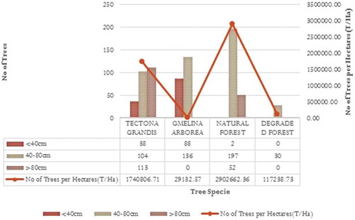
About 760 trees measured had their DBH between 13 and 245 cm. The DBH was categorized into classes similar to that adopted by Abubakar et al. (2014). Figure 2 shows the distribution of the tree stand density with T. grandis having trees within the sapling, pole and standard sizes, while G. arborea has between sapling and pole sizes. The natural forest has between pole and the largest standard sizes with the degraded forest only within pole sizes.

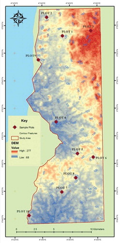
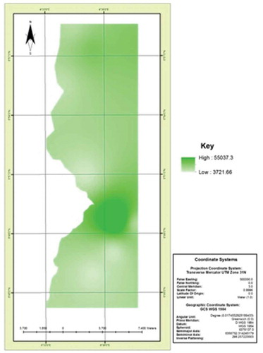
Figure 2. Digital Elevation Model showing the location of the sample plots.

Allometric equation

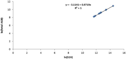
The allometric equation of Brown (1997) was applied to field measurements to estimate the AGB for the sample plots. The equation was found to exhibit a positive correlation of as shown in Figure 3.

Figure 3. Allometric regression equation on field measurements.

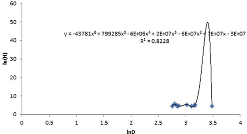
Figure 4 shows a high logarithmic relationship and not a linear relationship between AGB and the product of the square of DBH and height (D²H).

Figure 4. Logarithmic relationship between height and DBH.

Other allometric equations from field measurements relationships

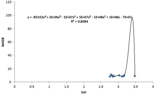
Figures 4 and 5 show the relationships between the logarithmic functions of height, DBH and AGB. A positive correlation of for lnH – lnDBH graph and for lnAGB – lnH graph was found.

Figure 5. Logarithmic relationship between aboveground biomass and height.

Other strong relationships which exist between field-measured height and diameter are polynomial in nature.

It was established from the field measurement that height is strongly correlated with the AGB, having .

Total AGB

The AGB from all the forest stands (T. grandis, G. arborea, indigenous species and degraded forest) was added to represent the biomass for the entire forest.

Total BGB

The BGB is estimated from AGB as 20% of the AGB (see the section “Below ground biomass”).

Soil carbon

The organic carbon of soil samples collected at 0–15 and 15–30 cm depth was determined by multiplying the concentration of total C by bulk density and the corresponding depth at which the sampling was done.

The Bulk density was determined from the unit weight and volume of the soil sample.

The soil carbon from the top/surface soil (0 cm) to depth of 15 cm was added to the soil carbon up to 30 cm. The total soil carbon was then added for the all the forest stands.

Total carbon stock

The total carbon stock was estimated as the total stock of carbon in the ecosystem, including above ground and below ground stock. The constituents of the below ground stock are the carbon content in roots and all BGB and the carbon in the soil.

The total below ground carbon stock is the addition of both carbon in forest floors and litters and those beneath the soil.

(5)

The above ground carbon stock was used as 50% of the AGB for converting forest AGB to carbon stock (IPCC, 2003; Ponce-Hernandez, 2004).

The total carbon stock for the study area was estimated as the summation of the total above ground carbon stock and the total below ground carbon stock.

(6)

Carbon dioxide (CO₂) sequestered

The total carbon stock can be converted to by multiplying carbon stock by 3.67 which is the ratio of the molecular weights between and carbon (Kauffman & Donato, 2012).

(7)

The total carbon sequestered by the forest reserve is estimated to be 359 megaton of carbon.

LULC change

Tables 2 and 3 show the accuracy assessment result, and the LULC changes are illustrated in Tables 7–10, and Table 14 including Figure 6.

Figure 6. The distribution of sampled trees in OSAP OA1 (sapling, pole and standard classes).

Biomass map

Figure 3 shows the biomass distribution map of the study area obtained from ground-based plot-level measurement as used by Goswami, Verma, and Kaushal (2014) and Abubakar et al. (2014) for the current biomass variation.

Normalized Difference Vegetation Index

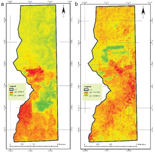
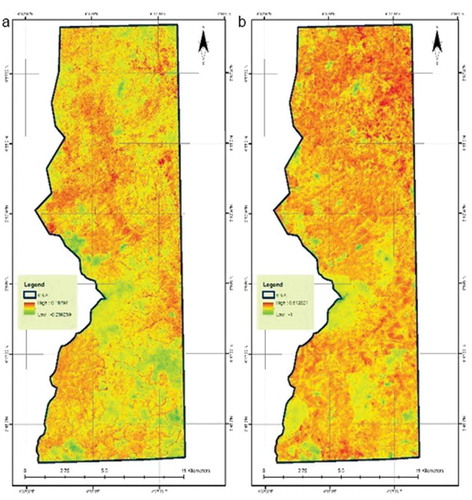
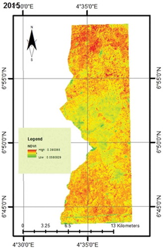
The NDVI for the years 1984–2015 using the digital numbers directly from the imagery is shown in Figures 7–9. The years 1984 and 1991 have NDVI values which range from 0.377 to 0.345, indicating a reduction in biomass while in 1991 and 2002, there was an increase from 0.345 to 0.408; and between 2002 and 2010 an increase from 0.408 to 0.513 was observed. However, between 2010 and 2015 a huge decrease from 0.513 to 0.360 was observed when compared to the trends observed from 1984 to 2010.

Figure 7. (a) NDVI for 1984 (using top of atmosphere (TOA) reflectance). (b) NDVI for 1991 (using top of atmosphere (TOA) reflectance).

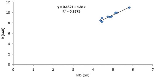
Figure 8. (a) NDVI for 2002 (using top of atmosphere (TOA) reflectance). (b) NDVI for 2010 (using top of atmosphere (TOA) reflectance).

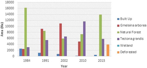
Figure 9. NDVI for 2015 (using top of atmosphere (TOA) reflectance).

It was observed that the NDVI for the years 1984–1991 using surface reflectance varied between 0.278–0.570 and −0.120 to 0.083 compared to using the TOA reflectance (digital number) which varied between 0.084–0.377 and 0.055–0.345 (Figures 7 and 10), indicating an increase in biomass as confirmed by the LULC change. While, the NDVI values using the digital numbers for 2015 range between 0.058 and 0.390 compared to 2015 NDVI values from surface reflectance between −0.174 and 0.141 (Figures 9 and 10), which is still in the theoretical range of −1 to 1 for NDVI. This shows that the NDVI was not affected by the surface reflectance in the study area, which although compensates for the adverse effects of the atmosphere from clouds, atmospheric aerosol, gases, etc. However, this was further proved by carrying out the NDVI for the entire Landsat scene, which was in the range of −1 to 1 as shown in Figure 10.

Figure 10. Landsat-derived NDVI (using surface reflectance).

Predicting biomass and carbon content

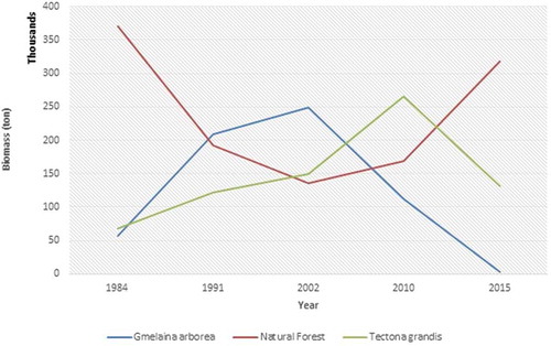
The biomass database trend extracted from the three vegetative land cover (natural forest, G. arborea and T. grandis) shows the variation from 1984 to 2015. G. arborea and T. grandis give a decrease in biomass and in turn carbon content from 2002 and 2010, respectively; while, the afforested species are steadily replaced by the natural forest as illustrated in Figure 11.

Figure 11. Biomass estimates between 1984 and 2015.

Tables 1 and 11 show the biomass estimates and database obtained using the forest stands of 2015 field measurements as reference on the imageries for the various epochs. Land cover area for each of the forest stand was multiplied by the stands plot measurement biomass per unit area.

Table 7. Land use land cover area.

	1984	1991	2002	2010	2015
Land use land cover	Area (Ha)	Area (Ha)	Area (Ha)	Area (Ha)	Area (Ha)
Built-up	2500.035	1207.990	740.028	186.964	432.878
Gmelina arborea	2479.137	9161.847	10,938.711	4935.161	116.066
Natural forest	16,207.351	8455.265	5948.792	7405.639	13,955.108
Tectona grandis	3012.196	5371.798	6578.097	11,652.176	5783.411
Wetland	–	–	–	15.998	450.000
Deforested	–	–	–	–	3,908.475
Grand total	24,198.718	24,196.900	24,205.628	24,195.938	24,195.983

Table 8. Land use land cover change in area.

	1984–1991	1991–2002	2002–2010	2010–2015
Land use/land cover	Change	Change	Change	Change
Built-up	−12.92	4.68	−5.53	2.46
Gmelina arborea	66.83	17.77	−60.04	−48.19
Natural forest	−77.52	−25.06	14.57	65.49
Tectona grandis	23.60	12.06	50.74	−58.69
Wetland	–	–	0.16	−0.16
Deforested	–	–	–	39.08

Table 9. Land use land cover percentage.

	1984	1991	2002	2010	2015
Land use land cover	% Cover	% Cover	% Cover	% Cover	% Cover
Built-up	10.33	4.99	3.06	0.77	1.79
Gmelina arborea	10.24	37.86	45.19	20.40	0.48
Natural forest	66.98	34.94	24.58	30.61	57.68
Tectona grandis	12.45	22.20	27.18	48.16	23.90
Wetland	–	–	–	0.07	0.00
Deforested	–	–	–	–	16.15
Grand total	100.00	100.00	100.00	100.00	100.00

Table 10. Land use rate of change.

	1984–1991	1991–2002	2002–2010	2010–2015
Land use/land cover	Rate	Rate	Rate	Rate
Built-up	−51.68%	−38.74%	−74.74%	131.53%
Gmelina arborea	269.56%	19.39%	−54.88%	−97.65%
Natural forest	−47.83%	−29.64%	24.49%	88.44%
Tectona grandis	78.33%	22.46%	77.14%	−50.37%
Wetland		–	0.07%	−99.72%
Deforested		–	–	16.15%

Table 11. Plot biomass database estimate of 2015.

Plot	Easting (mE)	Point (mN)	H (m)	lnH	D (cm)	lnD	n	lnD2H	AGB (ton)	TOC%	BGB (ton)	Above ground carbon	Below ground carbon	Total carbon (ton)	Total CO2 (ton)
Plot1	675,803.250	768,972.850	20.531	3.022	182.000	5.204	39	13.430	20.712	16	4.142	10.356	20.142	30.499	111.929
Plot2	673,696.230	771,454.960	17.640	2.870	127.000	4.844	81	12.559	8.880	16	1.776	4.434	17.774	22.216	81.533
Plot3	679,595.720	769,653.050	23.708	3.166	167.000	5.118	78	13.402	20.153	14	4.031	10.077	18.031	28.107	103.153
Plot4	674,967.180	757,490.460	17.278	2.849	84.000	4.431	78	11.711	3.897	14	0.779	1.948	14.779	16.728	61.391
Plot5	677,823.030	753,258.570	16.370	2.795	337.000	5.820	208	14.436	55.043	14	11.009	27.522	25.009	52.530	192.786
Plot6	679,929.360	752,786.530	16.911	2.828	140.000	4.942	22	12.711	10.301	16	2.060	5.150	18.060	23.211	85.182
Plot7	675,727.910	748,120.670	15.720	2.755	86.000	4.454	30	11.664	3.721	15	0.744	1.861	15.744	17.605	64.610
Plot8	677,594.190	750,021.410	22.300	3.105	80.000	4.382	84	11.869	4.542	15	0.908	2.271	15.908	18.179	66.717
Plot9	672,578.310	765,758.730	32.453	3.480	86.000	4.454	136	12.388	7.527	9	1.505	3.764	10.505	14.269	52.367
Plot10	671,360.210	744,972.300	23.615	3.162	115.000	4.745	42	12.652	9.722	14	1.944	4.861	15.944	20.805	76.355

Discussion

To estimate the AGB and BGB in the study area, determine the total carbon content and evaluate the carbon dioxide () sequestered, a total of 760 trees were measured on field. The DBH of all the trees measured ranges from 26 to 130 cm. The smallest tree category by size (DBH) was below 40 cm having an average stand density of 612.5 DBH/ha, the next in size is the pole size trees with the DBH ranging from 40 to 80 cm having an average stand density of 497.5 DBH/ha and the standard tree with the DBH greater than 80 cm having an average tree stand density of 790 DBH/ha as shown in Tables 4 and 5. The natural forest has the highest number of trees of 208 also with the biggest DBH of 197 and 52 cm standard size and pole size categories, respectively, due to its diversity in tree species. Ebuy, Lokombe, Ponette, Sonwa, and Picard (2011) explained the difficulty in estimating heterogeneous or mixed-species forest stand, hence the reason for adopting (Brown, 1997) pan-topical allometric model which gave a positive correlation of 1 between the field measurements and the biomass. We observed a linear relationship between the logarithmic functions of the DBH and AGB with R² = 0.9375 (Figure 12), while the relationship between DBH and height is non-linear (Figure 4). As stated earlier, DBH had a stronger correlation with biomass compared to the tree heights, which agrees with both Brown et al. (1989) and Chave et al. (2004). Odiwe et al. (2012) also used the Brown et al. (1989) allometric model in estimating the carbon stock in topsoil, standing floor litter and AGB in T. grandis plantation 10 years after establishment in Ile-Ife, south-western Nigeria.

Figure 12. Logarithmic relationship between aboveground biomass and DBH.

Degraded forest (originally T. grandis plantation) was found to have the highest soil organic carbon of 46.7%. The total AGB for the study area (163 Mg ton/ha) shown in Table 12 was smaller compared with (Brown et al., 1989) assertion that AGB for undisturbed tropical forests of Asia and the world to be an average of 215 and 192 Mg/ha, respectively. The total aboveground carbon stock estimated was 81 Mg tons of carbon, while the total belowground carbon stock was 16 Mg tons of carbon with soil carbon of 5.797 tons (see the sections “Soil carbon” and “Total carbon stock”).

Table 12. Percentage of soil organic carbon for the forest stands.

Soil organic carbon
Plot	Forest stand	0-15 cm	15-30 cm	Total (cm)	Percentage (%)
1	Tectona grandis	31.91	38.29	70.20	33.126
2	Gmelina arborea	15.25	13.44	28.69	13.538
3	Degraded forest	6.60	8.21	98.89	46.664
4	Natural forest	7.79	6.35	14.14	6.672
	Total			211.92	100

Table 13. Soil total organic content (TOC) at different soil depths.

Soil-TOC (%)
Plot	Forest stand	0-15 cm	15-30 cm
1	Tectona grandis	6.5	9.61
2	Gmelina arborea	7.1	8.48
3	Tectona grandis	7.04	6.68
4	Tectona grandis	5.17	8.48
5	Natural forest	7.79	6.35
6	Tectona grandis	7.39	8.96
7	Tectona grandis-degraded	6.6	8.21
8	Tectona grandis	5.91	9.49
9	Gmelina arborea	2.64	6.77
10	Tectona grandis	6.4	7.39

Table 14. Total aboveground and belowground biomass estimates.

Forest stand	Total aboveground biomass (ton)	Total belowground biomass (ton)	Total biomass (ton)
Tectona grandis	84,178	16,839	101,017
Gmelina arborea	330.521	66.126	396.647
Natural forest	75,619	15,125	90,744
Degraded forest	2700	540.381	3240
Total	162,826	32,571	195,397

A total of 359 Mg ton/ha of CO₂ was estimated to have been sequestered in the area. This value, though considering varying area extent, is higher compared to the values of carbon stock recorded in Ile-Ife (28.18 ton/ha) and in other regions of Africa reported by Odiwe et al. (2012) that the cocoa agroforestry in South Cameroon has 152 Mg ton/ha, while oil palm and rubber plantations in Cameroun both have 66–88 and 248–264 Mg ton/ha, respectively. Based on the 2015 supervised classification, the area extent of land use is in the order of natural forest > T. grandis > degraded forest > G. arborea of 13,955.108, 5783.411, 3908.475 and 116.066 ha, respectively.

In assessing the rate of change in LULC between 1984 and 2015, a decrease of 1292 Ha, a rate of 51.68% and 7752 Ha at the rate of 47.83% in bare-ground /built-up area and natural forest, respectively, was observed between 1984 and 1991. Contrarily, both G. arborea and T. grandis increased in area by 6683 Ha at the rate of 269.56% and 2360 Ha at the rate of 78.33%.

Between 1991 and 2002, the area of both built-up and natural forest further reduced by 468 Ha at 38.74% and 2506 Ha at 29.64%. However, G. arborea and T. grandis increased by 1777 Ha at the rate of 19.39% and 1206 Ha at the rate of 22.46%, respectively.

However, between 2002 and 2010, G. arborea began its areal reduction to 4935 Ha in 2010 compared to 10,939 Ha observed in 2002, a rate of 54.88%. As a result of this, there was a corresponding expanse in the area covered by the natural forest. It increased by 24.49%, from the 5949 Ha observed in 2002 to 7406 Ha in 2010. At the same time, the decrease in the built-up area/bare ground persisted with 187 Ha observed in 2010, compared to the 740 Ha observed in 2002. There was on the other hand an increase in T. grandis. Its area cover at this time was observed to be 11,652 Ha, a further increase of 77.14%. The drastic reduction of the G. arborea could be as a result of the heavy and indiscriminate logging activities.

Similarly, between 2010 and 2015, G. arborea experienced a further reduction of 97.65% whereas T. grandis reduced by 50.37%. Whereas, the built-up area/bare ground increased by 131.53%, while the natural forest further increased by 88.44%. It is evident from the last 5 years under consideration that the rate at which the forest was degraded is quite alarming. This may be due to the World Bank withdrawing its support from the afforestation project in 1998, thus ending any reforestation or planting efforts. In addition, by this time, the presence of dead trees and logged woods in several places coupled with the non-stop entries of lumber vehicles into the forest and their exits from it is an evidence of disproportionate exploitation of these timbers (USAID, 2008). Afterwards, this setback made the forest a means of revenue for the Ondo State Government.

Finally, in order to develop a geospatial database for monitoring carbon content in the study area, NDVI (Figure 15) was used in estimating biomass and the biomass graphical pattern which shows the vegetation cover in Figure 13, and both T. grandis and G. arborea show a steady decline in biomass from 2002 to 2015. We can clearly deduce that, if factors such as deforestation are not controlled, the CS capability of the study area may continue to reduce. (Ponce-Hernandez (2004), Yin, Udelhoven, Fensholt, Pflugmacher, and Hostert (2012) and Klemas and Pieterse (2015) explained that the use of band ratio indices such as NDVI exploits the discriminating power of the infrared band ratios of chlorophyll activity in vegetation; however, the strength in the relationships may vary with tree structure and state of health of the vegetation and other environmental parameters.

Figure 13. Land use land cover between 1984 and 2015.

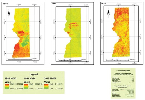
Figure 14. Biomass distribution map.

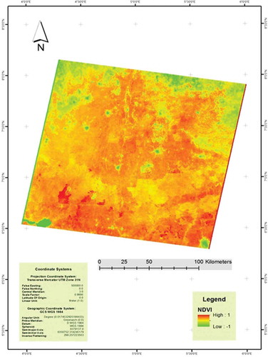
Figure 15. Landsat-derived NDVI (from digital numbers) for the entire scene (path 190/row 55).

Conclusion

It can be concluded that forests help maintain conditions that make life possible, from regional hydrological cycles to global climate changes and that the existence of deforestation, degradation and poor forest management practices has been proved in the study area. This research has been able to estimate a total of of AGB, BGB, total carbon stock of and of carbon dioxide sequestered by the study area. Also, change in LULC carried out between 1984 and 2015, which was confirmed by the NDVI, revealed that the forest is drastically losing its greenness and carbon storage capacity to uncontrolled logging and forest degradation.

Furthermore, the deforestation, degradation and poor forest management practices have been proved in the study area. The Oluwa Forest might be one of the tropical rainforests projected by Urquhart, Walter, David, & Chris (2007), to disappear within the next 100 years. In mitigating against this, both constant field data as well as remote sensing data should be deployed in assessing the carbon sequestered by the study area, since, to our knowledge, this may be the first CS project in Ondo State Afforestation Project (OSAP-OA1), Oluwa Forest which supports other researches advocacy on the need to carry out more biomass estimation and CS projects in Africa especially, since the continent is a huge consuming one and fast developing, thus the consequences of our anthropogenic activities should be scientifically assessed.

Acknowledgement

Our sincere appreciation goes to the Management of the Ondo State Afforestation Project for the support extended to us, which ensured the successful execution of this project.

Disclosure statement

No potential conflict of interest was reported by the authors.

References

- Abubakar, A., Abdulkadir, A., Jibrin, A., & Abubakar, R.B. (2014). An appraisal of forest degradation and carbon sequestration of Effan Forest Reserve in Kwara State. Global Journal of Science Frontier Research: H Environment & Earth Science, 14, 3.
- Ahmedin, A.M., Bam, S., Siraj, K.T., & Solomon Raju, A.J. (2013). Assessment of biomass and carbon sequestration potentials of standing Pongamia pinnata in Andhra University, Visakhapatnam, India. Bioscience Discovery, 4(2), 143–148.
- Anderson, J.R., Hardy, E.E., Roach, J.T., & Witmer, R.E. (1976). A land use and land cover classification system for use with remote sensor data (pp. 28). Washington, D.C.: U.S. Government Printing Office.
- Bajracharya, S. (2008). Community carbon forestry: Remote sensing of forest carbon and forest degradation in Nepal. Enschede: ITC.
- Banskota, K., Karky, B.S., & Skutsch, M. (2007). Reducing carbon emission through community managed forests in the Himalaya. International Centre for Integrated Mountain Development (ICIMOD), Norwegian Agency for Development Cooperation (NORAD).
- Bohm, W. (1979). Methods of studying roots systems. Ecological studies no. 33. Berlin, Germany and New York, USA, Springer-Verlag. In BP, 2004: Statistical review of world energy.
- Brown, S. (1997). Estimating biomass and biomass change of tropical forests: A primer. A forest resources assessment publication. FAO Forestry Paper 134, Rome. 17(203), 177–186.
- Brown, S.A.J., Gillespie, J.R., & Lugo, A.E. (1989). Biomass estimation methods for tropical forests with application to forest inventory data. Forest Sciences, 35(4), 881–902.
- Chave, J., Condit, R., Aguilar, S., Hernandez, A., Lao, S., & Perez, R. (2004). Error propagation and scaling for tropical forest biomass estimates. Philosophical Transactions of the Royal Society B: Biological Sciences, 359(1443), 409–420.
- Cienciala, E., Seufert, G., Blujdea, V., Grassi, G., & Exnerová, Z. (2010). Harmonized methods for assessing carbon sequestration in European Forests European Commission Joint Research Centre Institute for Environment and Sustainability (pp. 3–328). Luxembourg: Publications Office of the European Union.
- Cortés, G., Girotto, M., & Margulis, S.A. (2014). Analysis of sub-pixel snow and ice extent over the extratropical Andes using spectral unmixing of historical Landsat imagery. Remote Sensing of Environment, 141, 64–78. doi:10.1016/j.rse.2013.10.023
- Ebuy, J., Lokombe, J.P., Ponette, Q., Sonwa, D., & Picard, N. (2011). Allometric equation for predicting aboveground biomass of three tree species. Journal of Tropical Forest Science, 23(2), 125–132.
- Eswaran, H., Van Den Berg, E., & Reich, P. (1993). Organic carbon in soils of the world. Contribution from world soil resources, USDA Soil conservation. Soil Science Society of America journal, 57, 192–194.
- Gibbs, H.K., Ruesch, A.S., Achard, F., Clayton, M.K., Holmgren, P., Ramankutty, N., & Foley, J.A. (2010). Tropical forests were the primary sources of new agricultural land in the 1980s and 1990s. Proceedings of the National Academy of Sciences, 107, 16732–16737. doi:10.1073/pnas.0910275107
- Goswami, S., Verma, K.S., & Kaushal, R. (2014). Biomass and carbon sequestration in different agroforestry systems of a Western Himalayan watershed, Biological Agriculture and Horticulture. An International Journal for Sustainable Production Systems, 30(2), 88–96.
- Haghparast, H., Delbari, A., & Kulkarni, D.K. (2013). Carbon sequestration in Pune university campus with special reference to geographical information system (GIS). Department of Environmental sciences, Pune University, India & BAIF Development Research Foundation, Pune, India. Annals of Biological Research, 4(4), 169–175.
- Houghton, R.A. (2005). Aboveground forest biomass and the global carbon balance. Global Change Biology, 11, 945–958.
- IPCC. (2001, October 05). Climate change 2001 report. Retrieved from: http://www.grida.no/publications/other/ipcc_tar/?src=/climate/ipcc_tar/wg1/099.htm
- IPCC. (2003). Good practice guidance for land use, land use change and forestry. Geneva: Intergovernmental Panel on Climate Change (IPCC.
- Jackson, R.B., Canadell, J., Ehleringer, J.R., Mooney, H.A., Sala, O.E., & Schulze, E.D. (1996). A global analysis of root distributions for terrestrial biomes. Oecologia, 108, 389–411. doi:10.1007/BF00333714
- Jeyanny, V., Balasundram, S.K., & Husni, M.H.A. (2011). Geo-spatial technologies for carbon sequestration monitoring and management. American Journal of Environmental Sciences, 7(5), 456–462. doi:10.3844/ajessp.2011.456.462
- Kauffman, J.B., & Donato, D.C. (2012). Protocols for the measurement, monitoring and reporting of structure, biomass and carbon stocks in mangrove forests. Working Paper 86. CIFOR, Bogor, Indonesia.
- Klemas, V., & Pieterse, A. (2015). Using remote sensing to map and monitor water resources in arid and semiarid regions. In: T. Younos, T.E. Parece (Eds.), Advances in Watershed Science and Assessment, The Handbook of Environmental Chemistry (p. 33). Springer International Publishing Switzerland. DOI 10.1007/978-3-319-14212-8_2
- Lu, D., Mausel, P., Brondízio, E., & Moran, E. (2004). Change detection techniques. International Journal of Remote Sensing, 25, 2365. doi:10.1080/0143116031000139863
- MacDicken, K.G. (1997). A guide to monitoring carbon storage in forestry and agroforestry projects. USA: Winrock International Institute for Agricultural Development.
- Mas, J.F. (1999). Monitoring land-cover change: A comparison of change detection techniques. Presented at the Fourth International Conference on Remote sensing for Marine and Coastal Environments, Orlando, Florida. Taylor and Francis Ltd. doi:10.1080/014311699213659
- Momodu, A.S., Siyanbola, W.O., Pelemo, D.A., Obioh, I.B., & Adesina, F.A. (2011). Carbon flow pattern in the forest zones of Nigeria as influenced by land use change. African Journal of Environmental Science and Technology., 5(9), 700–709.
- Nowak, D.J., Greenfield, E.J., Hoehn, R.E., & Lapoint, E. (2013). Carbon storage and sequestration by trees in urban and community areas of the United States. Environmental Pollution, 178, 229–236. doi:10.1016/j.envpol.2013.03.019
- Odiwe, A.I., Rofiat, A.A., & Ogunsanwo, O. (2012). Carbon stock in topsoil, standing floor litter and above ground biomass in Tectona grandis plantation 10-years after establishment in Ile-Ife, southwestern Nigeria. International Journal of Biological and Chemical Sciences, 6(6), 3006–3016.
- Okunade, I.O., & Okunade, K.A. (2007). Towards standardization of sampling methodology for evaluation of soil pollution in Nigeria. Journal of Applied Sciences and Environmental Management, 11(3), 81–85.
- Omole, A.O., & Akinwole, A.O. (2012). Assessment of technical compliances to landowners guides in forest roads of Oluwa Forest Reserve, Ondo State Nigeria. Nigerian Journal of Agriculture, Food and Environment, 8(2), 41–44.
- Onyekwelu, J.C., Mosandl, R., & Stimm, B. (2006). Productivity, site evaluation and state of nutrition of Gmelina arborea plantations in Oluwa and Omo forest reserves, Nigeria. Forest Ecology and Management, 229, 214–227. doi:10.1016/j.foreco.2006.04.002
- Pe´Rie,´, C., & Ouimet, R. (2008). Organic carbon, organic matter and bulk density relationships in boreal forest soils. Canadian Journal of Soil Science, 88(3), 315–325. doi:10.4141/CJSS06008
- Ponce-Hernandez, R. (2004). Assessing carbon stocks and modelling win–win scenarios of carbon sequestration through land-use changes. ROME: Food and agriculture organization of the united nations.
- Pouyat, R., Groffman, P., Yesilonis, I., & Hemandez, L. (2002). Soil carbon pools and fluxes in urban ecosystem. Environmental Pollution, 116, 107–118. doi:10.1016/S0269-7491(01)00263-9
- Urquhart, G., Walter, C., David, S., & Chris, B. (2007). Tropical deforestation. NASA earth observatory library: Tropical deforestation fact sheet. Retrieved from http://earthobservatory.nasa.gov/Features/Deforestation/
- USAID. (2008). Nigerian biodiversity and tropical forestry assessment. Maximizing agricultural revenue in key enterprises for targeted sites (Markets). Retrieved from https://www.google.com/urlsa=t&rct=j&q=&esrc=s&source=web&cd=1&cad=rja&uact=8&ved=0ahUKEwjMvY2Q187UAhWFCcAKHbhXBXwQFggsMAA&url=http%3A%2F%2Fpdf.usaid.gov%2Fpdf_docs%2FPnadn536.pdf&usg=AFQjCNFA25bOrM_0heNVD3SvSQSm6AtgTw&sig2=A8ssyjeyxmfPSvWdtNO_Aw
- Van Beek, C.L. (2010). Environmental Science and Policy, 13, 89–96. doi:10.1016/j.envsci.2009.11.001
- Vashum, K.T., & Jayakumar, S. (2012). Methods to estimate above-ground biomass and carbon stock in natural forests – A review. Journal of Ecosystem & Ecography, 2, 116. doi:10.4172/2157-7625.1000116
- Yin, H., Udelhoven, T., Fensholt, R., Pflugmacher, D., & Hostert, P. (2012). How Normalized Difference Vegetation Index (NDVI) trends from Advanced Very High Resolution Radiometer (AVHRR) and Système Probatoire d’Observation de la Terre VEGETATION (SPOT VGT) time series differ in agricultural areas: An Inner Mongolian Case Study, 4(11), 3364–3389.