Improvements of storm surge forecasting in the Gulf of Venice exploiting the potential of satellite data: the ESA DUE eSurge-Venice project

ABSTRACT

The northern Adriatic Sea is affected by storm surges, which often cause the flooding in Venice and the surrounding areas. We present the results of the eSurge-Venice project, funded by the European Space Agency (ESA) in the framework of its Data User Element programme: the project was aimed to demonstrate the potential of satellite data in improving storm surge forecasting, with focus on the Gulf of Venice. The satellite data used were scatterometer wind and altimeter sea level height. Hindcast experiments were conducted to assess the sensitivity of a storm surge model to a model wind forcing modified with scatterometer data and to altimeter retrievals assimilated with a dual 4D-Var system. The modified model wind forcing alone was responsible for a reduction of the mean difference between modelled and observed maximum surge peaks from −15.1 to −8.2 cm, while combining together scatterometer and altimeter data the mean difference further reduced to −6.0 cm. In terms of percent, the improvements in the reduction on the mean differences between modelled and observed surge peaks reaches 46% using only the scatterometer data, and 60% using both scatterometer and altimeter data.

KEYWORDS:

• Storm surge
• scatterometry
• ocean winds
• altimetry
• data assimilation
• Adriatic Sea
• Venice

Introduction

Storm surges are intense risings of the sea level, caused by severe meteorological conditions. They can be extremely destructive in proximity of low-lying coastal areas, as when the surge makes landfall, extensive flooding may occur. In more extreme cases, the surge may lead to loss of life and significant economic losses. In the Mediterranean Sea, the most relevant storm surges occur in the Adriatic Sea (Figure 1), more frequently from autumn to spring, usually associated to sirocco, a steady, moist and warm south-easterly wind. Sirocco is tunnelled by the orography contouring the basin and pushes the water toward the Gulf of Venice (Franco, Jectic, Rizzoli, Michelato, & Orlíc, 1982). Often sirocco lasts for days, moving notable amounts of water in the Gulf of Venice. In the past decades, an increase in the frequency and intensity of flooding events has been registered in the city of Venice, in the northern Adriatic Sea (Figure 1).

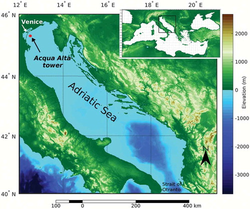
Figure 1. Adriatic Sea, its position in the Mediterranean Sea (inset), the surrounding orography, the bathymetry of the basin and the position of the Venice City (top left).

The prevention of risks and damages associated to important surge events is usually achieved with the aid of storm surge numerical models. For this reason, the city of Venice has used and developed such systems since the 1970s (Canestrelli & Pastore, 2000). For practical applications, the prediction of the surge level field in such a basin can be decomposed in two contributions: the first is the initial condition of the surge; the second is the dynamical evolution of the surge caused by the meteorological forcing, namely sea level pressure and wind. Other contributions, like the wave set-up, non-linear interactions between storm surge, astronomical tide and waves, baroclinic forces and river discharges, are generally negligible and can be quantified as less than 2 cm (Lionello, Sanna, Elvini, & Mufato, 2006). The accuracy of the storm surge prediction is thus strongly constrained by those of the atmospheric forcing and of the initial sea level field from which the dynamical evolution of the surge develops: a better knowledge of both would increase the accuracy of the storm surge forecast itself (Cavaleri et al., 2010; Peng, Xie, & Pietrafesa, 2007; Wilson, Horsburgh, Williams, Flowerdew, & Zanna, 2013). This goal was achieved in the framework of the eSurge-Venice project – a project funded by the Data User Element programme of the European Space Agency (ESA) – by using satellite scatterometer wind and radar altimetry Total Water Level Envelope (TWLE: a quantity easily derived from the sea level anomaly) observations to increase the reliability and accuracy of the storm surge prediction in the Gulf of Venice. Satellite-borne scatterometer winds were used to mitigate the biases between the model and the measured winds with a methodology named wind-bias mitigation (Zecchetto, Della Valle, & De Biasio, 2015). Satellite altimetry brought instead a significant improvement of the sea level background field across the basin, through the assimilation of TWLE retrievals into the storm surge model (SSM) SHYFEM (online: http://www.ismar.cnr.it/shyfem), with a dual 4D-Var assimilation algorithm.

The following sections present the results of the experiments made during the eSurge-Venice project: firstly a brief characterization of the storm surge in the Adriatic Sea is given. Then, the satellite and model data used in this work are presented, followed by the description of the SSM employed for the hindcast experiments as well as of the methodologies conceived to bring the satellite data into the SSM. A rapid sketch of the experimental set-up is given before the closing section dedicated to discussion and conclusions.

In De Biasio et al. (2016), we summarized the results of the eSurge-Venice project. With that work we intended to reach a broad audience more interested in storm surge studies than in the methods used to achieve those results. In the present article, we focus to a well-targeted audience (remote sensing) more interested on the synergistic use of models and altimetry- and scatterometry-based observations.

Storm surges in the Adriatic Sea

The Adriatic Sea is deeper in its southern part and shallower in the North. It has an elongated shape and is surrounded by mountain chains (see Figure 1): these characteristics favour the occurrence of intense storm surge events (SEVs) in the northern (closed) end, in particular during autumn and winter and with higher elevations than in the rest of the Mediterranean Sea. In the Adriatic Sea, the astronomical tide has semi-diurnal characteristics, with almost diurnal behaviour during neap-tides. In the Gulf of Venice, the higher amplitudes are those of the M₂, K₁ and S₂ components (24.7, 15.9 and 13.9 cm, respectively; adapted for the year 2017 (Centro Previsioni e Segnalazioni Maree, 2017), while all the other have amplitudes lower than 6 cm. The harmonic superposition of the main eight tide components (M₂, S₂, N₂, K₂, K₁, O₁, P₁ and S₁) determines a maximal amplitude of the astronomical tides of ~40 cm, which contributes to the total sea level with storm surge, seiches and other minor components. Typical storm surge elevations in the Gulf of Venice (northern Adriatic Sea) range from few centimetres to few tens of centimetres, but can occasionally reach much higher elevations in very particular circumstances, as the 1966 flooding of Venice, during which the maximum peak registered was of 170 cm (De Zolt, Lionello, Nuhu, & Tomasin, 2006).

Well-known meteorological conditions are responsible for the occurrence of storm surges in the Adriatic Sea: a low-pressure system situated west of the Adriatic Sea causes the sirocco blowing along the basin’s major axis (Lionello et al., 2012). The sirocco, associated with the crossing of cyclones over the Mediterranean Sea, is effective in pushing the water towards the northern closed end of the Adriatic Sea. Often in the southern and central parts of the basin blows the sirocco, while in the northern basin the wind comes from north-east (bora). The Adriatic Sea morphology favours also the set-up of free oscillations of the basin water, called seiches. They occur as a response to unstable conditions like a horizontal gradient in the water level due to the wind action, for example, when a steady and strong sirocco wind suddenly changes to bora in the northern Adriatic Sea (Leder and Orlić, 2004). Their period is essentially determined by the bathymetry and the dimensions of the basin. The two major seiches in the Adriatic Sea have periods of 21.2 and 10.8 h. The former is the principal one in the basin, propagates along its main dimension and is characterized by a period close to the diurnal tides. The latter propagates counterclockwise and has a period similar to the semi-diurnal tides. Seiches of lower amplitudes and periods are also observed. On average, seiches produce level displacement of 20–30 cm but can reach 60–80 cm and are progressively attenuated in 10–15 days. Having a period close to those of the diurnal and semi-diurnal tide components, the two principal seiches can produce high water levels even days after a SEV, when in phase with the astronomical tide.

Satellite and model data

The scatterometer wind data

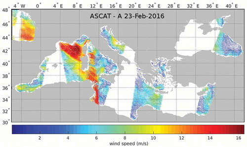
Scatterometers are satellite-borne radar instruments able to determine both the intensity and direction of the wind at the sea surface, also known as Ocean Wind Vector (OWV). The scatterometer wind data used in this work are the NASA QuikSCAT version 3 L2B OWV (Jet Propulsion Laboratory, 2013a), the EUMETSAT ASCAT-A L2 OWV, ASCAT-A L2 Coastal OWV, ASCAT-B L2 Coastal OWV (Eumetsat Ocean and Sea Ice Satellite Application Facility, 2012) and Oceansat-2 L2B OWV (JPL, 2013b), all at 12.5 km × 12.5 km of sample resolution cell. Scatterometer winds, which are referenced to equivalent neutral air-sea stability conditions, have been adjusted to real stability conditions using the boundary layer model described in (Liu, Katsaros, & Businger, 1979). The parameters needed to calculate these adjustments are the mean sea level pressure, the air and dew temperatures at 2 m, derived from the global model analyses of the European Centre for Medium-Range Weather Forecasts (ECMWF), Reading, UK (Klinker et al., 2000), and the sea surface temperature (SST) from satellite observations. An example of a typical 1-day spatial coverage of the ASCAT scatterometer onboard the EUMETSAT Metop-A satellite (ASCAT-A), over the Mediterranean Sea, is reported in Figure 2: both ascending and descending swaths are visible, but the complete coverage of the sea is not achieved by ASCAT-A alone. ASCAT-B (not shown) was put in an orbit slightly shifted in time and space, providing enough data for an almost complete daily coverage of the Mediterranean Sea by the two ASCAT sensors.

Figure 2. ASCAT-A scatterometer ascending and descending swaths over the Mediterranean Area. Typical spatial coverage pattern for a whole day (2016–02-23).

The ECMWF model data

The atmospheric model fields used in the hindcast experiments are the analysis fields of the ECMWF global model at different resolutions (at 40, 25 and 16 km of equivalent grid, depending on the SEV date, as the model resolution increased from 40 to 25 km in 2006, and to 16 km in 2010) interpolated on a 0.125° regular grid. These were the wind components at 10 m of height from the sea surface and at real air-sea stability conditions, and the mean sea level pressure, provided in the analysis at synoptic hours (00, 06, 12, 18 UTC). The ECMWF mean sea level pressure, air temperature at 2 m and dew temperature at 2 m analysis fields have also been used to adjust the scatterometer wind from neutral to real stability conditions.

Temporal match-up and spatial collocation of scatterometer observations and atmospheric model data

The scatterometer data have been interpolated on the same 0.125° regular grid used for ECMWF data, with a Laplacian method which does not change the statistics of the wind speed and direction. The ECMWF model data have been linearly interpolated to the scatterometer overpass times (Accadia, Zecchetto, Lavagnini, & Speranza, 2007).

The altimeter data

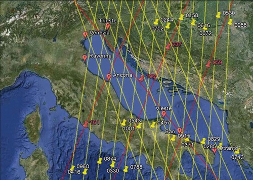
The altimeter is a radar aboard a satellite that measures the distance of the sea surface from the instrument. We used altimetry data coming from three different sensors: POSEIDON-2 on NASA/CNES Jason-1 (2002–2009), POSEIDON-3 on NASA/CNES/NOAA/EUMETSAT Jason-2 (2008-present) and RA-2 on ESA Envisat (2002–2010). The tracks over the Adriatic Sea cyclically re-visited by the three satellites are shown in Figure 3.

Figure 3. Ground track coverage in the Adriatic Sea. Red lines: expected crossing by Jason-1 and Jason-2. Yellow lines: expected crossing by Envisat.

Altimeter standard products have reduced accuracy in coastal areas and regional seas. This is the case of the Adriatic Sea, which can be considered almost entirely a coastal sea (Zecchetto, De Biasio, & Accadia, 2012). For this reason, reprocessed products dedicated to the monitoring of coastal areas have been adopted. Those supplied by CTOH (Center for Topographic studies of the Ocean and Hydrosphere) (Roblou, Lyard, Le Hénaff, & Maraldi, 2007) have been found the most suitable among others coastal altimetry products (COASTALT, PISTACH). The altimetry parameter of interest for the present hindcast experiments is the TWLE*, the level reached by the water under the effects of the ocean dynamics and the atmospheric forcing. It is derived from the sea surface height corrected for the atmospheric delays, the sea state bias, the loading tides and the solid earth tides, but with the local response to atmospheric forcing (inverse barometer and high-frequency) left in (Cipollini, Scarrott, & Snaith, 2014). TWLE* has a strict connection to the sea surface height anomaly in the standard altimetry products, as in the latter both the tides and the atmospheric forcing are usually stripped out, while in TWLE* only the oceanic tides are subtracted. It corresponds to the TWLE with the astronomical tide removed.

In-situ data

The SSM time series of surge level were compared against the sea level observations registered by the tide gauge of the Acqua Alta oceanographic platform (45° 18.51ʹ N; 012° 30.30ʹ E), situated about 15 km off-shore the Italian coast (red dot in Figure 1). The astronomical tide signal was removed from hourly sea level observations with harmonic analysis. The in-situ data are monitored and quality-controlled by the storm surge Warning Authority of Venice.

The storm surge model

The SHYFEM model (Umgiesser, Melaku Canu, Cucco, & Solidoro, 2004) is based on the finite element discretization technique, with a semi-implicit time stepping. In order to avoid mass conservation issues, it uses a scattered grid. For the present application the equations included the Coriolis, the hydrostatic terms, the horizontal turbulent diffusion, the bottom friction and the wind and pressure forcing terms, while baroclinic terms and tidal forcing were not included. In fact, the baroclinic terms have a much longer time scale than that typical of storm surge. Consequently, their contribution, in the operational context, is often accounted for by the mean level of the water in the previous day(s). The tide contribution, given the low interaction with the other components in the Adriatic Sea (Bajo and Umgiesser, 2010), can be left out from the model formulation, and considered as an independent field. The equations are vertically integrated, in a two-dimensional hydrostatic shallow water formulation. The simulations run over a computational grid of the Mediterranean Sea. The grid was finer in the shallow zones and in the Adriatic Sea, while it was coarser in the central sub-basins. Open boundary conditions were assumed in the Atlantic Ocean border. The simulations were forced with surface wind and pressure from the ECMWF analysis, and the computed level was properly identified with the meteorological surge.

Use of satellite data in the storm surge model simulation

In the following sections, we present the two applications of satellite data developed to bring the potential of satellite data in support to storm surge modelling.

Bias mitigation of the atmospheric model wind forcing

Small basins surrounded by significant orography are areas where the atmospheric modelling performance is lower than in open-ocean. In the Adriatic Sea, for example, the scatterometer-model wind bias has been found particularly dependent on time and space (Zecchetto & Accadia, 2014). Such bias enters in the storm surge modelling and reduces the accuracy of the predicted surge. A solution would be to use scatterometer winds instead of atmospheric modelling winds in SS modelling. The scatterometer winds, however, are not suitable to be used directly as forcing in the SSMs because of the irregular spatial and temporal sampling. On the other hand, assimilation of scatterometer winds into atmospheric models is already done in several global (and regional) models. Unfortunately, the thinning applied to scatterometer data (50–100 km) in order to avoid model instabilities prevents the scatterometer wealth of details to be fully exploited in regional seas. Nonetheless, scatterometer observations can be useful in quantifying the observations-model bias, a parameter that can be beneficial in reducing the bias itself. Preliminary investigations of differences and similarities between scatterometer and model winds have been carried out (Zecchetto & Accadia, 2014; Zecchetto et al., 2012) by means of the normalized wind speed bias Δw^N(i,j), defined in Equation 1, where w(i,j) is the wind speed at the location (i,j) of a grid covering the Adriatic Sea, the symbol <…> indicates the temporal average of the quantity in brackets and the superscripts sc and e refer to scatterometer and atmospheric model, respectively. The wind direction bias Δθ(i,j), where θ(i,j) is the wind direction, is the mean difference between the scatterometer and the model wind direction, and is defined in Equation 2.

(1)

(2)

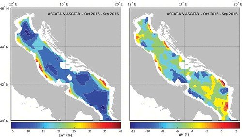
The representation of the statistics of the two bias over a period of one year (October 2015–September 2016) is reported in Figure 4: the left panel shows the normalized wind speed bias between the two data sets, always positive (ECMWF underestimates winds with respect to scatterometer), reaching more than 35% along some of the coasts. The mean bias of the wind direction, in the right panel, is less dramatic, showing differences in the range [−12 + 2] degrees, indicating that ECMWF winds are slightly rotated clockwise with respect to scatterometer observations.

Figure 4. Scatterometer-ECMWF wind speed normalized bias (left) and wind direction bias (right) for one year of data (Octorber 2015 to September 2016). The scatterometers considered are ASCAT-A and ASCAT-B.

The mitigation of the two bias in the model fields uses the bias registered in the preceding few days between scatterometer observations and model analyses, introducing them as counteracting terms in the definition of the mitigated model wind. This methodology has been first proposed and investigated in Zecchetto et al., 2015). The approach for the wind speed relies on the normalized bias Δw^N(i,j) (Equation 3) as counteracting term, while that for the wind direction simply relies on Δθ(i,j) (Eq. 2), i.e.:

(3)

(4)

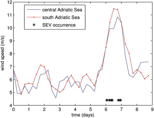
where the prime symbol marks the bias-mitigated variables. From the operational point of view, the normalized wind speed bias and the wind direction bias, calculated beforehand over a running observation window of the previous three days, are applied to determine the (mitigated) model wind fields of the day following the observation window. The mitigation procedure was applied to the analyses of every day of the SSM simulations. The hindcast experiments have been thus conducted performing storm surge simulations with the standard (reference) analysis fields in order to obtain a SSM control set, and the mitigated analysis fields, in order to obtain the experimental SSM hindcast runs. From an operational point of view, if atmospheric forecasts had been used instead of analyses, this methodology would have allowed the use of the mitigated wind fields into the SSM for the simulations of the following 24 h before the midnight of each day, providing high-quality storm surge forecast for the following day, several hours in advance with respect to the expected surge peak. The statistical significance of the bias mitigation technique is ensured by a width of the observation window of around three days, as this is the mean duration of the sirocco wind in the Adriatic Sea before a SEV. A shorter window would have resulted in a less reliable scatterometer-model bias estimation, while enlarging arbitrarily the observation window would have turned to a loss in correlation between observations pertaining to different meteorological phenomena falling inside the window, and thus to a reduction of the statistical significance. In Figure 5 are shown the distributions of the wind speed aggregated in central and southern Adriatic Sea, for all the SEVs considered in this study. Wind speeds ≥7 m/s have been used as an indicator to determine the width of the observation window. The value of 3 days is evaluated as the mean duration of a SEV in the Adriatic Sea.

Figure 5. The mean duration of the sirocco wind during the storm surge events under consideration. The duration in the central Adriatic Sea (blue solid line) is shorter than in the southern Adriatic (red solid line). A 7 m/s wind speed is considered for the determination of the observation window width.

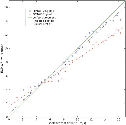
In order to show the improvements of the mitigated model wind over the original (reference) wind, the scatter-plot of the non-mitigated (original) and mitigated ECMWF atmospheric model wind speed data against scatterometer observations, for 8 SEVs, is reported in Figure 6. Scatterometer-model collocated data coming from three days are considered for each SEV: 2 days before the SEV and the SEV day itself. The best fit of the model wind data set is markedly moved towards the perfect agreement line by the mitigation procedure.

Figure 6. Scatterplot of the ECMWF atmospheric model wind speed and scatterometer wind speed. Reference (original) model data are in red. Bias-mitigated model data in blue. Dashed lines correspond to the best fits. Green solid line represents the perfect agreement. Data have been aggregated in 0.5 m/s bins before calculating the fit lines.

Altimeter data assimilation

Altimeter records have much more variance than SSM simulations and cannot be directly assimilated into the SHYFEM SSM. A pre-processing non-linear fit of the TWLE* retrievals was thus performed in order to obtain smoother altimeter spatial signals, with a characteristic length scale near to the actual spatial resolution of the SSM. The differences between this signal and the modelled surge were assimilated, after subtracting the minimum distance between the two signals, with a dual 4D-Var algorithm (Courtier, 1997). This technique was used with the aim of supplying a more realistic initial state of the modelled sea state at the beginning of the hindcast run, in substitution of that supplied by the spin-up phase.

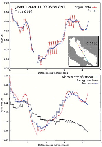
In Figure 7 the Jason-1 altimeter TWLE* and SSM profiles along the altimeter track #0196 on 9 November, 2004, 03:34 GMT, are shown. The left panel shows the original TWLE* retrievals (in red), and the pre-processing fit needed to reduce variability (in blue) for the assimilation in the SHYFEM SSM. In the right panel are reported the TWLE* fit again (in red), the SHYFEM surge background state profile along the J-1 track before assimilation (in black), and the SHYFEM surge analysis state profile along the J-1 track after assimilation (in blue). The impressive convergence of the analysis state after assimilation is evident, given the very different initial signals (SHYFEM background and altimeter TWLE*). The case shown here is one of the most lucky: the assimilation cycle in other SEVs did not perform so well, partly because of a low number of TWLE* retrievals. The inset in the left panel shows the position of the J-1 track #0196 in the Adriatic Sea. Only the altimeter tracks crossing the Adriatic Sea the day before the SEV have been assimilated: as a matter of fact, the scarcity of altimeter passes in the (very narrow basin of the) Adriatic Sea made the assimilation impracticable in four SEV cases.

Figure 7. The Jason-1 altimeter track #0196 profile over the Adriatic Sea, on 9 November, 2004, 03:34 GMT. Left panel: the original TWLE* data (red), and the fit needed to reduce variability (blue). Right panel: The TWLE* fit (red), the SHYFEM surge background state profile along the J-1 track before assimilation (black), and the SHYFEM surge analysis state profile along the J-1 track after assimilation (blue). The inset in the left panel shows the position of the J-1 track #0196 in the Adriatic Sea.

Storm surge hindcast experiments set-up

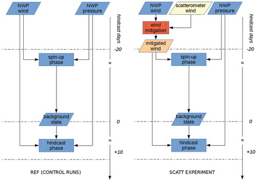
The experiments have been carried out on 22 SEVs from 2004 to 2012. First of all, for each SEV a control run was performed using the standard procedure: a numerical simulation starting 20 days before the SEV occurrence, in order to avoid model spin-up issues, and finished 10 days after. Each run is divided in two phases: a spin-up phase to reach the hydrodynamic equilibrium, and a hindcast phase. The beginning of the hindcast phase is set at 00 UTC the day before each SEV. The simulations in the data set obtained with the standard procedure are referred to as REF runs henceforth, and represent the control runs against which the experiment runs have been compared. No satellite data were ingested during the REF control runs. The REF simulations are the reference forecasts from which the performance of the hindcast experiments has been evaluated. A schematic diagram of the data flow and the modelling processes involved in the realization of the REF (control) runs is shown in the left panel of Figure 8: the atmospheric (Numerical Weather Prediction: NWP) model wind and pressure are fed to the SSM during the spin-up phase, terminating with a background state of the surge. The hindcast phase starts from the background and is driven again by model wind and pressure.

Figure 8. Left: schematic flow chart of REF (control runs) simulations. Right: schematic flow chart of the SCATT hindcast experiment simulations. Scatterometer data are ingested during the SCATT experiment.

Three other hindcast experiments have been performed, and the corresponding simulation sets are marked with the labels SCATT, ALT and SCATTALT. They were designed to test the sensitivity of the SSM to the introduction of satellite data:

1. the SCATT experiment was performed substituting the standard ECMWF model wind forcing with the fields modified by the mitigation procedure with the scatterometer observations. This experiment was conducted on 22 SEVs. Only scatterometer data were used in the simulations of the SCATT data set. A schematic diagram of the data flow is shown in the right panel of Figure 8: the NWP wind undergoes the mitigation procedure before being fed to the spin-up and the hindcast phases;

2. the ALT hindcast experiment was designed to test the impact of altimetry into the SSM through assimilation of the TWLE* retrievals. It was performed on 18 SEVs. Only altimeter data were used in this experiment with the aim of improving the background surge level field of the first day of the SEV, and the schematic data flow is presented in the left panel of Figure 9: the outcome of the spin-up phase, the surge background state, is changed by the assimilation cycle into a new surge state called analysis state, which is used as starting point in the hindcast phase;

   Figure 9. Left: schematic flow chart of ALT hindcast experiment simulations. Right: schematic flow chart of the SCATTALT hindcast experiment simulations. Altimeter data are ingested during the ALT experiment, while both altimeter and scatterometer data are ingested during the SCATTALT experiment.

   

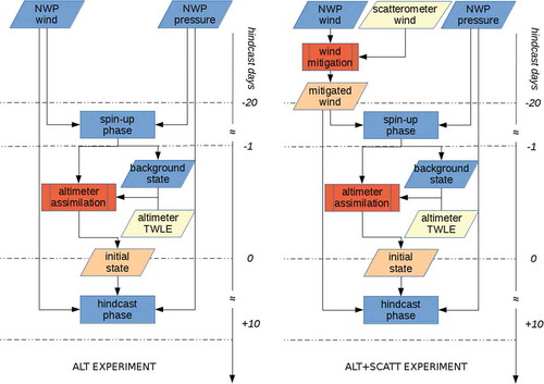
3. the SCATTALT hindcast experiment was set-up to assess the possible interaction between the mitigation technique and the assimilation procedure when applied together, and to quantify the performance of the SSM using both scatterometer-mitigated NWP winds and altimeter TWLE* retrievals. This experiment was conducted on 18 SEVs. Both altimeter and scatterometer data have been ingested in the SCATTALT hindcast experiment, as shown in the right panel of Figure 9.

To summarize, in the four simulation sets, the wind bias mitigation procedure (performed with satellite scatterometer wind data) and the assimilation of TWLE* (derived from satellite altimeter retrievals) were organized as follows:

• (1) REF (control) simulations: wind bias mit.: NO TWLE* assimilation: NO;

• (2) SCATT simulations: wind bias mit.: YES TWLE* assimilation: NO;

• (3) ALT simulations: wind bias mit.: NO TWLE* assimilation: YES;

• (4) SCATTALT simulations: wind bias mit.: YES TWLE* assimilation: YES.

The wind bias mitigation (abbreviated “mit.” in the list above) and the TWLE* assimilation impact on the SSM simulations in different ways. While the wind bias mitigation technique modifies all the model wind forcing fields, thus acting at the boundaries of the simulation throughout the whole period of its evolution, the assimilation of altimeter TWLE* take place only once, during the day before the SEV occurrence, and improves the background state at the beginning of the SEV day, thus acting on the initial conditions of a single day of simulation. The improved background is the analysis state. It is thus expected that the two satellite-data ingestion procedures do not interfere with each other, although they have a reciprocal impact which cannot be completely avoided.

The hindcast experiments have been carried out for 22 SEVs from 2004 to 2012 (see Table 1). Four SEVs had no TWLE* records in the assimilation time window. For them, only the wind bias mitigation impact has been assessed.

Table 1. Dates, times, levels and altimeter data availability of the SEVs used for the hindcast runs. Levels in cm.

Date (yyyy/mm/dd)	Time UTC	Total level	Astronomical level	Surge level	Altimeter assimilation
2004/10/31	08	116	57	59	X
2004/11/10	06	121	65	56	X
2004/12/26	08	112	62	50	X
2005/12/03	08	119	64	55	X
2008/12/01	06	127	42	85	X
2008/12/10	06	114	68	46	X
2009/01/26	22	110	59	51	X
2009/02/02	23	110	40	70	X
2009/03/29	20	114	51	63	X
2009/11/30	06	118	66	52	X
2009/12/19	08	115	49	66	X
2009/12/22	02	114	46	68	X
2010/01/07	01	116	60	56	X
2010/02/28	20	113	68	45	X
2010/11/10	10	110	56	54	X
2010/11/19	07	115	69	46	X
2010/11/26	09	110	44	66
2011/02/16	20	113	65	48	X
2012/10/27	05	110	37	73
2012/10/31	20	121	22	99
2012/11/11	05	118	49	69	X
2012/11/28	19	116	14	102

The model-derived sea surface level field of the day before the SEV, at the end of the spin-up phase, was used as background state for the hindcast phase in all the simulations. The improvements of the SSM performance in the different configurations were assessed comparing the modelled surge level of the control and the experiment runs against the in-situ hourly sea level observations at the Acqua Alta platform, located in the northern Adriatic Sea, 15 km off-shore the Venice coast, where good quality tide gauge data were available. The tidal signal was removed from observations by means of harmonic analysis. The observed surge was compared directly to the modelled surge after a correction of the mean sea level. The beginning of the simulated time series was set through a lagged-correlation analysis: the simulated values were shifted over a range of ±6 h centred on the corresponding observed maximum surge peak, and the lag was chosen as that maximizing the correlation of the time series of the following 36 hourly values of observed and simulated surge. The correlation model chosen in this context, as well as for the analysis of the simulations results, is linear, also known as the Pearson’s product-moment coefficient. It is the covariance of two variables divided by the product of their standard deviations. The lag distributions resulted centred around a negative value of 1.5 h, with the 93% of the values within the interval [−3, +1] h. The lag distributions of the SCATT, ALT and SCATTALT experiments were almost similar to that of the REF control runs, with little (≤1 h) differences of the mean lag.

Results

The results of the experiments were analysed in terms of the linear correlation coefficients between the time series of the 36-hourly modelled and observed surge values, of their bias, of their centred (unbiased) RMS difference, of the difference of the modelled and observed maximum peak elevation (skew error, ε_s) and of the relative skew error (ε_s/observed surge peak). The values of the statistical parameters averaged over the SEVs for the four experiments are reported in Table 2.

Table 2. Summary results of the hindcast experiments.

	REF	SCATT	ALT	SCATTALT
Linear correlation <r>	0.889	0.890	0.890	0.894
Skew error <εs> (cm)	−15.1	−8.2	−11.5	−6.0
Relative skew error <εs/max surge level> (%)	−15.9	−8.2	−12.2	−5.9
Bias <b> (cm)	−5.7	−3.1	−6.0	−3.5
Centred RMS difference <cRMSd> (cm)	6.8	6.5	6.7	6.4

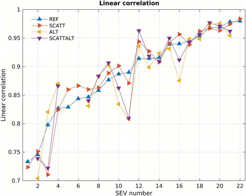
The Pearson’s correlation maintained very high and almost constant over all the experiment runs (Figure 10) confirming that the methodologies conceived for the ingestion of satellite data into the SSM were very well tolerated by the surge model, and did not alter significantly the correlation of the hindcast time series with respect to the control runs. Some experiment simulations performed signally worse than REF in few cases: ALT (SEV # 2, 10, 11 and 16); SCATTALT (SEV # 3 and 11); SCATT (SEV # 3). In total, we found lower performances in 9% of the experiments simulations. It is easily recognized that SEV # 3 poor results in SCATT and SCATTALT experiments are due to a low performance of the bias mitigation procedure (scatterometer data are common to both SCATT and SCATTALT experiments), while for SEV # 11 the cause has to be imputed to the altimeter assimilation (altimeter data are common to both ALT and SCATTALT experiments). For all the other SEVs, the correlation coefficients were very close to the REF results.

Figure 10. Pearson’s linear correlation coefficient of the observed and modelled surge time series for all the SEV, ordered by increasing values of the REF control runs. The results of the REF experiments are in blue. The others experiments are SCATT (orange), ALT (yellow) and SCATTALT (purple).

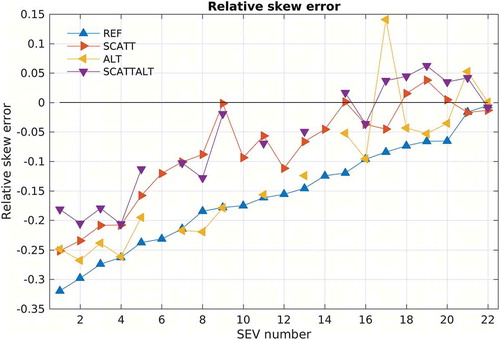
The drop in absolute magnitude of the relative skew error ε_s from the control runs to the experiments was rather impressive. The control runs mean was −15 cm, while the SCATTALT runs mean (best experimental result) was as low as −6 cm, with only one SEV whose ε_s resulted worse than that of the corresponding control run. As for the ALT experiment, in three SEVs, ε_s was slightly worse than the corresponding REF runs, while the SCATT runs were always better or similar to the REFs. In Figure 11 we have reported the relative skew error (ε_s/observed surge at peak) of the 22 SEVs in all the experiments. The black solid line divides the graph in two regions: below it the simulations underestimating the observed surge peak, above it the simulations overestimating it. The positive impact of satellite data on the representation of the surge peak is evident, as the vast majority of the hindcast simulations are placed between the REF runs curve (blue) and the zero line. The percent values of the hindcast runs are almost always smaller than that of the REF runs. For the last few SEVs to the right of Figure 11, the relative skew error is not as good as the preceding SEVs, but it is also the region where differences between in-situ data and simulations were very little when compared to the observed surges, and thus marginal.

Figure 11. Skew errors of the modelled and observed surge peaks for all the SEV, relative to the observed surge (ε_s/obs). The results of the REF experiments are in blue. The others experiments are SCATT (orange), ALT (yellow) and SCATTALT (purple). Data are ordered with increasing value of the relative skew error of the REF runs. The black solid line marks the zero of skew error: data below the line correspond to underestimation of the observed surge peak.

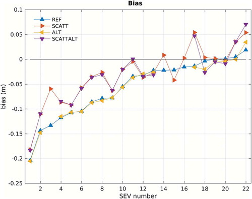
The horizontal black line in Figure 12, which shows the bias between modelled and observed surge time-series of all the experiments, marks the regions of model underestimation (negative bias) and overestimation (positive bias). The absolute magnitude of the mean bias was deeply reduced in the experiments using the mitigation procedure (SCATT and SCATTALT ~3 cm) laying between the zero-line and the REF and ALT curves. On the other hand, REF and ALT experiments, those without wind bias mitigation (see Table 2), show very similar behaviours and a much larger bias (~−6 cm). This result is in agreement with the conjecture that the main ability of the wind bias mitigation procedure is to reduce the global bias of the model wind. Figure 12 shows the values of the bias for each SEV and experiment: the REF and ALT runs have about the same bias in each SEV; so do SCATT and SCATTALT runs, which also have similar relative skew errors, but show smaller bias in the majority of the SEVs, with respect to REF and ALT.

Figure 12. Bias of the modelled and observed surge time series for all the SEV, ordered by increasing values of the REF control runs: REF (blue), SCATT (orange), ALT (yellow) and SCATTALT (purple). The black solid line marks the zero bias: data below the line correspond to underestimation of the observed surge.

The statistical values of the reference simulations (REF runs) are in blue in Figures 10, 11 and 12. The REF runs of the 22 SEVs were obtained using the standard analysis fields of the ECMWM global model as forcing in the SHYFEM SSM. The general trend is the underestimation of the observed surges (Figure 11), with relative skew errors ranging from few percent to 30% with a rather uniform distribution of the values. In very few cases, the other three experiments gave worse results than the reference. In the SCATT experiment, the values of the relative skew error (in orange in Figure 11) are in general smaller than those of the REF runs (in blue). In the SCATT and SCATTALT experiments, only 7 SEVs showed a relative skew error outside the boundaries of ±10%, which is a remarkable result when compared to the REF simulations that performed outside those limits in 15 cases. The relative skew errors for the ALT experiment are plotted in yellow in Figure 11. The assimilation of the altimeter TWLE* into the hydrodynamic model does not seem to bring results as relevant as those obtained in the SCATT experiment. Nevertheless, the skew error slightly improves from −15.1 cm to −11.5 cm, indicating a modest but evident impact of TWLE* assimilation in the SSM. In the SCATTALT experiment (purple triangle marks), the impact of the assimilation adds to the that of the wind mitigation, determining a further reduction of the relative skew error and bias absolute magnitudes with respect to the already good results of the SCATT experiment, while maintaining very similar values of linear correlation. Of course, the main improvements are brought by the mitigated wind forcing.

Discussion and conclusions

The simulations with the wind correction (SCATT) show a pretty uniform performance. The real wind is almost always underestimated in the Adriatic Sea in case of an extreme event, and this type of correction does not alter in general the phase of the surge (see discussion about lagged correlation), but increases the amplitude of the modelled surge peaks. In the 22 cases considered, it never worsened the forecast. The best simulation set is that with both the corrections (SCATTALT), even though, in some cases, the simulations with just the wind correction (SCATT) are slightly better. This happens when the altimeter data have low quality or even when the scatterometer increases too much the surge, since the two contributions, SCATT and ALT, have the tendency to add up. Moreover, between the REF and the SCATT simulations, a higher level of covariance has been observed than between the REF and the altimeter-based ones (ALT and SCATTALT), as in the altimeter-based simulations sometimes the assimilation introduces abrupt changes of the surge level in the time domain. The simulations with altimeter assimilation (ALT and SCATTALT) sometimes show a time shift of the surge curve and a more radical change of its shape, adding artefacts around the assimilation window time (not shown).

The wind bias mitigation methodology takes the scatterometer wind as the reference to adjust the ECMWF forecast winds. This is a requirement given by the general underestimation of ECMWF winds in the Mediterranean Sea (Zecchetto & De Biasio, 2007). The characteristics of these biases do not seem to be peculiar to the ECMWF global model, but are exhibited also by other atmospheric models (De Biasio, Miglietta, & Zecchetto, 2014). A relatively small part of the bias is possibly ascribed to the scatterometers themselves: in the present work we have used QuikSCAT, Oceansat-2, ASCAT-A and ASCAT-B data, and small biases are normal between different datasets. According to Bentamy, Grodsky, Carton, Croizé-Fillon, and Chapron (2012), the bias between the QuikSCAT and ASCAT-A data sets on a worldwide analysis is lower than 1 m/s, with several spatial differences. From an independent study conducted by us about the period of QuikSCAT and ASCAT-A overlapping (March to November 2009), the bias in the Mediterranean Sea resulted almost negligible (0.6 m/s). The biases of the other data sets have not been investigated and will form the object of forthcoming studies. The reliability of the method depends strictly from the number of scatterometer re-visit in the area of interest. Some periods during this study were characterized by the highest temporal sampling of the Adriatic, ≈2 swaths per day by QuikSCAT and, during the period when QuikSCAT and ASCAT-A flew together, ≈3 swaths per day. Two data per day is seen here as the minimum temporal sampling to get maps of ∆w^N and ∆θ with some statistical significance, also considering the time length of the SS occurrence.

Being the first attempt to assimilate altimeter data into a SSM, we believe that the results obtained in the ALT and SCATTALT hindcast experiments are very promising, even if the positive improvement brought by altimetry-based assimilation is lower than that provided by the scatterometer-based wind-bias mitigation. Apart from the complexity of the model assimilation set-up, other issues prevent the full exploitation of the method: first of all, only the altimeter tracks falling within the day before each SEV are assimilated. Those falling outside would require to enlarge the assimilation window. In this case, even though a higher number of data were available, the correction to the initial state would be too far from the event to have a significant influence. A rather interesting approach would be, instead, to extend the assimilation to the whole Mediterranean Sea, because this would significantly increase the number of tracks within the assimilation period. In this respect, the assimilation of tide gauge data together with altimeter TWLE* should further improve the impact of the method. Also, the sensitivity of the SSM to several assimilation cycles during the spin-up phase should be assessed: in so doing, one would possibly get to the end of the spin-up phase with a more realistic initial surge state (level and water transport) than that predicted by a single assimilation cycle, because the impact of the assimilation would be spread over a longer period starting backward in the past, with a larger number of observations. Unfortunately, even if other and more complex assimilation experiments become feasible, their impact at the operational level would remain limited, given the accuracy needed in this type of application (cm) and the consequent long delays for data distribution (weeks to months) with the present altimeter satellite. However, the situation is going to change soon for the better, as the new generation of ESA Sentinel-3 SAR altimeters will provide better coverage and shorter latencies (Donlon et al., 2012). Nonetheless, the impact in SSM of such a new type of altimetry data has not been assessed yet, and will be examined as soon as the data become available.

The hindcast experiments conducted have shown a remarkable impact of earth-observation data into SSM predictions. The synergy between the bias mitigation and the altimeter assimilation in the reduction of the error may be probably ascribed to the different sources of error they act on, which are the forcing wind at the model boundaries and the surge analysis state, which expresses the model initial condition. Overall, the bias-mitigated model wind forcing alone has brought an improvement in the reduction on the mean differences between modelled and observed surge peaks of 46% alone; using both scatterometer and altimeter data the improvement is a rather notable 60%. The two methods analysed showed good potential. While the altimeter assimilation can be further explored and improved in several directions, that are the quantity of the data, their quality, the latency and the number of assimilation cycles, the wind bias mitigation can be developed with sensitivity studies on the parametrization of the bias, even adopting least squares based regression analysis techniques, and should be tested with forecast wind fields, even though we expect results similar to those obtained with the analysis fields. However it can be considered almost ready to be applied in an operational context.

Acknowledgements

This work has been carried out on the framework of the project Storm Surge for Venice (eSurge-Venice, www.esurge-venice.eu) funded by the European Space Agency as part of its Data User Element (DUE) programme. The QuikSCAT and Oceansat-2 winds have been processed by the Jet Propulsion Laboatory/California Institute of Technology; the ASCAT winds by the EUMETSAT Ocean and Sea Ice Satellite Application Facility (OSI-SAF); the satellite Sea Surface Temperatures by the Operational Sea Surface Temperature and Sea Ice Analysis (OSTIA) system. The satellite winds and the OSTIA SST have been downloaded from the NASA Physical Oceanography Distributed Active Archive Center (PO.DAAC) at the Jet Propulsion Laboratory/California Institute of Technology. Altimetry data were provided by the CTOH/LEGOS, France, while in-situ data have been obtained from the Venice Tide Centre of the Venice Municipality. The ECMWF fields have been obtained thanks to the authorization from the Aereonautica Militare Italiana. This work has also been supported by the Flagship Project RITMARE funded by the Ministero dell'Istruzione, dell'Università e della Ricerca of Italy.

Disclosure statement

No potential conflict of interest was reported by the authors.

Additional information

Funding

This work has been carried out on the framework of the project Storm Surge for Venice (eSurge-Venice, www.esurge-venice.eu) funded by the European Space Agency as part of its Data User Element (DUE) programme. This work has also been supported by the Flagship Project RITMARE funded by the Italian Ministry of University and Research.

References

- Accadia, C., Zecchetto, S., Lavagnini, A., & Speranza, A. (2007). Comparison of 10-m wind forecasts from a regional area model and QuikSCAT scatterometer wind observations over the Mediterranean Sea. Monthly Weather Rev., 135, 1945–1960. doi:10.1175/MWR3370.1
- Bajo, M., & Umgiesser, G. (2010). Storm surge forecast through a combination of dynamic and neural network models. Ocean Modelling, 33, 1–9. doi:10.1016/j.ocemod.2009.12.007
- Bentamy, A., Grodsky, S.A., Carton, J.A., Croizé-Fillon, D., & Chapron, B. (2012). Matching ASCAT and QuikSCAT winds. Journal of Geophysical Research, 117(C02011), 1–15. doi:10.1029/2011JC007479
- Canestrelli, P., & Pastore, F. (2000). Modelli stocastici per la previsione del livello di marea a Venezia. In La ricerca scientifica per Venezia - Il Progetto Sistema Lagunare Veneziano, II. (Vols. II, 635–663). Venezia, Italy: Istituto Veneto di Scienze Lettere e Arti.
- Cavaleri, L., Bertotti, L., Buizza, R., Buzzi, A., Masato, V., Umgiesser, G., & Zampieri, M. (2010). Predictability of extreme meteo-oceanographic events in the Adriatic Sea. Quarterly Journal of the Royal Meteorological Society, 136, 400–413. doi:10.1002/qj.567
- Centro Previsioni e Segnalazioni Maree. (2017). Previsioni delle altezze di marea per il bacino San Marco e delle velocità di corrente per il Canal Porto di Lido - Laguna di Venezia - Valori astronomici. Venezia, Italy. Retrieved from http://93.62.201.235/maree/DOCUMENTI/Previsioni_delle_altezze_di_marea_astronomica_2016.pdf
- Cipollini, P., Scarrott, R., & Snaith, H. (2014). Product data handbook: Coastal Altimetry (technical document No. D180G_HB_SL1, issue 2.0). Retrieved from eSurge project website: http://www.storm-surge.info/sites/storm-surge.info/files/eSurge_D180G_HB_SL1WA1b_CoastalAltimetryHandbook_2.0.pdf
- Courtier, P. (1997). Dual formulation of four-dimensional variational assimilation. Quarterly Journal of the Royal Meteorological Society, 123(544), 2449–2461. doi:10.1002/qj.49712354414
- De Biasio, F., Miglietta, M.M., & Zecchetto, S. (2014). Numerical models sea surface wind compared to scatterometer observations for a single Bora event in the Adriatic Sea. Advancement Sciences Researcher, 11, 41–48. doi:10.5194/asr-11-41-2014
- De Biasio, F., Vignudelli, S., Della Valle, A., Umgiesser, G., Bajo, M., & Zecchetto, S. (2016). Exploiting the potential of satellite microwave remote sensing to hindcast the storm surge in the Gulf of Venice. IEEE Journal of Selected Topics in Applied Earth Observations and Remote Sensing, 9(11), 5089–5105. doi:10.1109/JSTARS.2016.2603235
- De Zolt, S., Lionello, P., Nuhu, A., & Tomasin, A. (2006). The disastrous storm of 4 November 1966 on Italy. Natural Hazards Earth Systems Sciences, 6, 861–879. doi:10.5194/nhess-6-861-2006
- Donlon, C., Berruti, B., Buongiorno, A., Ferreira, M.-H., Féménias, P., Frerick, J., … Sciarra, R. (2012). The Global Monitoring for Environment and Security (GMES) Sentinel-3 mission. Remote Sensing of Environment, 120, 37–57. doi:10.1016/j.rse.2011.07.024
- Eumetsat Ocean and Sea Ice Satellite Application Facility. (2012). ASCAT Wind Product User Manual Ver. 1.12 (Tech. Rep. No. SAF/OSI/CDOP/KNMI/TEC/MA/126). Darmstadt, Germany. Rertrieved from: http://cdn.knmi.nl/system/data_center_publications/files/000/051/453/original/ss3_pm_ascat_1.12.pdf?1432899560
- Franco, P., Jectic, L., Rizzoli, P.M., Michelato, M., & Orlíc, M. (1982). Descriptive model of the northern Adriatic. Oceanol Acta, 5(3), 379–389.
- Jet Propulsion Laboratory. (2013a). QuikSCAT Level 2B Version 3 (Guide Document, Tech. Rep. V1). Pasadena, CA. Retrieved from: ftp://podaac.jpl.nasa.gov/allData/quikscat/L2B12/docs/qscat_l2b_v3_ug_v1_0.pdf
- Jet Propulsion Laboratory. (2013b). Oceansat-2 Level 2B User Guide (Guide Document, Tech. Rep. V1). Pasadena, CA. Retrieved from: ftp://podaac-ftp.jpl.nasa.gov/allData/oceansat2/L2B/oscat/jpl/docs/os2_oscat_l2b_ug_v1_0.pdf
- Klinker, E., Rabier, F., Kelly, G., & Mahfouf, J.-F. (2000). The ECMWF operational implementation of four-dimensional variational assimilation. III: Experimental results and diagnostics with operational configuration. Quarterly Journal of the Royal Meteorological Society, 126(564), 1191–1215. doi:10.1002/qj.49712656417
- Leder, N., & Orlíc, M. (2004). Fundamental Adriatic seiche recorded by current meters. Annals of Geophysics, 22, 1449–1464. doi:10.5194/angeo-22-1449-2004
- Lionello, P., Cavaleri, L., Nissen, K., Pino, C., Raicich, F., & Ulbrich, U. (2012). Severe marine storms in the Northern Adriatic: Characteristics and trends. Physical Chemical Earth, Parts A/B/C, 40-41, 93–105. doi:10.1016/j.pce.2010.10.002
- Lionello, P., Sanna, A., Elvini, E., & Mufato, R. (2006). A data assimilation procedure for operational prediction of storm surge in the Northern Adriatic sea. Continental Shelf Researcher, 26(4), 539–553. doi:10.1016/j.csr.2006.01.003
- Liu, W.T., Katsaros, K.B., & Businger, J.A. (1979). Bulk parametrization of air-sea exchange of heat and water vapour including the molecular constraints at the interface. Journal of Atmospheric Sciences, 36, 1722–1735. doi:10.1175/1520-0469(1979)036<1722:BPOASE>2.0.CO;2
- Peng, S.-Q., Xie, L., & Pietrafesa, L.J. (2007). Correcting the errors in the initial conditions and wind stress in storm surge simulation using an adjoint optimal technique. Ocean Modelling, 18(3–4), 175–193. doi:10.1016/j.ocemod.2007.04.002
- Roblou, L., Lyard, F., Le Hénaff, M., & Maraldi, C. (2007). X-TRACK, A new processing tool for altimetry in coastal oceans. In 2007 IEEE International Geoscience and Remote Sensing Symposium (pp. 5129–5133). Barcelona, ES. doi: 10.1109/IGARSS.2007.4424016
- Umgiesser, G., Melaku Canu, D., Cucco, A., & Solidoro, C. (2004). A finite element model for the Venice Lagoon. Development, set up, calibration and validation. Journal of Marine Systems, 51, 123–145. doi:10.1016/j.jmarsys.2004.05.009
- Wilson, C., Horsburgh, K.J., Williams, J., Flowerdew, J., & Zanna, L. (2013). Tide-surge adjoint modeling: A new technique to understand forecast uncertainty. Journal Geophys Researcher Oceans, 118(10), 5092–5108. doi:10.1002/jgrc.20364
- Zecchetto, S., & Accadia, C. (2014). Diagnostics of T1279 ECMWF analysis winds in the Mediterranean basin by comparison with ASCAT 12.5 km winds. Quarterly Journal of the Royal Meteorological Society, 140, 2506–2514. doi:10.1002/qj.2315
- Zecchetto, S., & De Biasio, F. (2007). Sea surface winds over the Mediterranean Basin from satellite data (2000-2004): Meso- and local-scale features on annual and seasonal timescales. Journal of Applied Meteorology and Climatology., 46(6), 814–827. doi:10.1175/JAM2498.1
- Zecchetto, S., De Biasio, F., & Accadia, C. (2012). Scatterometer and ECMWF-derived wind vorticity over the Mediterranean Basin. Quarterly Journal of the Royal Meteorological Society, 139, 674–684. doi:10.1002/qj.2001
- Zecchetto, S., Della Valle, A., & De Biasio, F. (2015). Mitigation of ECMWF–scatterometer wind biases in view of storm surge applications in the Adriatic Sea. Advances in Space Research, 55(5), 1291–1299. doi:10.1016/j.asr.2014.12.011