Recognition of landslides in lunar impact craters

ABSTRACT

Landslides have been observed on several planets and minor bodies of the solar System, including the Moon. Notwithstanding different types of slope failures have been studied on the Moon, a detailed lunar landslide inventory is still pending. Undoubtedly, such will be in a benefit for future geological and morphological studies, as well in hazard, risk and susceptibility assessments. A preliminary survey of lunar landslides in impact craters has been done using visual inspection on images and digital elevation model (DEM) (Brunetti et al. 2015) but this method suffers from subjective interpretation. A new methodology based on polynomial interpolation of crater cross-sections extracted from global lunar DEMs is presented in this paper. Because of their properties, Chebyshev polynomials were already exploited for parametric classification of different crater morphologies (Mahanti et al., 2014). Here, their use has been extended to the discrimination of slumps in simple impact craters. Two criteria for recognition have provided the best results: one based on fixing an empirical absolute thresholding and a second based on statistical adaptive thresholding. The application of both criteria to a data set made up of 204 lunar craters’ cross-sections has demonstrated that the former criterion provides the best recognition.

KEYWORDS:

• Moon
• landslides
• craters
• Chebyshev polynomials
• digital elevation model (DEM)
• morphological analysis

Introduction

Different types of mass wasting processes have been observed on several planetary and minor bodies of the solar System, as reported in the abundant literature on this topic (Bart, 2007; Brunetti, Xiao, Komatsu, Peruccacci, & Guzzetti, 2015; Buczkowski et al., 2016; De Blasio et al. 2011; Krohn et al., 2014; Massironi et al., 2012; Mazzanti, De Blasio, Di Bastiano, & Bozzano, 2016; Quantin, Allemand, & Delacourt, 2004; Waltham, Pickering, & Bray, 2008; Williams et al., 2013; Xiao & Komatsu, 2013)). On the Moon, first studies about mass movements were published by Pike (1971) using images from the Apollo 10 Mission. He managed to recognize and classify landslides as creeps, crater wall slumps, debris flow and rock falls. However, before 2009 only few studies have been concentrated on landslides on the Moon. Recently, Xiao, Zeng, Ding, and Molaro (2013) studied lunar landslides and classified them into different morphologic groups on the basis of criteria similar to those applied by Cruden and Varnes (1996), which is usually assumed as consolidated international reference for classifying crater inner wall landslides on the Earth. Xiao et al. (2013) selected more than 300 examples of slope failures on the Moon that were identified as falls, flows, slides, slumps and creeps. In the large majority of cases, lunar slope failures are found in craters sizing up to a few tens of kilometres. The high energy released during the impact may have left some unstable areas inside the crater, which came to collapse afterwards. Sentil Kumar, Keerthi, Sentil Kumar, and Mustard (2013) investigated debris flow-type mass movements and suggested that these features were originated by a more recent activity than the impact cratering itself, probably due to moonquakes produced by other meteorite impacts in the nearby. Recently, Brunetti et al. (2014, 2015) used a visual analysis for detecting and classifying landslides on Mars, the Moon and Mercury.

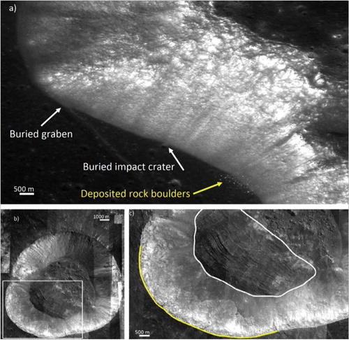
In this research, the recognition process of lunar landslides has been applied to detect slumps in simple impact craters, i.e. those cavities typically bowl-shaped and not affected by terraced rims (Melosh, 1989), secondary impacts or heavily degraded. Figure 1 shows some examples of slumps in lunar impact craters.

Figure 1. Some examples of lunar slumps: (a) a slump along the promontorium Laplace where the deposit has buried a small crater and part of graben (white arrows); the traces of a few fallen boulders due to a subsequent rock fall can be noted as well (yellow arrows); (b) a slumped wall on the Crater Tharp; (c) a close up of the slump of Crater Tharp, in yellow is highlighted the crown and in white the deposit. Images obtained via QuickMap™ tool.

Geological, morphological, physical factors and even human activity on the Earth (e.g. road cuts) may lead to the instability of the surface features, and may be considered as predisposing factors for landslides. While multiple combined factors may concur to the instability of a slope, usually only a single triggering factor is responsible for the landslide occurrence. The triggering factors for lunar landslides are distinctively different from the ones on the Earth. The large number of various size meteorite impacts are considered as the main direct triggering factor for mass movements on the Moon. These may also act as predisposing factors. Indeed, impacts may induce shock waves that directly disturb materials on slopes forming mass wasting landforms (Lindsay, 1976). This process may result in crushed subsurface bedrock and formation of fractured zones that sometimes extend for several times the crater radius beneath the crater floor (Melosh, 1989). In such a weakened region, a landslide may be triggered in a second stage by another impact in the nearby or by a moonquake.

After reviewing of recent missions to the Moon and the available data sets in Section “Recent missions to the moon and data applied in the work,”, it turns out that a consolidated methodology for the automatic or semi-automatic recognition of landslides in lunar impact craters has not been defined yet (see Section “Visual detection of landslides within simple impact craters”). Consequently, a new method based on the approximation of crater cross-sectional profiles with Chebyshev polynomials is described in Section “Landslide recognition based on the Chebyshev polynomials .” Thanks to the analysis of the asymmetry of such profiles, the presence of landslide features in lunar impact craters is recognized. Experimental results are reported in Section “Application 1 along with GLD100,” while Section “Conclusions and future developments” hosts discussions and some final considerations.

Recent missions to the moon and data applied in the work

For centuries, mankind has been interested in studying the Moon, but it was only in the middle of the 20th century that the first space missions and probes started approaching the Earth’s satellite. In the last decade, with the help of the major space agencies and their exploration missions, scientists started to have access to huge data sets holding the potential for unprecedented scientific discoveries (Zinzi et al., 2016) . At present, three ongoing lunar missions must be mentioned: the Lunar Reconnaissance Orbiter (LRO) by National Aeronautics and Space Administrations (NASA, United States), the SELenological and ENgineering Explorer (SELENE-KAGUYA) by the Japan Aerospace Exploration Agency (JAXA, Japan), and Chang’E missions by the Chinese Nationals Space Administration (CNSA, P.R. China). LRO (Chin et al., 2007; Robinson et al., 2010) and SELENE-KAGUYA (Araki et al., 2007) are orbiters with on-board measuring instruments. Chang’E is an ambitious program composed of several missions dedicated to the exploration of the Moon. The first missions in the series (Chang’E-1 and Chang’E-2) had the main aims of providing a digital elevation model (DEM) of the lunar surface and mapping the abundance and distribution of various chemical elements [Sun et al., 2005]. Chang’E-3 (Li, Liu, et al., 2015) is an unmanned exploration mission incorporating a robotic lander and a rover (Yutu), that has already travelled 114 m on the lunar surface.

LRO has six individual instruments on-board, with the purpose of producing accurate maps and obtain high-resolution images, to assess potential future landing sites and lunar resources, and to characterize the radiation environment (Chin et al., 2007). The instrumental payload on-board LRO also includes the Lunar Reconnaissance Orbiter Camera (LROC), consisting of two Narrow-Angle Cameras (NAC’s) and a Wide-Angle Camera (WAC). NAC’s ground sampling distance (GSD) may reach 0.5 m pixel size over a 5 km swath, while WAC provides images at average GSD of 100 m over a 60 km swath in seven spectral bands. As a result from the WAC stereo images a nearly global DEM with a resolution 100 m x 100 m was produced using photogrammetric image matching (GLD100), see (Scholten et al., 2012). This DEM covers 98.2% of the entire lunar surface, with an average elevation accuracy in the order of ±20 m, which may be even better than ±10 m in the maria. The GLD100 as well as WAC and NAC images were used for the study of landslide features on the lunar surface. Such data sets could be accessed through the QuickMap™ web interface (http://target.lroc.asu.edu/q3/) and the open source Java Mission-planning and Analysis for Remote Sensing (JMARS) software. This is a WEB-GIS platform developed by the Arizona State University (http://jmars.asu.edu/) that allows handling planetary remote-sensing data sets.

Visual detection of landslides within simple impact craters

While the automatic identification of lunar impact craters has been successfully achieved (Kang, Luo, Hu, & Gamba, 2015; Vijayan, Vani, & Sanjeevi, 2013; Li, Ling, et al., 2015), to date the detection and mapping of lunar landslides has been obtained only through visual inspection of images (e.g. Brunetti et al., 2015; Xiao et al., 2013). The recognition and mapping of landslides on the Moon surface adopted the same visual interpretation criteria used by geomorphologists to detect and map terrestrial landslides (Antonini et al., 2002; Rib & Liang, 1978; Speight, 1977; Van Zuidam, 1985). For the visual detection and mapping of landslides in impact craters, Brunetti et al. (2015) started with a recognition of the general landscape (e.g. local slopes, terrain steepness) in the areas of the selected crater using available images and DEM’s. Then, they extracted several topographic profiles from the DEM, thus allowing the morphology analysis of the crater and of the landslide, and more specifically, the detection of the landslide boundaries. Thereafter, they drew a circle that approximated the crater circumference, to detect the deformation of the crater rim induced by the landslide. The size of the circle was set according to the curvature of the non-collapsed crater rim. Finally, the landslide scarp and deposit were mapped (see examples from Brunetti et al. (2015) in Figure 2).

Figure 2. Examples of landslides mapped in two lunar craters. Figures (a) and (b) portray Gerasimovich D; (c) and (d) Cassini A craters. The blue circle approximates the crater rim; purple and green shaded areas are the landslide scarp and deposit, respectively. Credits: (Brunetti et al., 2015) and NASA/Goddard Space Flight Center/ASU.

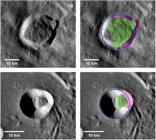
Brunetti et al. (2015) estimated a 20% uncertainty in the geometric measurement of the landslide area. This uncertainty is ascribed to the complex morphology of the lunar terrain, and to the resolution of images used to detect and map slope failures. In addition, the frequent presence of elongated shadows or overexposed areas prevents the correct identification of landslide boundaries.

Landslide recognition based on the Chebyshev polynomials

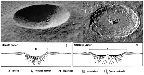
Since the presence of an enormous amount of impact craters on the Moon where slumps might have occurred, the definition of a methodology that automatically provides at least a preliminary recognition of such mass wasting processes is still called for. In the previous section, the visual analysis of optical images has proven to be efficient for slump recognition. In the experience of the authors, the visual analysis of optical images works well in the case of interpretation by an expert geologist, but it is highly error prone when some pattern recognition algorithms are applied. Crater geometry could potentially provide more robust information when implemented in an automatic recognition process rather than using images. Any significant deviation of the crater geometry from the original shape of the simple bowl-shaped crater may be interpreted as the presence of a landslide. As it can be seen in Figure 3, the morphology of impact craters might also be quite complex with terraced margins and central peaks (Melosh H.J., 1989) and in such a case the recognition of slumps is more difficult. Also, the impact angle of the meteorite, the sloped terrain, and the degradation processes in the crater may have led to situations where the presence of a slump may be masked, or where morphologies similar to the ones due to slumps may be found. Such cases would easily result in omission and errors during classification. For this reason, the algorithm presented in the following is supposed to work for simple craters having approximately circular shape. These might have resulted from the impact of meteorites whose trajectory is not lower than 10° with respect to the horizontal plane, as stated in Melosh (2011).

Figure 3. Example of different types of lunar craters, from the simplest one consisting in a single bowl-shape (at the upper left side crater Linné) up to complex craters (at the upper right side crater Tycho). General structure of (c) simple crater and (d) complex crater. Credits: NASA/Goddard/Arizona State University.

Polynomial approximation has been used in Mahanti, Robinson, Humm, and Stopar (2014) to find a characterization of crater cross-sectional profiles. This method can be classified as data-driven, since it does not need any a priori model to be assumed. Since the approximation of more complex shapes of the profiles can be done by simply increasing the order of the approximating polynomial, this solution is potentially efficient also in the case of craters affected by soil degradation processes. The approximation level depends on the degree of the adopted polynomials: the terms that are omitted give rise to the so called truncation error, whose magnitude is related to the specific implemented polynomials. In Mahanti et al. (2014) the Chebyshev polynomials (Mason & Handscomb, 2010) have been used for approximating craters’ cross-sectional profiles. Since the presence of a slump in a crater may alter the symmetry of the profiles intersecting the slump’s body, the analysis of symmetry might be used for recognition, as in Mahanti, Robinson, and Thompson (2015). The development of the idea, that was briefly introduced in Mahanti et al. (2015), is presented here, after providing a short review on Chebyshev polynomials’ mathematical background and their basic properties.

Background on Chebyshev polynomials

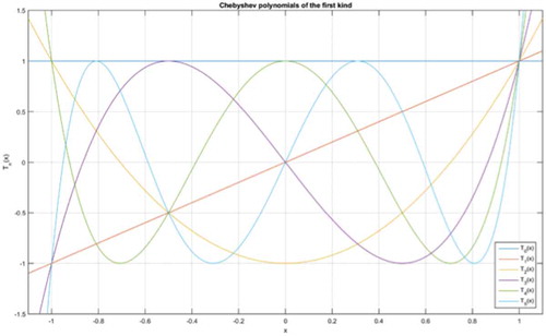
The Chebyshev polynomials are a series of orthogonal polynomials, each of them featuring a unique and uncorrelated shape with respect to any other members of the series. Following (Mahanti et al., 2014), the so called Type I Chebyshev polynomials have been adopted for approximating crater cross-sectional profiles. This is motivated by the great simplicity of the coefficients related to this representation. The formulation of polynomials’ basis functions is based on a recursive series defined in the domain between −1 and +1:

(1)

where T_n(x) is the polynomial basis function of order n. The basis functions of order n = 0 and n = 1 are T₀(x) = 1 and T₁(x) = x, respectively. In Figure 4, the graphical plot of the six basis functions of Chebyshev polynomials are shown.

Figure 4. Graphical plots of the first six basis functions of Chebyshev polynomials (in different colours).

In order to approximate a real function f(x), a linear combination pM(x) of the first M + 1 basis functions of Chebyshev polynomials is adopted:

(2)

where M is the degree of the Chebyshev polynomial and C_n are the coefficients that modulate the amplitude of each basis component. Coefficients C_n are estimated on a least-squares basis to fit with real profile data, as discussed in subsection ‘Landslide recognition using Chebyshev polynomials’. The residual approximation error o(x_M) is equal to the sum of missing terms after degree M that are not considered in the approximation (i.e. truncation error).

As it results from Equations (1) and (2), in the Chebyshev polynomial series even (symmetric w.r.t. vertical axis) and odd (anti-symmetric) basis functions alternatively appear. Consequently, the size of odd coefficients may express the degree of asymmetry of the approximated function f(x).

Several properties make the Chebyshev polynomials particularly efficient for approximating crater cross-sectional profiles. These could be summarized in five main points:

(i) The basis functions are mutually orthogonal and the estimated coefficients are uncorrelated. This property results in the consequence that, even though the total number of adopted coefficients may be different, the estimated values of the lower order coefficients it is always the same. This property is important because it makes the estimated coefficients independent from the specific estimation process, hence they can be compared in a meaningful way among several cross-sectional profiles. Indeed, lower numbered coefficients C_n have a larger impact in the approximation of the crater profile geometry.

(ii) Chebyshev polynomials may well fit to the interpolated function f(x), i.e. the crater cross-sectional profile (Gautschi, 2004; Mason & Handscomb, 2010), if a proper number of basis functions/coefficients is selected; consequently, residuals may also be very small, depending on the number of adopted coefficients. Taking advantage of this property, Mahanti et al. (2014) demonstrated that lunar crater cross-sectional profiles could be approximated by using the first 17 coefficients (M = 16) of Chebyshev polynomials.

(iii) Extreme values of Chebyshev polynomials always occur at some specific positions on the reference axis (x = −1, 0, +1). This property makes easier to link the estimated polynomials’ coefficients with the geometry of the crater.

(iv) Correlation among the lower order coefficients as well as some combinations of coefficients with some important morphological properties of the crater and its surrounding terrain exist (average crater profile elevation, local topographic gradient, crater depth, etc.), see (Mahanti et al., 2014). This does not mean that morphological features can be directly obtained from Chebyshev coefficients, but that a set of numerical shape indicators can be related to some morphological properties, through a repeatable almost automatic process.

(v) Detection of asymmetry in the crater cross-sectional profile is possible on the basis of the analysis of odd polynomials’ coefficients.

Landslide recognition using Chebyshev polynomials

In this subsection, the description of the algorithm conceived for slump landslide recognition is presented, while next section on “Application 1 along with GLD100” will demonstrate its application. The general workflow that is followed is shown in Figure 5, while in Figure 6 different steps of the analysis of a lunar crater are reported.

Figure 5. Workflow of the algorithm adopted to detect the presence of a slump in a cross-sectional profile of a lunar crater.

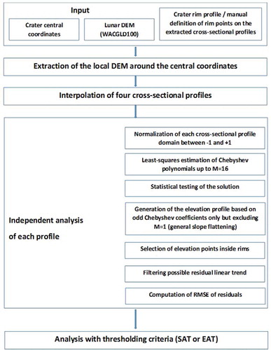
Figure 6. Application of the algorithm described in the workflow in Figure 5 to analyse a cross-sectional profile of crater Moseley C, West–East direction.

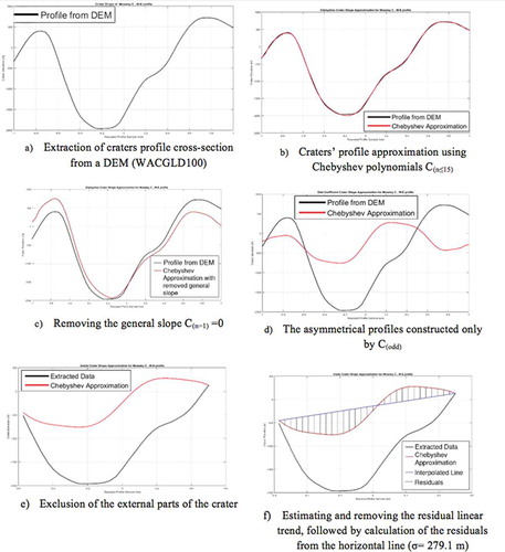
The approximation of each profile is accomplished by considering a cross-section extending outside the crater rims to include a small portion of outer terrain. The distance between both extremes of the profile is then normalized in the interval −1 and +1, being this the domain of Chebyshev polynomials, see Equation (1). In the case under consideration, the function to approximate is the discrete crater profile f(x_i), being x the sample direction. Points along the cross-sectional profile must be regularly spaced at the same sampling resolution. Each profile can be extracted from a DEM, in this case the GLD100.

The input is given by the central geographic coordinates (latitude φ_cc, longitude λ_cc) of the crater with respect to the lunar ellipsoid (Edwards et al., 1996) and the crater cross-sectional profile. Both can be obtained from existing databases (e.g. Losiak et al., 2009), from previous studies (e.g. Brunetti et al., 2015), or simply by manual selection on a digital georeferenced map.

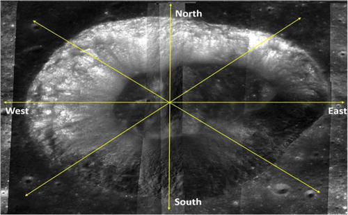
Using this input information, the digital surface model of the whole crater is extracted from a lunar DEM, including an outer region since the profile to extract may comprehend also a portion of external terrain. A window equal to approximately 50% of the profile outside both rims has been adopted here to extract the crater DEM from the global DEM (GLD100). This intermediate step is motivated by the fact the global DEM may also be online, thus first a portion of DEM comprehending the crater is downloaded, then four cross-sectional profiles are manually extracted at 45° relative orientation steps starting from North–South direction, see Figure 7. It has been proven that four profiles are enough for detecting a large mass wasting feature, i. e. slump, while for the purpose of more detailed analyses (e.g. determining the landslide boundaries or the volume of the deposit) higher number of cross-sectional profiles could be considered as useful. Since the slope of lunar DEM is in general quite smooth and flat, a bilinear interpolation of the four closest points is used to derive the elevation h_i of point ith in each cross-sectional profile. Along each profile, points are interpolated at regular spacing δ. The total length of the profile depends on the rim-to-rim distance and maybe uneven for different cross-sections related to the same crater. Indeed, the shape of a crater may be elongated along one direction because of the presence of a slumped wall. An extension of the profile length approximately equal to 30% of the rim-to-rim distance is adopted here. In order to tailor the extraction of cross-sectional profiles, a precise model for the crater rim shape should be applied at this stage. As an alternative, the position of the crater’s rims on each profile may be manually picked up.

Figure 7. Example of extraction of four cross-sectional profiles to be analysed in the case of Moseley C crater (background image mosaicked from NAC LROC images).

The Chebyshev polynomial coefficients are estimated here using a standard Least-squares approach. Following the results discussed in Mahanti et al. (2014), coefficients up to order M = 16 are enough for the characterization of the crater morphology. Details about this stage can be found in Yordanov et al. (2016), as well as reports about statistical testing to assess the quality of the interpolation.

Since the coefficient with M = 0 gives the average normalized elevation of the cross-sectional profile and the coefficient with M = 1 gives the general slope, both can be used to shift the elevation around zero mean and to flatten the profile shape. This task helps the application of the criteria for the analysis of the asymmetric component that will be introduced in the following. Indeed, the sum of polynomial members corresponding to odd coefficients represents the asymmetric component of the profile, which is supposed to be due to the presence of a slump. Indeed, in the case no slump has developed inside the crater, the Chebyshev approximation should mainly consist of non-zero even coefficients, while the odd coefficients should be close to zero. On the contrary, in the case a slump is present, the odd coefficients should be significantly different from zero. Testing the size or the statistical significance of the odd coefficients should theoretically be a direct way to detect symmetry. After a few experiments already reported in Yordanov et al. (2016), the analysis of odd coefficients did not provide satisfying results. This was due to the presence of noise and other local effects in the inner crater topography, which may have caused the odd coefficients to be significantly different from zero even in the case a slump was not present. As an alternative, the analysis of the odd Chebyshev coefficients’ absolute size demonstrated to be a more effective way to detect the presence of a significant asymmetric component, then the possible existence of a slump. To carry out such an analysis for a given cross-sectional profile, the contribution of the odd coefficients to the interpolated elevation is computed for any points at position x_i located inside the crater (x_min < x_i < x_max, being x_min and x_max the positions of the rim edges in the profile):

(3)

Here the basis function corresponding to M = 1 is omitted since this describes the general slope to be flattened. On the other hand, successive basis functions may describe asymmetries inside the crater and thus are considered in the analysis.

Secondly, the Root Mean Square Error (RMSE) of all elevations h_i is computed for the cross-sectional profile sec:

(4)

where is the number of points located inside the rim-to-rim sector.

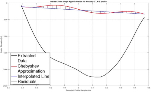
Since the RMSE_sec should be small in the case of the absence of a slump (see Figure 8) and large in the presence of a slump (see the last subfigure in Figure 6), the RMSE_sec is tested against a threshold established to operate the landslide recognition. Thresholds can be defined on a statistical basis or on an empirical basis, coming from the observation of cross-sectional profiles that are really affected by slumps. The selection of the threshold type is directly connected to the adopted data set. For this reason, this discussion is done in the experimental Section ‘Application 1 along with GLD100’.

Figure 8. Residuals of the cross-sectional profile estimated on the basis of odd Chebyshev polynomials coefficients with respect to the original profile in the case of crater Moseley C, North–South direction, which does not include a slump.

Since the bottom of a crater may contain a low-frequency component due to the accumulation of sediment rather than to large sudden slope failures, the presence of a regular linear trend may be detected and removed before the analysis of odd elevation h_i.

Application along with GLD100

During this study a total amount of 51 lunar impact craters (Figure 9) have been analysed to detect the presence of slumps. Among these, 31 had been already classified as affected by landslides (Brunetti et al., 2015), while 20 additional craters without slumps have been investigated for the purpose of having a more consistent data set including either profiles “with landslides” and “without landslides.” These last craters have been chosen on a visual-interpretation basis, and with diameter in the range between 7 and 16 km. The diameters of the 51 craters have the following dimensions: 10 craters have diameter between 7 and 10 km, 11 between 10 and 15 km, 12 between 15 and 20 km, 10 between 20 and 25 km, 5 between 25–30 km and 3 craters between 30 and 37 km. Even though, in the literature (Melosh 2011) a simple crater on the Moon is in the range up to 20 km of diameter, in this work larger craters were considered as well due to the fact they did not show those features typical of a complex crater such as central peaks or terraced walls. Nevertheless, we acknowledge that landslides mapped in larger craters could be incomplete terracing due to complex crater formation during the modification stage (Brunetti et al., 2015). The total number of extracted cross-sectional profiles including all four directions has been 204. Each cross-section has been made up of points at linear sampling distance of 200 m, given an original spatial resolution of the adopted DEM 100 m × 100 m. The reduction of resolution was decided to smoothen each section in order to mitigate local noise, and to consider that a cross-section direction may also be non-parallel with respect to the DEM grid axes.

Figure 9. Location of the lunar impact craters selected to be part of the analysis for detecting inner slumps.

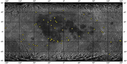
The selection of the impact craters to analyse has been done to have a data set sharing common features:

● Simple bowl-shape crater type;

● Size of the maximum crater diameter ranging from 7 km up to 20 km, with some exception up to a diameter of 37 km but with simple bowled shape;

● Maximum slope inside the crater below 35°; and

● Almost circular shape of the crater.

Through visual recognition each cross-sectional profile has been classified as “with landslide” or “without landslide.” In total, 65 cross-sections have been classified as “with landslide” and 139 “without,” respectively. Using such a data set made up of both types of cross-sectional profiles, the efficiency of the algorithm to detect slumps against omission and commission errors can be evaluated.

As previously mentioned, two threshold criteria have been proposed to scrutinize the presence of slumps. Indeed, one of the aims of the test within the case study presented above has been to find which threshold would perform better. Both thresholds are designed to analyse the obtained residuals after interpolation and filtering process. In particular, the RMSE_sec of residuals, which is expected to be close to zero in the case there is not a landslide in the crater, is analysed. The problem is to decide which is the threshold on the RMSE_sec in each individual cross-section. A desired result was to define on one side an unique threshold value, whether adaptive or fixed, in order to be able to analyse different craters under the same conditions. On the other, to establish a numerical procedure for detecting slumps, omitting the human factor throughout the process of analysis. Of course, the presence of noise and the local topographic anomalies make this analysis more complex.

Statistical adaptive thresholding method

The statistical adaptive thresholding (SAT) criterion defines an adaptive threshold depending on each separate impact crater. Thresholding is based on the statistical analysis of all four cross-sectional profiles extracted from the same crater. The basic hypothesis is that the presence of a slump should not affect all cross-sections. Consequently, by comparing the RMSE_all computed on all profiles with the ones computed on a single profiles (RMSE_sec), it should be possible to point out the presence of a slump. A scaling factor k has been introduced, where k ranges from 0.8 and 1.35. The condition for recognizing a landslide in an individual cross-sectional profile is that:

(5)

Empirical absolute thresholding method

The empirical absolute thresholding (EAT) criterion defines a fix threshold disregarding, which is the impact crater under analysis. In addition, all four cross-sectional profiles are checked against the same threshold. The adopted values applied to the case study range from 100 to 170 m at 10 m steps. The proposed values range was obtained after testing a much wider spectrum (from 50 to 300 m) and due to not satisfactory results was narrowed down to one described previously.

While in the future development of this research a way to link the empirical threshold to some observable physical properties should be investigated, so far these thresholds have been simply guessed by looking at the size of residuals in the odd coefficient profiles.

Results and discussion

The process for interpolation of crater cross-sectional profiles based on Chebyshev polynomials and the successive computation of RMSE of residuals has been applied to all 51 craters belonging to the case study. The analysis of RMSE has been repeated with both types of thresholding methods and different threshold values. In this manner, all possible combinations were obtained and the achieved results were not influenced by any outer factors. Results are summarized in Table 1.

Table 1. Overview of the results obtained in the classification of cross-sectional profiles as “with landslide” and “without landslide,” according to diverse thresholding methods and values.

		Landslides				No landslides
		True		False		True		False
Threshold method		Num	(%)	Num	(%)	Num	(%)	Num	(%)
SAT-adaptive	0.8 RMS	54	83.1	11	16.9	67	48.2	72	51.8
	1 RMS	52	80.0	13	20.0	83	59.7	56	40.3
	1.1 RMS	50	76.9	15	23.1	90	64.8	49	35.3
	1.15 RMS	47	72.3	18	27.7	97	69.8	42	30.2
	1.2 RMS	46	70.8	19	29.2	105	75.5	34	24.5
	1.25 RMS	43	66.2	22	33.9	106	76.3	33	23.7
	1.3 RMS	40	61.5	25	38.5	111	79.9	28	20.1
	1.35 RMS	38	58.5	27	41.5	116	83.5	23	16.6
EAT-absolute value	100	57	87.7	8	12.3	110	79.1	29	20.9
	110	55	84.6	10	15.4	116	83.5	23	16.6
	120	54	83.1	11	16.9	120	86.3	19	13.7
	130	52	80.0	13	20.0	122	87.8	17	12.2
	140	48	73.9	17	26.2	122	87.8	17	12.2
	150	46	70.8	19	29.2	127	91.4	12	8.6
	170	41	63.1	24	36.9	129	92.8	10	7.2

Disregarding the type of criterion applied, the selection of a higher threshold value has two opposite effects on the true detection of cross-sectional profiles “with landslide” and “without landslide”. These effects can be clearly seen in Figures 10 and 11. In the former case, the higher the threshold value, the lower the fraction of true classifications. In the latter case, the higher the threshold value, the higher the number of correct classifications. This result is quite logical, since the rising up of the threshold may lead to exclude from the classification as “with landslide” those cross-sectional profiles affected by smaller size slumps. The opposite effect is obtained when considering the classification of cross-sectional profiles “without landslide.” As this is what has happened about the omission errors according to the threshold values, complementary results can be observed in Figures 10 and 11 about commission errors. For instance, as far as the threshold value grows, the fraction of cross-sectional profiles “with landslide” that are not correctly classified increases. This finding means that appropriate thresholds should be applied when the objective is to seek for cross-sections affected by landslides or for profiles which are not affected.

Figure 10. Plots of results in terms of true/false successful classification (%) for both cases “with landslide” and “without landslide” when the empirical absolute thresholding (EAT) is used.

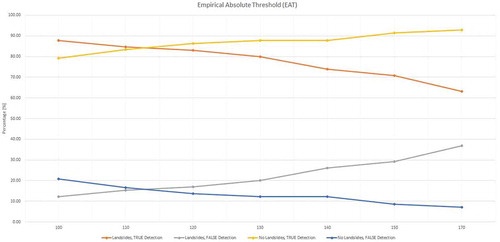
Figure 11. Plots of results in terms of true/false successful classification (%) for both cases “with landslide” and “without landslide” when the statistical adaptive thresholding (SAT) is used.

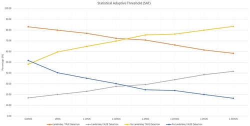
The empirical absolute threshold criterion has offered the best performance in the classification of cross-sectional profiles “without landslide.” Here a result of 92.8% (129 over 139 profiles) has been reached when using an EAT of 170 m, while SAT has provided the best result of 83.5% (116 over 139 profiles) when using a threshold value of k = 1.35·RMSE_all. When seeking for cross-sections “with landslide”, the EAT has rated 87.7% (57 over 65 profiles) of true classifications when using a threshold equal to 100 m, while SAT has provided 83.1% (54 over 65 profiles) of correct classifications in correspondence of a threshold k = 0.8. Omission errors are of course complementary to 100% of correct classifications. In addition, by looking at plots in Figures 10 and 11, a trade-off threshold value optimizing the number of correct classifications in the case of cross-sections “with” and “without landslide” may be set up at the intersection of lines describing the behavior of true classifications (i.e., red and yellow lines, respectively). For EAT, a threshold value of 113 m would give approximately 84% of correct classifications for both cases. For SAT, a threshold value k = 1.16 would give approximately 72% of correct classifications.

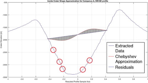
It should be noted that these results are preliminary and further analyses and expansion of the proposed method are necessary, in order to improve them. This is also to the fact that the variety of cases is huge and some features are wrongly detected, i.e. profiles “with” landslides are recognized as ones “without” and the opposite. But investigating these cases could improve future algorithms. In Figure 12 is represented the W-E profile of the crater Drebbel, with its RMSE_sec = 79.07 m, it was recognized as a profile “without” landslides (applied threshold EAT = 100 m). But one can clearly notice the fact that the profile is not clearly symmetric and a feature is interfering the expected bowl-shape. Addition visual analysis at the GLD100 confirmed the feature is a deposit of a collapsed western wall. But the deposit itself was not big enough to be detected by the method. On the other hand, Figure 13 represents the NW-SE profile of crater Schrodinger B, where the RMSE_sec = 133.08 m with again EAT = 100 m is recognized as profile “with” landslide. The feature appearing at the bottom of the crater could not be related to a landslide deposit. The high RMSE value could be related to the short-length dunes (red circles) previously detected as well in other craters (e.g. Yordanov et al. (2016)). An increasing of the number of craters’ profiles extracted from the DEM could improve the results and eliminate errors similar to the above discussed. As well, it can contribute for more precise determination whether the deposit is from one or more events, to delineate the boundaries of it and even to compute the displaced mass.

Figure 12. W-E profile of the crater Drebbel, with RMSEsec = 79.07 m and recognized by EAT = 100 m as profile “without” landslides.

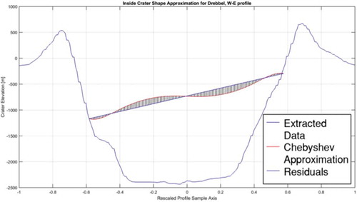
Figure 13. NW-SE profile of the crater Campanus A, with RMSEsec = 103.06m and recognized by EAT = 100 m as profile “with” landslides. The red circles are highlighting the short-length dunes.

Although both criteria have not output largely different results, in general the use of fixed thresholding (EAT) has demonstrated a slightly better performance. It should be also noticed that the selected impact craters share some homogenous properties (as described at the beginning of this section) and are evenly widespread on the entire surface of the Moon (see Figure 9). This leads to the conclusion that the choice of an EAT having a general validity among groups of similar craters is not a difficult task. On the other hand, the selection of a threshold value has been confirmed by using a set of pre-classified cross-sectional profiles for validation. In the development of this research it would be relevant, on one side to link the threshold values to some physical properties of cross-sectional profiles. On the other side, it would be important to extend the analysis to a wider sample of craters, in order to use a subset of pre-classified profiles to define proper thresholds to be extensively applied to non-pre-classified profiles as well. Anyway, the thresholds obtained from this study have been sufficiently proved to have a general validity, so that they will be suitable to be used in future research applications.

Conclusions and future developments

A methodology for the automatic recognition of landslides inside the impact craters on the Moon has been presented and discussed. In particular, the proposed technique works on the basis of Chebyshev polynomial approximations and it is designed for detection of slumps occurred after the meteorite impact that originated the crater. Such phenomenon generally leaves a significant modification of the crater topography, which in the most cases gives an asymmetric shape to the crater itself. The analysis of the odd components of the Chebyshev polynomials is exploited to detect the possible presence of a slump. This procedure is applied to approximate topographic cross sections extracted from four cross-sectional profiles from a global lunar DEM (GLD100).

The best performance in term of successful slump recognition has been obtained when using an empirical absolute threshold (EAT) for discriminating those cross-sectional profiles affected by landslides from others. During the analysis of a case study, 92.8% of cross-sections containing a slump have been correctly classified in almost automatic way, barring the preparation of input data and the definition of crater rims, which is still currently a manual task. Even though non-exhaustive results have been obtained, the analysis could be used as preliminary processing step to be refined afterwards. This option may be relevant to the production of a complete map of slumps in impact craters on the entire Moon or other planetary bodies.

On the other hand, in order to mitigate the number of wrong classification errors, two different actions should be undertaken. On one side, a better definition of the threshold for discriminating those cross-sectional profiles comprehending a slump should be operated. In particular, linking the EAT to some physical properties of the crater morphology and to data quality is expected to give a positive contribution. On the other side, other analyses based on complementary data sources would help make the recognition process more robust. For instance, the use of multispectral data from Chinese Chang’E-1 mission has offered some initial interesting results for the detection of spectral anomalies along the slopes of craters, which can be linked to lithological and morphological different features (Scaioni et al., 2016).

Also some improvements to rise up the level of automation of the whole procedure are needed. One of them consists in the integration of some techniques for extracting craters’ rims and other geomorphological features that help the landslide recognition algorithm.

Acknowledgements

The main acknowledgements go to the Italian Space Agency and the Center of Space Exploration of China Ministry of Education which have promoted, funded and supported this project. Acknowledgements also go to all administrations of Italian and Chinese universities and research centres involved in ‘Moon Mapping Project.’ The authors would like to sincerely thank the Embassy of Italy in Beijing and especially the Science & Technology Counsellor (Professor Plinio Innocenzi). The authors would also thank all those colleagues who have been supporting in some way the research or the organizational activities. Finally, many thanks go to students who effectively contributed to this project.

Disclosure statement

No potential conflict of interest was reported by the authors.

Additional information

Funding

This work was supported by the Italy-China Cooperation project “Moon Mapping” (Italian Space Agency – ASI), 2014-2017.

References

- Antonini, G., Ardizzone, F., Cardinali, M., Galli, M., Guzzetti, F., & Reichenbach, P. (2002). Surface deposits and landslide inventory map of the area affected by the 1997 Umbria–Marche earthquakes. Bollettino Società Geologica Italiana, 121(2), 843–853.
- Araki, H., Tazawa, S., Noda, H., Tsubokawa, T., Kawano, N., & Sasaki, S. (2008). Observation of the lunar topography by the laser altimeter LALT on board Japanese lunar explorer SELENE. Advances in Space Research, 42, 317. doi:10.1016/j.asr.2007.05.042
- Bart, G.D. (2007). Comparison of small lunar landslides and Martian gullies. Icarus, 187, 417–421. doi:10.1016/j.icarus.2006.11.004
- Brunetti, M.T., Guzzetti, F., Cardinali, M., Fiorucci, F., Santangelo, M., Mancinelli, P., & Borselli, L. (2014). Analysis of a new geomorphological inventory of landslides in Valles Marineris, Mars. Earth and Planetary Science Letters, 405, 156–168. doi:10.1016/j.epsl.2014.08.025
- Brunetti, M.T., Xiao, Z., Komatsu, G., Peruccacci, S., & Guzzetti, F. (2015). Large rockslides in impact craters on the Moon and Mercury. Icarus, 260, 289–300. doi:10.1016/j.icarus.2015.07.014
- Buczkowski, D.L., Schmidt, B.E., Williams, D.A., Mest, S.C., Scully, J.E.C., Ermakov, A.I., … Russell, C.T. (2016). The geomorphology of Ceres. Science, 353(6303), aaf4332. doi:10.1126/science.aaf4332
- Chin, G., Brylow, S., Foote, M., Garvin, J., Kasper, J., Keller, J., … Zuber, M. (2007). Lunar reconnaissance orbiter overview: The intrument suite and mission. Space Science Review, 129, 391–419. doi:10.1007/s11214-007-9153-y
- Cruden, D.M., & Varnes, D.J. (1996). Landslide types and processes. Transportation Research Board, National Academy of Sciences, 247, 36–75.
- De Blasio, F.V. (2011). Landslides in Valles Marineris (Mars): A possible role of basal lubrication by sub-surface ice. Planetary Space Science, 59, 1384–1392. doi:10.1016/j.pss.2011.04.015
- Edwards, K.E., Colvin, T.R., Becker, T.L., Cook, D., Davies, M.E., Duxbury, T.C., … Sorensen, T. (1996). Global digital mapping of the Moon. 27th Lunar and Planetary Science Conference (1996), Abstract #1168.
- Gautschi, W. (2004). Orthogonal polynomials: Computation and approximation. USA: Oxford University Press.
- Jay, M.H. (2011). Planetary surface processes (Vol. 13). Cambridge, Cambridge University Press.
- Kang, Z., Luo, Z., Hu, T., & Gamba, P. (2015, October). Automatic extraction and identification of lunar impact craters based on optical data and DEMs acquired by the Chang’E satellites. IEEE Journal of Selected Topics in Applied Earth Observations and Remote Sensing, 8(10), doi:10.1109/JSTARS.2015.2481407
- Krohn, K., Jaumann, R., Otto, K., Hoogenboom, T., Wagner, R., Buczkowski, D.L., … Raymond, C.A. (2014). Mass movement on Vesta at steep scarps and crater rims. Icarus, 244(2014), 120–132. doi:10.1016/j.icarus.2014.03.013
- Li, B., Ling, Z.C., Zhang, J., & Wu, Z.C. (2015). Automatic detection and boundary extraction of lunar craters based on LOLA DEM data. Earth Moon and Planets, 115, 59–69. doi:10.1007/s11038-015-9467-9
- Li, C., Liu, J., Ren, X., Zuo, W., Tan, X., Wen, W., … Ouyang, Z. (2015). The Chang’e 3 mission overview. Space Science Reviews, 190, 85–101. doi:10.1007/s11214-014-0134-7
- Lindsay, J. (1976). Energy at the lunar surfaces. In Z. Kopal & A.G.W. Cameron (Eds.), Lunar stratigraphy and sedimentology. In: Developments in Solar System and Space Science, vol.3. Amsterdam Marco: Elsevier, pp.45–55.
- Losiak, A., Wilhelms, D.E., Byrne, C.J., Thaisen, K., Weider, S.Z., Kohout, T., … Kring, D.A. (2009). A new lunar impact crater database. Lunar Planet. Sci., 40, no. 1532.
- Mahanti, P., Robinson, M., Humm, D., & Stopar, J. (2014). A standardized approach for quantitative characterization of impact crater topography. Icarus, 241, 114–129. doi:10.1016/j.icarus.2014.06.023
- Mahanti, P., Robinson, M., & Thompson, T. (2015). Characterization of lunar crater wall slumping from Chebyshev approximation of lunar crater shapes. In Annual meeting of the Lunar Exploration Analysis Group (LEAG), Abstract 2081. LPI Contribution No. 1863, Lunar and Planetary Institute, Houston.
- Mason, J., & Handscomb, D. (2010). Chebyshev polynomials. FL: CRC Press Company.
- Massironi, M., Marchi, S., Pajola, M., Snodgrass, C., Thomas, N., Tubiana, C., … Koschny, D. (2012). Geological map and stratigraphy of asteroid 21 Lutetia. Planetary and Space Science, 66, 125–136. doi:10.1016/j.pss.2011.12.024
- Mazzanti, P., De Blasio, F.V., Di Bastiano, C., & Bozzano, F. (2016). Inferring the high velocity of landslides in Valles Marineris on Mars from morphological analysis. Earth, Planets and Space, 68(1). doi:10.1186/s40623-015-0369-x
- Melosh, H. (1989). Impact cratering: A geologic process. New York: Oxford University Press.
- Oberst, S.F., Matz, J., Roatsch, K.-D., Wählisch, T., Speyerer, E.J., & Robinson, M.S. (2012). GLD100: The near-global lunar 100m raster DEM from LROC WAC stereo image camera. Journal of Geophysical Research, (117), E00H17. doi:10.1029/2011JE003926
- Pike, R.J. (1971). Some preliminary interpretations of lunar mass-wasting processes from Apollo 10 photography. Analysis of Apollo 10 photography and visual observations (Vols. NASA-SP-232, pp. 14–20). Washington, D. C: NASA Spec. Publ.
- Quantin, C., Allemand, P., & Delacourt, C. (2004). Morphology and geometry of valles marineris landslides. Planetary Space Science, 52(11), 1011–1022. doi:10.1016/j.pss.2004.07.016
- Rib, H.T., & Liang, T. (1978). Recognition and identification. In R.L. Schuster & R.J. Krizek (Eds.), Landslide analysis and control: Transportation research board special report, 176 (pp. 34–80). Washington: National Academy of Sciences.
- Robinson, M.S., Brylow, S.M., Tschimmel, M., Humm, D., Lawrence, S.J., Thomas, P.C., … Hiesinger, H. (2010). Lunar Reconnaissance Orbiter Camera (LROC) instrument overview. Space Science Reviews, 150(1–4), 81–124. doi:10.1007/s11214-010-9634-2
- Scaioni, M., Giommi, P., Brunetti, M.T., Carli, C., Cerroni, P., Cremonese, G., … Wu, Y. (2016). The ‘Moon mapping’ project to promote cooperation between students of Italy and China. Archives of the Photogrammetry, Remote Sensing and Spatial Information Sciences, XLI-B6, 71–78. doi:10.5194/isprs-archives-XLI-B6-71-2016
- Sentil Kumar, P., Keerthi, P., Sentil Kumar, A., & Mustard, J. (2013). Gullies and landslides on the Moon: Evidence for dry-granular flows. Journal of Geophysical Research, Planets, 118, 206–223. doi:10.1002/jgre.20043
- Speight, J.G. (1977). Landform pattern description from aerial photographs. Photogrammetry, 32, 161–182. doi:10.1016/0031-8663(77)90012-6
- Van Zuidam, R.A. (1985). Aerial photo-interpretation in terrain analysis and geomorphologic mapping. International Institute for Aerospace Survey and Earth Sciences (ITC) (pp. 442). The Hague: Smits Publishers.
- Vijayan, S., Vani, K., & Sanjeevi, S. (2013). Crater detection, classification and contextual information extraction in lunar images using a novel algorithm. Icarus, 226, 798–815. doi:10.1016/j.icarus.2013.06.028
- Waltham, D., Pickering, K.T., & Bray, V.J. (2008). Particulate gravity currents on Venus. Journal of Geophysical Research, Planets, 113, E2. doi:10.1029/2007JE002913
- Williams, D.A., O’Brien, D.P., Schenk, P.M., Denevi, B.W., Carsenty, U., Marchi, S., … Davison, T.M. (2013). Lobate and flow-like features on asteroid Vesta. Planetary Space Science. doi:10.1016/j.pss.2013.06.017
- Xiao, Z., & Komatsu, G. (2013). Impact craters with ejecta flows and central pits on Mercury. Planetary and Space Science, 82-83, 62–78. doi:10.1016/j.pss.2013.03.015
- Xiao, Z., Zeng, Z., Ding, N., & Molaro, J. (2013). Mass wasting features on the Moon–How active is the lunar surface? Earth and Planetary Science Letters, 376, 1–11. doi:10.1016/j.epsl.2013.06.015
- Yordanov, V., Scaioni, M., Brunetti, M.T., Melis, M.T., Zinzi, A., & Giommi, P. (2016). Mapping landslides in lunar impact craters using Chebyshev polynomials and Dem’s. International Archives of the Photogrammetry, Remote Sensing and Spatial Information Sciences, XLI-B6, 17–24. doi:10.5194/isprs-archives-XLI-B6-17-2016
- Zinzi, A., Capria, M.T., Palomba, E., Giommi, P., & Antonelli, L.A. (2016). MATISSE: A novel tool to access, visualize and analyse data from planetary exploration missions. Astronomy and Computing, 15, 16–28. doi:10.1016/j.ascom.2016.02.006