Monitoring heterogeneous urban and rural area using Normalised Difference Infrared Index – a case study from SE Poland

ABSTRACT

The results of a study of NDII applicability for monitoring of a heterogeneous rural and urban area during a growing season (April–November) were shown. We evaluated the spatial and quantitative distributions, and temporal trends of NDII derived from Landsat 8 imagery, NDII = (NIR–SWIR)/(NIR+SWIR) or NDII = (Band5–Band6)/(Band5+Band6), over a typical medium-sized European city with its surroundings. The temporal changes of NDII were also correlated with sunshine duration, temperature, and precipitation. Vegetation was the component of land cover that was changing to the highest degree during the growing season. The most dynamic temporal alterations of NDII were recorded within the arable land. In forest areas and grassland NDII was relatively stable through the summer. The NDII values were stable also in the built-up area in view of practically constant state of human-made covers in the studied period. NDII can support the monitoring of land cover/land use in the urban and rural areas, provided that the images of fully developed plant cover are used. It was stated that NDII correlated with weather conditions. The relationships between NDII and precipitation, temperature, and sunshine duration could facilitate risk assessment and planning of agronomic practices with regard to the weather.

KEYWORDS:

• NDII
• arable land
• grassland
• forest
• weather conditions
• Landsat satellite imagery

Introduction

The landscape of Europe is characterized by numerous medium-sized cities with up to 500,000 citizens. A typical feature of land cover/land use (LCLU) in the surroundings of European urban areas is large heterogeneity on the regional scale. The suburban areas form a mosaic of ecosystems: arable land, forests and other wooded areas, grassland, surface water that fulfil various functions for the city and serve the needs of its residents. A vital element of the discussed areas is vegetation which plays an important role in environment by promoting quality of life through: alleviating air pollution, soil erosion, excessive insolation and noise, protecting biodiversity, and maintaining ecological balance (Nabielek, Hamers, & Evers, 2016). Therefore, monitoring the vegetation condition is an essential element of rational spatial planning and land management.

The land and vegetation over the wide area can be observed by satellite remote sensing. For the analysis of variation in canopy status in respect to its condition and water content, images showing the reflectance in red (R), near (NIR), and shortwave (SWIR) infrared light are commonly used. The red band is sensitive to chlorophyll concentration, the NIR band is sensitive to plant tissue structure or biomass, and the SWIR is sensitive to water content in vegetation and soil (Hardisky, Klemas, & Smart, 1983). Therefore, a combination of the reflectance in the R, NIR, and SWIR band yields a number of indices widely used in the synoptic monitoring of vegetation intra- and inter-annual phenology in a variety of ecosystems: cropland, forests, grassland, urban greenery, etc. This subject is widely discussed and researched by many scientists. Dusseux, Vertès, Corpetti, Corgne, and Hubert-Moy (2014) studied grassland management practices in an intensive agricultural watershed located in Brittany, France. The authors analysed the intra-annual dynamics of vegetation through NDVI, fCOVER, and LAI indices and were able to discriminate grazed and cut grasslands using a series of satellite images. Zhumanova, Mönnig, Hergarten, Darr, and Wrage-Mönnig (2018) assessed vegetation degradation, i.e. qualitative changes in vegetation cover in semi desert, mountain steppe, subalpine meadow-steppe, and alpine ecological zones in Kyrgyzstan with NDVI. They stated that vegetation degraded pastures could be detected at different phenology stages based on remote sensing data. Vegetation indices were also used for identification of transition dates for vegetation activity: greenup, maturity, senescence, and dormancy, while monitoring annual cycles of vegetation phenology with EVI for the region of New England, USA, for different land cover types in the region: deciduous broad leave forests, mixed forests, croplands, and urban (Zhang et al., 2003). Hufkens et al. (2012) studied phenological dynamics of broadleaf forest with seasonal profiles of EVI, NDVI, ExGM indices to estimate greenup and senescence periods. Han, Luo, and Li (2013) characterized the spatial and temporal variations of phenology for selected tree species, i.e. beech, birch, pine, and spruce, across Europe via NDVI. The authors established also relationships between phenological metrics derived from NDVI and mean annual temperature on a continental level. The effect of urban heat islands on vegetation phenology was examined with EVI and land surface temperatures by Zhang, Friedl, Schaaf, Strahler, and Schneider (2004). They compared phenological transition dates between urban vegetation and surrounding natural vegetation, i.e. excluding cropland, for urban areas in eastern North America. Wu, Gonsamo, Gough, Chen, and Xu (2014) correlated C flux data from deciduous broadleaf and evergreen needleleaf forests in North America with mean vegetation indices derived from spring and autumn observations, NDVI, LSWI, EVI, WDRVI, and OSAVI, to examine growing season phenology.

The above examples showed that LCLU surveys using remote sensing were carried out using a variety of different indices. Each of them had advantages and limitations. For the current study we chose an index calculated on the basis of NIR at 865 nm and SWIR at 1610 nm, since maximum differences in reflectance attributed to plant water content occurred in the 1500–1750 nm spectral region. Following the work of Ji, Zhang, Wylie, and Rover (2011), we called the index “Normalised Difference Infrared Index” (NDII), calculated as (NIR–SWIR)/(NIR+SWIR). By incorporating only the NIR and SWIR bands, the index is less sensitive to atmospheric scattering. Moreover, in contrast to the commonly used NDVI, NDII provides a wider range of values over vegetation areas and does not saturate in high biomass regions, but still has mathematical simplicity of NDVI (Gao, 1996). SAVI (Huete, 1988) or EVI (Huete & Justice, 1999) could also be applied in urban and rural areas, in particular to assess partially vegetated zones. However, NDII is more sensitive to water content than NDVI, SAVI, and EVI, which is important in the studies of a sustainable land management and agriculture. NDII was widely applied, e.g. Chandrasekar, Sesha Sai, Roy, and Dwevedi (2010), Delbart, Kergoat, Le Toan, Lhermitte, and Picard (2005), EDO-JRC (2011), Gao (1996), Gu, Brown, Verdin, and Wardlow (2007), Gu et al. (2008), Hardisky et al. (1983), Jin and Sader (2005), Yilmaz, Hunt, and Jackson (2008), but we stated almost complete lack of literature on its use for description of such a complex region in terms of land cover and land use as the urban with the neighbouring rural area. These spatial LCLU patterns are characteristic of many regions found across Europe, e.g. in Poland, France, Spain, Romania, Bulgaria (Eurostat, 2014, 2016).

The objective of our study was the evaluation of the NDII applicability for the assessment of the heterogeneous area consisting of urban and rural zones of a Polish city, as a representative example of such areas in Europe. To achieve our aim we studied the spatial and quantitative distributions, and temporal trends of NDII during a vegetation season over land cover and land use forms with particular emphasis on the vegetation as an important element of the environment. Since NDII allows for the evaluation of vegetation condition and development, which depend on weather, we studied also relationships between the temporal changes of NDII and temperature, precipitation, and sunshine duration.

Material and method

Study area

The study area which represents a typical medium-sized European city with its surroundings is located in the Lublin Voivodeship in the SE Poland. The investigated area comprised the Lublin powiat and the city of Lublin with powiat status (Figure 1). Lublin city has a population of 340,466 inhabitants and covers an area of 147.48 km²; the population density is 2309 residents per square kilometre. Lublin powiat has a population of 152,253 inhabitants, which with its area of 1679.64 km² gives the population density of 91 inhabitants per km² (Local Data Bank of the Central Statistical Office [GUS-BDL, 2018] for territorial units: Lublin city with powiat status/Lublin powiat; year 2016; category: Population).

Figure 1. Land use/land cover of the investigated area

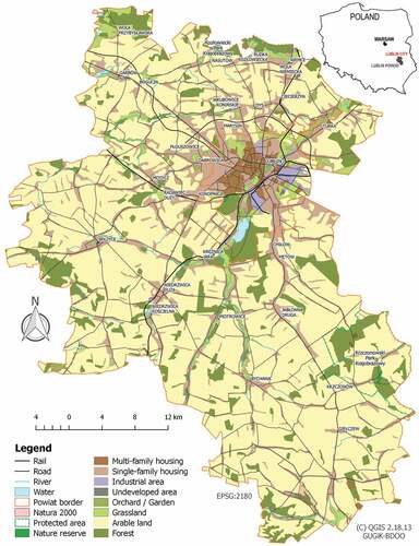
The area of Lublin powiat is mostly used as arable land, 70.6%, with additional 3.5% of grassland and 0.3% under orchards (Table 1). In the Lublin city, the arable land, grassland, and characteristic of Polish cities allotment gardens, cover in total 30.5%. What is interesting, the percentage of forests within city limits and within over 11 times larger Lublin powiat is almost identical, ca. 11–12%. Zones inhabited by man with the single-family housing are spread over the entire area of Lublin powiat along the main transportation routes, where they occupy 14.1%, and comprise also ca. one-third of the Lublin city area. The majority of highly urbanised zones with multi-family housing and industrial zones is located within the Lublin city limits (Table 1, Figure 1).

Table 1. Land use/land cover in the studied area calculated with use of the vector data retrieved from GUGiK-BDOO (2017)

Land use/land cover	City of Lublin (%)	Lublin powiat (%)	Studied area (average for both powiats) (%)
Arable land	14.8	70.6	66.1
Forest	12.2	11.2	11.3
Grassland	14.5	3.5	4.4
Allotment garden/Orchard	1.2/0	0/0.3	0.1/0.3
Single-family housing	31.1	14.1	15.5
Multi-family housing	16.3	0	1.1
Industrial and depot area	7.6	0	0.7
Water	2.0	0.1	0.3

The highest monthly average air temperatures are in July (17.2–18.3°C), and the lowest in January (from –3.2 to –4.5°C). The growing season with an average daily temperature of >5°C lasts on average around 206 days. The growing season usually begins in the first decade of April, and ends in the last decade of October. The average annual air temperature shows a slight decrease from 7.9 in the northwest to 6.8°C in the southeast (Kaszewski, Mrugała, & Warakomski, 1995). The amount of rainfall increases from 550 to 600 mm per year in the southwest direction. In the studied area, the average annual sunshine duration varies from 1518 in the west to 1675 h in the east, and the daily average is about 4.5 h. The average annual cloud cover is 61–68%. The cold period (November–February) is characterised by a large cloud cover, fairly uniform in terms of both size and spatial distribution. The warm period, on the contrary, is characterised by a much smaller but more varied cloud cover. Months with the smallest cloud cover are August and September (51–57%), and with the largest November and December (78–83%) (Kaszewski, Michalczyk, & Siwek, 2001). The average number of sunny days (below 20% cloud cover) ranges from 38 days in December to 50 days in August and September. The average number of cloudy days (over 80% cloud cover) varies from 140 days in August to 150 days in December.

Data sources and data processing

This study uses open access spatial and non-spatial data from diverse sources. Weather data for the Lublin-Radawiec weather station (No. 351220495; 51°13ʹ01ʺ N, 22°23ʹ37ʺ E, 240 m a.s.l.) for the period 1 March through 30 November 2017 and the long-term averages for the 1951–2016 were retrieved from the resources of Institute of Meteorology and Water Management – National Research Institute (IMGW–PIB, 2018); the data of the IMGW–PIB were processed. The General Geographic Database including: transport network, water, land cover, administrative units, localities and cities, and protected sites for the Lublin Voivodeship was obtained from Head Office of Geodesy and Cartography in Poland (GUGiK-BDOO, 2017; data last modified on 8 July 2016). Tree species in the forests of the studied area were identified on the basis of the Forest Data Bank of the Bureau for Forest Management and Geodesy (BULiGL-BDL, 2018). Crop types were found in GUS-BDL (2018) for territorial unit: Lubelskie Voivodeship, year 2016, category: Agriculture, Forestry and Hunting.

Given the size of the area studied and its localisation, we decided to analyse Landsat images so that we could process a limited number of scenes and obtain a homogenous cartographic results. Consequently for each study date only 1 or 2 scenes had to be selected (Table 2). Landsat 8 satellite images were derived from open access Landsat imagery archives at https://earthexplorer.usgs.gov/. The L1TP products were used, i.e. radiometrically calibrated and orthorectified using ground control points and digital elevation model data to correct for relief displacement; these were the highest quality Level-1 products suitable for pixel-level time series analysis. In the study, we applied the Landsat 8 images acquired between April and November of 2017 (Table 2). For the study the images from bands 5 (NIR, 845–885 nm) and 6 (SWIR, 1560–1660 nm) of the Landsat 8 Operational Land Imager sensor (OLI) working with the 30-meter spatial resolution were utilised (Irons, Dwyer, & Barsi, 2012; Mishra, Helder, Barsi, & Markham, 2016). The retrieved scenes were characterised with diverse cloud cover, and several dates were not available since the clouds covered the entire studied area. Consequently, only the best possible images were selected for the study. The pixels contaminated by clouds and cloud shadows were masked (Table 2) with white colour on the maps presenting spatial distribution of NDII and excluded from measurements with use of the quality image QB.tif available in the data package retrieved from Landsat archive (United States Geological Survey [USGS], 2016). All the spatial data were processed and the maps were prepared with QGIS 2.18.13, a free and open source GIS program (https://qgis.org/en/site/). All maps were presented in the projection system EPSG:2180.

Table 2. Images used in the study. Images courtesy of the U.S. geological survey

Acquisition date	Landsat product identifier	Masked area (%)
5 April 2017	LC08_L1TP_187024_20170405_20170414_01_T1	0.19
21 April 2017	LC08_L1TP_187024_20170421_20170501_01_T1	16.32
16 May 2017	LC08_L1TP_186024_20170516_20170525_01_T1 LC08_L1TP_186025_20170516_20170525_01_T1	27.41
1 June 2017	LC08_L1TP_186024_20170601_20170615_01_T1 LC08_L1TP_186025_20170601_20170615_01_T1	23.55
10 July 2017	LC08_L1TP_187024_20170710_20170725_01_T1	46.55
4 August 2017	LC08_L1TP_186024_20170804_20170812_01_T1 LC08_L1TP_186025_20170804_20170812_01_T1	11.40
11 August 2017	LC08_L1TP_187024_20170811_20170824_01_T1	0.00
27 August 2017	LC08_L1TP_187024_20170827_20170914_01_T1	7.79
28 September 2017	LC08_L1TP_187024_20170928_20171013_01_T1	0.35
24 November 2017	LC08_L1TP_186024_20171124_20171206_01_T2 LC08_L1TP_186025_20171124_20171206_01_T1	8.73

NDII images were obtained on the basis of band 5 and 6 Landsat 8 OLI images with “Raster calculator” function of QGIS. The Normalised Difference Infrared Index was computed as NDII = (NIR–SWIR)/(NIR+SWIR) or NDII = (ρ₈₆₅–ρ₁₆₁₀)/(ρ₈₆₅+ρ₁₆₁₀), where ρ₈₆₅ is the reflectance of a near-IR channel around 865 nm, and ρ₁₆₁₀ the reflectance of a shortwave-IR channel around 1610 nm. On the basis of the obtained NDII images, the relative distributions of NDII in the range from –1 to 1 in the 0.1-wide classes were calculated with a QGIS plug-in “Raster Pixel Count By ClassBreak” (https://plugins.qgis.org/plugins/RasterPixelCountStat/). Next, the area of pixels in each NDII class was divided by the total area of land not covered by clouds or their shadows, i.e. unmasked. The NDII distributions for each date were then checked for equality by way of the λ Kolmogorov–Smirnov test at P < 0.01. The linear regressions (n = 10) were calculated to search for relationships between NDII and weather conditions.

Results and discussion

Weather

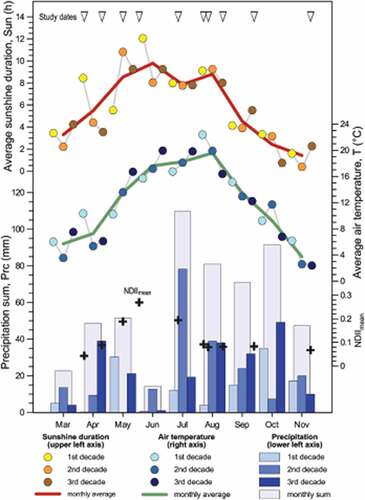
Weather conditions during the studied season are shown in Figure 2. The observed values deviated from the long-term average for this area for the years 1951–2016 (IMGW-PIB, 2018). Less precipitation was observed in March and May, and June was particularly dry with the precipitation reaching only ca. 20% of the long-term average. The remaining part of the growing season was wetter. In April, July, August, September, and November there were 20–40% more precipitation, and in October the rainfall was almost 2.5 times higher than in the years 1951–2016. In general, the studied growing season was warmer in comparison to the long-term average. In June, August, September, October, and November, the average monthly temperature was about 0.6–2°C higher. March was particularly warm, for which the average temperature exceeded the long-term average by 3.8°C. May and July were similar to the corresponding months in the years 1951–2016 and April was colder by 0.7°C. To conclude, March was warmer and drier than in the years 1951–2016, and afterwards there was cold and wet April. The end of spring was drier in comparison to the long-term average, followed by warm and wet summer and autumn.

Figure 2. NDII_mean and weather conditions during the experiment: average sunshine duration Sun (h), precipitation sum Prc (mm), and average air temperature T (°C)

Temporal trends of NDII

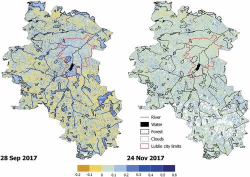
During the growing season NDII ranged from –0.2 to 0.6 (Table 3). The lowest NDII_max was noted on 24 November. On the 5 April, 11 August, and 28 September it was only slightly higher. The highest NDII_max was observed on the 1st of June. The NDII values covered the broadest range, 0.7, on 21 April, 1 June, 27 August, and the narrowest, 0.4, on the 24 November.

Table 3. Characteristics derived from the NDII distributions (minimum, maximum, and mean) and weather conditions within n days (n = 10, 20, 30) before NDII measurement: T_n – average air temperature (°C); Sun_n – average sunshine duration (h); Prc_n – precipitation sum (mm)

Date	NDIImin	NDIImax	NDIImean	T10	T20	T30	Sun10	Sun20	Sun30	Prc10	Prc20	Prc30
5 Apr	–0.2	0.4	0.043	10.2	7.6	6.5	7.8	5.1	4.0	0.1	16.7	22.5
21 Apr	–0.2	0.5	0.089	5.4	7.9	7.7	4.4	6.4	5.8	9.4	9.7	13.7
16 May	–0.1	0.5	0.189	10.9	9.7	8.1	7.5	5.2	5.4	12.0	68.4	69.6
1 June	–0.1	0.6	0.270	16.6	15.5	13.8	9.3	10.0	8.7	21.2	21.2	51.4
10 July	–0.1	0.5	0.194	16.7	18.4	17.9	7.9	8.7	8.4	12.2	13.2	25.9
4 Aug	–0.1	0.5	0.092	21.4	20.3	19.5	9.4	8.4	8.4	11.2	57.4	108.6
11 Aug	–0.1	0.4	0.080	22.4	21.3	20.2	9.1	8.6	8.3	4.0	14.2	88.4
27 Aug	–0.2	0.5	0.082	17.8	18.7	20.0	7.5	8.7	8.9	77.0	77.0	82.2
28 Sep	–0.2	0.4	0.083	13.0	14.5	14.7	4.0	4.6	4.5	41.0	56.0	71.0
24 Nov	–0.1	0.3	0.067	2.2	3.8	4.6	0.5	1.2	1.1	6.2	22.4	75.0

In the studied period NDII_mean initially increased to 0.270, then it decreased reaching a plateau value of around 0.08, and finally it dropped to 0.067 for the last examined date (Figure 2). The function of NDII_mean versus time followed a characteristic shape usually observed in the growing season. NDII was calculated with use of SWIR band which was sensitive to water content and biomass and therefore grew as vegetation coverage increased. Delbart et al. (2005) stated that NDII rose during leaf development; the moment at which NDII started increasing corresponded to the onset of greening up. After reaching the first peak value in the NDII function, the NDII curve could have diverse shape. As stated by Gu et al. (2007), it depended on weather conditions during the summer months. For drier years, the decrease of NDII was approximately twice as large in comparison to wetter years. At the end of the growing season, NDII decrease resulted from the vegetation colouring during autumnal senescence (Delbart et al., 2005).

Figure 3 shows the proportion of area with a specific NDII value in the studied powiats with respect to the unmasked part. During the growing season, the relative areas in each NDII class were varied. The size of relative area for which NDII exceeded 0 was increasing gradually until 10 July. The quantitative NDII distributions for August were very similar to each other which was confirmed with the statistical test. The same situation was observed for the NDII spatial distributions, presented in maps for 4, 11, and 27 August in Figure 4. The results (Figure 3) indicated a relatively stable vegetation state, which in August had reached its maturity. The quantitative NDII distributions for 21 April and 28 September were comparable, although the spatial distributions were quite different. For the two dates the main differences could be attributed to dissimilar state of the vegetation in the forest areas and in the arable land, since these two dates represented opposite stages of vegetation development characteristic of early spring and early autumn. On 24 November the studied area was the least varied in terms of the NDII value, both quantitatively and spatially; nearly 80% of the area was characterised by NDII in the range from 0 to 0.1 (compare Figures 3 and 4). The relatively high fraction of the area with NDII_0–0.1 in spring and in autumn could reflect a low coverage with vegetation being in its early or late stages of growth. The bare soil reflectance is higher for the SWIR band and lower for the NIR band than the respective reflectance of the pure green vegetation. As a result, NDII of a soil partially covered with vegetation is lower than that of the pure vegetation. In summer, the soil effect significantly decreases because of the dense vegetation cover (Huang, Chen, & Cosh, 2009).

Figure 3. The NDII relative distributions. The distributions marked by similar letters were not significantly different according to the λ Kolmogorov–Smirnov test at P < 0.01

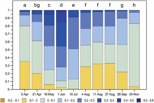
Figure 4. Normalised Difference Infrared Index, NDII, during the vegetation season 2017

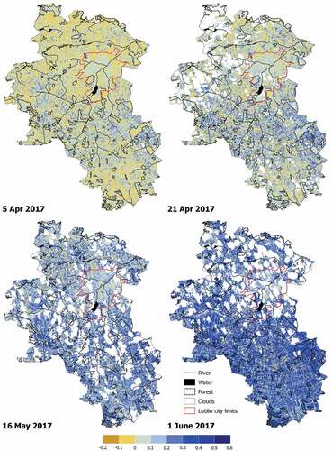
Figure 4. Continued

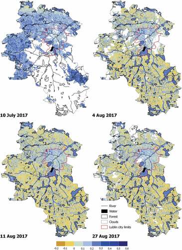
Figure 4. Continued

Spatial distribution of NDII in rural area

As stated before, ca. 70% of the Lublin powiat area was used as arable land (Figure 1), with cereals as the main crops including wheat Triticum aestivum L. (over 40% of cereals), triticale Triticosecale Wittm. ex A.Camus, barley Hordeum vulgare L., cereal mixtures, oats Avena sativa L., and rye Secale cereale L. (GUS-BDL, 2018). The maps (Figure 4) clearly showed the diversity of the arable land with respect to the NDII values on each studied date and during the vegetation season. On 5 April, a system of regular fields, denoted with blue colour, was clearly visible, where winter cereals grew, initially mainly in the middle part of the powiat and then in the remaining area. The maximum NDII values within agricultural land were noted on the 1 June. Then NDII in this area decreased gradually with the development and maturation of cereals and dropped below 0 in August. Low water content, particularly just before harvest, is a characteristic feature of cereals, hence the low NDII values. As stated by Gao (1996), the values of NDII for dry vegetation were negative. Moreover, the negative NDII values were expected for most bare soils, e.g. for the land after harvest, because reflectance in SWIR for wet and dry soils were usually greater than those in NIR region (Gao, 1996; Lobell & Asner, 2002). After the harvest of cereals, in some of the fields aftercrops were introduced and they were in early development phase in September. It resulted in NDII increase over 0 at the expense of area for which NDII was previously negative.

In forests in the Lublin powiat the dominating tree species were oak Quercus robur L. and Quercus petraea (Matt.) Liebl., and Scots pine Pinus sylvestris L., 40–50% for both oak and pine, with birch Betula pendula Roth, alder Alnus glutinosa (L.) Gaertn., hornbeam Carpinus betulus L., and beech Fagus sylvatica L. (BULiGL-BDL, 2018). The NDII variations for forest pixels showed a different behaviour compared to agricultural land. In forest areas on 5 April NDII exceeded 0.1 only for coniferous stands, while for broadleaved deciduous ones it was negative. With the emergence and development of leaves in the deciduous stands, NDII was gradually increasing. On 1 June, the NDII values in all forest areas achieved the maximum for the vegetation season approaching 0.3, and then they remained in the range 0.2–0.3 until the end of August. Comparable trends were observed by Bochenek, Ziolkowski, Bartold, Orlowska, and Ochtyra (2018). NDII decreased subsequently during the vegetation colouring at senescence, which was clearly visible in the maps for 28 September and 24 November. Forest areas, unlike arable land, were characterised by a lower dynamics of the NDII changes through the summer.

In permanent grassland, particularly in this located along river valleys, a similar situation occurred. The NDII values were relatively stable and confined in a fairly narrow range of 0.2–0.3 from May until the end of August, with the maximum above 0.3 on 1 June.

Spatial distribution of NDII in urban area

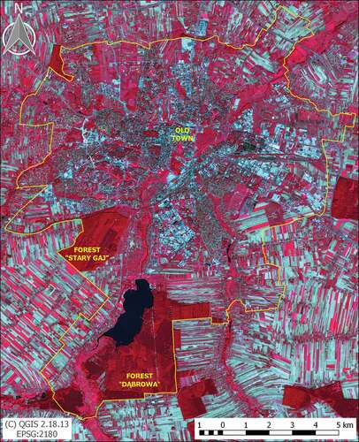
In the city of Lublin, the areas with vegetation cover comprise mostly forests, grassland, arable land, and also parks, green areas, cemeteries, gardens, and vegetation along transportation routes (Table 1). The forests “Stary Gaj” and “Dąbrowa” are located, respectively, in the western and southern parts of the city (Figure 5). “Dąbrowa” is a deciduous and a mixed forest with a large coniferous share. Forest composition is dominated by Scots pine and oak Quercus robur L., with admixtures of birch, alder, aspen Populus tremula L., hornbeam, and European larch Larix decidua Mill. “Stary Gaj” is a mixed forest with a coniferous share. In its composition oak Quercus robur L. and Scots pine prevail, with the addition of birch, hornbeam, small-leaved lime Tilia cordata Mill., and aspen. In forest areas in the city of Lublin, the temporal trends of the NDII were comparable to the changes detected in the Lublin powiat, which were described in detail in the previous section.

Figure 5. Sentinel-2 8–4–3 (NIR-R-G) false colour composite for the Lublin city area (yellow line) from the sentinel-2A MSI level-2A product acquired on 9 September 2017 (Product name: S2A_MSIL2A_20170909T093031_N0205_R136_T34UFB_20170909T093604.SAFE, courtesy of ESA)

Parks in Lublin cover 0.8% of the city area and they are unevenly distributed within a densely populated multi-family housing area. All parks have a deciduous tree stand. In the northwest part of Lublin city, there are grassland and xerothermic thickets. Other grassland is situated along river valleys and in recreational areas.

In April, grassland and arable land in the north of Lublin were characterised by the NDII values from –0.1 to 0, and locally below –0.1. During the growing season, NDII increased gradually reaching in selected areas a maximum of 0.3–0.4 on 10 July. The grassland and arable land showed a large spatial variation of the NDII values in the 0–0.4 range, visible in Figure 4 as a multi-coloured pattern. In August, the NDII values of 0.1–0.3 were observed on grassland, while within cultivated area a significant decrease of NDII due to crop maturation was visible. This trend of NDII was similar to the changes observed in the Lublin powiat. In September a further decrease of NDII occurred: to 0.1–0.2 in the grassland and below 0.1 in the arable land. On 24 November NDII in the above-mentioned areas was in the range of 0–0.1.

The area within the city of Lublin used as a single- and multi-family housing was characterised by specific features. This part of the city showed the highest heterogeneity in relation to the spatial resolution of the satellite sensor (Rashed, Weeks, Gadalla, & Hill, 2001). Urban land surface objects, e.g. buildings/roofs, roads, have a small spatial extent (Herold & Roberts, 2010) and the minimal spatial resolution recommended for their accurate spatial representation is 5 m (Albizua, Donezar, & Ibáñez, 2012; Jensen & Cowen, 1999). The urban environments possess also a high spectral heterogeneity resulting from a large diversity of land covers, such as vegetation, soil, anthropogenic features, etc., which also reveal the high degree of within-class spectral variability due to, e.g. geometry, condition, and age (Herold & Roberts, 2010; Kotthaus, Smith, Wooster, & Grimmond, 2014). Consequently, with use of medium spatial resolution images provided by Landsat 8, spectral mixing in the pixels is inevitable.

Based on a spectral library (Herold, Gardner, & Roberts, 2003), we evaluated the NDII_mean values of several human-made urban cover types typical of Lublin city area: brown composite shingle roof −0.07 ± 0.03; orange composite shingle roof 0.01 ± 0.03; brown metal roof 0.02 ± 0.04; light grey asphalt roof −0.05 ± 0.02; red tile roof −0.21 ± 0.09; light asphalt road −0.10 ± 0.02; dark asphalt and concrete roads 0.00 ± 0.05; parking lot −0.02 ± 0.12; railroad tracks −0.10 ± 0.02. To conclude, NDII for all of the mentioned cover types was below 0.1, which determined the NDII pattern within Lublin city.

In a single- and multi-family housing area on 5 April, NDII ranged from –0.1 to 0.2, with dominating values of 0–0.1 (Figure 4). In the maps a pattern of small blue patches (NDII 0.1–0.2) indicated urban greenery, which was scattered in a densely built-up area. Then, the area characterised by NDII over 0.1 was virtually stable from 21 April until 28 September, however in the course of the vegetation development the share of NDII over 0.2 fluctuated. In the Old Town of Lublin (Figure 5) where sealed human-made surfaces dominated, NDII was below 0.1 throughout the studied period. Taking into account the small variability of the limits of the land cover types in the most densely populated areas of Lublin city, the NDII values resulted mostly from the status of the vegetation during the growing season and its fraction within each pixel.

In the industrial area, NDII did not change strongly in the growing season, and its values were in the range 0–0.1 (Figure 4). A pattern of rectangular areas with a negative NDII was visible, reflecting the layout of industrial facilities. Small areas of urban greenery were discernible among industrial buildings as narrow stripes with NDII of 0.1–0.2. On 24 November, NDII in the residential and industrial areas was in the range of 0–0.1, similarly as stated for the forests, grassland, and arable land.

Relationships between NDII and weather conditions

The development of the vegetation canopy during the vegetation season was related to sunshine and temperature. NDII_mean, NDII_0.1–0.2, and NDII_0.2–0.3 strongly correlated with average sunshine duration and average air temperature within 10, 20, and 30 days before study dates (Tables 3 and 4). The area for which NDII was in the range from –0.1 to 0 increased in the period 5 April–24 November with the increase of temperature and sunshine duration within 10, 20, and 30 days before study dates. It was associated with the maturation in August of cultivated plants, mostly cereals, occupying a significant part of the studied area. The correlations of NDII_−0.1–0 with the average temperature and sunshine duration were even clearer when two parts of the growing season were considered. For dates 4 August–24 November these correlations were strong and positive; correlation coefficient R² was in the range of 0.957–0.990 at P < 0.0004. For the period 5 April–10 July, on the contrary, R² values were not statistically significant, with P in the range of 0.075–0.534.

Table 4. Linear regression equations of NDII vs. weather data: NDII_mean – mean NDII; NDII_f – fraction of area with respective NDII value, f = −0.1–0, 0–0.1, 0.1–0.2, 0.2–0.3, 0.3–0.4; T_n – average air temperature, Sun_n – average sunshine duration, and Prc_n – precipitation sum within n days (n = 10, 20, 30) before NDII measurement

Single linear regression equations	R^2	P
NDIImean = 0.0076 T10**	0.655	0.0016
NDIImean = 0.0077 T20**	0.666	0.0013
NDIImean = 0.0077 T30**	0.629	0.0022
NDII−0.1–0 = 0.0124 T10**	0.646	0.0018
NDII−0.1–0 = 0.0123 T20**	0.628	0.0022
NDII−0.1–0 = 0.0128 T30**	0.636	0.0020
NDII0.1–0.2 = 0.0146 T10***	0.764	0.0003
NDII0.1–0.2 = 0.0151 T20***	0.817	0.0001
NDII0.1–0.2 = 0.0151 T30***	0.812	0.0001
NDII0.2–0.3 = 0.0123 T10***	0.782	0.0002
NDII0.2–0.3 = 0.0125 T20***	0.800	0.0001
NDII0.2–0.3 = 0.0127 T30***	0.775	0.0002
NDIImean = 0.0166 Sun10***	0.742	0.0004
NDIImean = 0.0172 Sun20***	0.776	0.0002
NDIImean = 0.0178 Sun30***	0.760	0.0003
NDII−0.1–0 = 0.0253 Sun10**	0.624	0.0023
NDII−0.1–0 = 0.0250 Sun20**	0.585	0.0037
NDII−0.1–0 = 0.0263 Sun30**	0.587	0.0036
NDII0–0.1 = 0.7095*** – 0.0581 Sun10**	0.634	0.0036
NDII0–0.1 = 0.7505*** – 0.0647 Sun20**	0.692	0.0017
NDII0–0.1 = 0.7396*** – 0.0664 Sun30**	0.697	0.0016
NDII0.1–0.2 = 0.0301 Sun10***	0.763	0.0007
NDII0.1–0.2 = 0.0312 Sun20***	0.804	0.0001
NDII0.1–0.2 = 0.0330 Sun30***	0.818	0.0001
NDII0.2–0.3 = 0.0258 Sun10***	0.805	0.0001
NDII0.2–0.3 = 0.0266 Sun20***	0.833	0.0001
NDII0.2–0.3 = 0.0281 Sun30***	0.848	0.0001
NDIImean = 0.0015 Prc30**	0.498	0.0091
NDII0–0.1 = 0.0042 Prc30**	0.546	0.0057
NDII0.2–0.3 = 0.0023 Prc30**	0.530	0.0067

**P < 0.01; ***P < 0.001.

The relationship of NDII_mean, NDII_0–0.1, NDII_0.2–0.3 in the entire studied growing season with precipitation expressed as Prc₃₀, was weaker than with the above-mentioned weather parameters, and the regression coefficients did not exceed 0.55. Once again we examined the links between NDII and precipitation, considering separately the initial part of the growing season, 5 April–10 July, when the plants show the fastest development, and the second part, 4 August–24 November, during which plant maturation and senescence occur and the plants have significantly lower water requirements (Table 3). We stated that in the first part of the vegetation season NDII_mean correlated strongly and positively with the precipitation within 10 (Prc₁₀: R² = 0.960, P = 0.0004), and 30 (Prc₃₀: R² = 0.811, P = 0.0090) days before study dates. The strong NDII_mean – Prc₁₀ relationship resulted from the immediate response of the vegetation, mostly cereals that grew fast as the rain occurred (Chandrasekar et al., 2010). Starting from 4 August, similarly strong and positive relationship was observed only for Prc₃₀ (R² = 0.984, P = 0.0001). No significant correlations were found between NDII_0–0.1 and precipitation for any of the considered parts of the growing season. However, NDII_0.1–0.2 and NDII_0.2–0.3 quite clearly positively correlated with Prc₃₀ between 4 August and 24 November; R² equalled 0.855 for both NDIIs at P = 0.0053.

Summary and conclusion

In the present paper, the results of a preliminary study of the NDII applicability for monitoring of a heterogeneous rural and urban area during a growing season were shown. We evaluated the spatial and quantitative distributions, and temporal trends of NDII over a typical medium-sized European city with its surroundings. Vegetation was the component of land cover that was changing to the highest degree during the growing season. The NDII values over the vegetation areas covered a broad range from –0.1 to 0.6, which allowed for differentiation between vegetation ranges of various type, condition, and growth stage. The most dynamic temporal alterations of the NDII values were recorded within the arable land. In forest areas and grassland, on the other hand, the NDII values were relatively stable through the summer. It was associated with different life cycles of crops compared with vegetation of forests and permanent meadows. The NDII values were stable also in the built-up area in view of the practically constant state of human-made covers in the studied period.

NDII which reflected the condition of the vegetation, related to weather parameters during the growing season. NDII_mean, NDII_0.1–0.2, and NDII_0.2–0.3, associated with the canopy development and growth, were positively correlated with temperature and sunshine duration in the entire studied period. Similarly, NDII_−0.1–0 correlated positively with the average temperature and sunshine duration, however only from August when maturation over arable land began, until the end of November. For this part of the growing season, correlations between NDII and precipitation were also found. NDII_0.1–0.2 and NDII_0.2–0.3 positively correlated with precipitation within 30 days before study dates that could be useful in predicting the success with aftercrops. On the other hand, particularly high correlation between NDII_mean and precipitation within 10 days before study dates was noted in the first part of the vegetation season (April–July). It should be pointed out that stronger correlations were found when two separate parts of the growing season were considered. These specific intervals were associated with main phases of vegetation development, respectively, its rapid growth, and maturation and senescence, in which plants had diverse water requirements. It allows for more detailed monitoring the vegetation biomass with regard to weather conditions and applying treatments to mitigate the effects of possible water deficit.

Our research revealed that NDII could support a regular monitoring of LCLU in the urban and rural areas. However, homogenising of the NDII values after the growing season, as seen in the November map, implied that for this purpose only images of fully developed plant cover were suitable. In the climatic zone studied, the most appropriate might be the June, July, and August satellite imagery. In view of the fact that NDII is sensitive to plant water content, spatial and temporal distributions of the NDII index can support local authorities in land management and land use planning decisions especially with regard to use of water resources, and monitoring of agricultural productivity and crop maturity, drought, and hazard of fire. In addition, the found relationships between NDII and precipitation, temperature, and sunshine duration, could facilitate risk assessment and planning of agronomic practices in regard to the weather. Basing on these initial results, we plan to carry out analogous research for other growing seasons, in particular for those characterised by dissimilar weather conditions. The multi-year data will allow for comparisons and interpreting the results in a broader context. They also will provide the possibility to validate the correlations observed in the current study between NDII and selected weather conditions.

To support efficient land management, it is beneficial to increase the number of images available for growing season. The methodology described in this paper using Landsat 8 imagery is fully transferable to Sentinel-2 mission. The Sentinel-2 satellites provide continuity of Landsat image data, supplementing free and open-access repository of geodata. In addition, a high temporal resolution of Sentinel-2 with a revisit frequency of 5 days improves the chance for cloud-free images. The Sentinel-2A and Sentinel-2B collect images in 13 spectral bands including band 8a at 865 nm in the NIR and band 11 at 1610 nm in the SWIR. It is therefore possible to analyse urban and rural areas through the NDII index with the use of both data sources for prompt detection of changes in the environment.

Geolocation information

The area of interest was delimited by the latitudes of 50.852120 and 51.414809°N, and the longitudes of 22.098263 and 22.850314°E (EPSG:4326)/latitudes of 336,262.79 and 401,279.50 m, and the longitudes of 718,007.26 and 767,633.80 m (EPSG:2180).

Disclosure statement

No potential conflict of interest was reported by the authors.

References

- Albizua, L., Donezar, U., & Ibáñez, J.C. (2012). Monitoring urban development consolidation for regional management on water supply using remote sensing techniques. European Journal of Remote Sensing, 45, 283–292. doi:10.5721/EuJRS20124525
- Bochenek, Z., Ziolkowski, D., Bartold, M., Orlowska, K., & Ochtyra, A. (2018). Monitoring forest biodiversity and the impact of climate on forest environment using high-resolution satellite images. European Journal of Remote Sensing, 51, 166–181. doi:10.1080/22797254.2017.1414573
- BULiGL-BDL. (2018). Forest data bank, bureau for forest management and geodesy (https://www.bdl.lasy.gov.pl/portal/usluga-ogc-en)
- Chandrasekar, K., Sesha Sai, M.V.R., Roy, P.S., & Dwevedi, R.S. (2010). Land Surface Water Index (LSWI) response to rainfall and NDVI using the MODIS vegetation index product. International Journal of Remote Sensing, 31, 3987–4005. doi:10.1080/01431160802575653
- Delbart, N., Kergoat, L., Le Toan, T., Lhermitte, J., & Picard, G. (2005). Determination of phenological dates in boreal regions using normalized difference water index. Remote Sensing of Environment, 97, 26–38. doi:10.1016/j.rse.2005.03.011
- Dusseux, P., Vertès, F., Corpetti, T., Corgne, S., & Hubert-Moy, L. (2014). Agricultural practices in grasslands detected by spatial remote sensing. Environmental Monitoring Assessment, 186, 8249–8265. doi:10.1007/s10661-014-3973-5
- EDO-JRC (2011). NDWI: Normalized Difference Water Index. Product Fact Sheet: NDWI – Europe, Version 1, 1–6. Retrieved from http://edo.jrc.ec.europa.eu/documents/factsheets/factsheet_ndwi.pdf.
- Eurostat. (2014). Focus on European cities. In Eurostat regional yearbook 2014: Statistical books (pp. 287–304). Luxembourg: Publications Office of the European Union.
- Eurostat. (2016). Urban Europe Statistics on cities, towns and suburbs: Statistical books (pp. 1–286). Luxembourg: Publications Office of the European Union.
- Gao, B.-C. (1996). NDWI – A Normalized Difference Water Index for remote sensing of vegetation liquid water from space. Remote Sensing of Environment, 58, 257–266. doi:10.1016/S0034-4257(96)00067-3
- Gu, Y., Brown, J.F., Verdin, J.P., & Wardlow, B. (2007). A five-year analysis of MODIS NDVI and NDWI for grassland drought assessment over the central great plains of the United States. Geophysical Research Letters, 34, L06407. doi:10.1029/2006GL029127
- Gu, Y., Hunt, E., Wardlow, B., Basara, J.B., Brown, J.F., & Verdin, J.P. (2008). Evaluation of MODIS NDVI and NDWI for vegetation drought monitoring using Oklahoma Mesonet soil moisture data. Geophysical Research Letters, 35, L22401. doi:10.1029/2008GL035772
- GUGiK-BDOO. (2017). General geographic database, head office of geodesy and cartography in Poland (http://www.codgik.gov.pl/index.php/darmowe-dane/bdo250gis.html, http://mapy.geoportal.gov.pl/wss/service/ATOM/httpauth/atom/CODGIK_BDOO)
- GUS-BDL. (2018). Local data bank, central statistical office (https://bdl.stat.gov.pl/BDL/dane/teryt/jednostka)
- Han, Q., Luo, G., & Li, C. (2013). Remote sensing-based quantification of spatial variation in canopy phenology of four dominant tree species in Europe. Journal of Applied Remote Sensing, 7(1), 073485. doi:10.1117/1.JRS.7.073485
- Hardisky, M.A., Klemas, V., & Smart, R.M. (1983). The influences of soil salinity, growth form, and leaf moisture on the spectral reflectance of Spartina alterniflora canopies. Photogrammetric Engineering and Remote Sensing, 49(1), 77−83.
- Herold, M., & Roberts, D.A. (2010). The spectral dimension in urban remote sensing. In T. Rashed & C. Jürgens (Eds.), Remote sensing and digital image processing: Vol. 10. Remote sensing of urban and suburban areas (pp. 47–65)). Dordrecht: Springer Netherlands.
- Herold, M., Gardner, M., & Roberts, D.A. (2003). Spectral resolution requirements for mapping urban areas. IEEE Transactions on Geoscience and Remote Sensing, 41(9), 1907–1919. doi:10.1109/TGRS.2003.815238
- Huang, J., Chen, D., & Cosh, M.H. (2009). Sub-pixel reflectance unmixing in estimating vegetation water content and dry biomass of corn and soybeans cropland using normalized difference water index (NDWI) from satellites. International Journal of Remote Sensing, 30(8), 2075–2104. doi:10.1080/01431160802549245
- Huete, A.R. (1988). A soil-adjusted vegetation index (SAVI). Remote Sensing of Environment, 25, 295–309. doi:10.1016/0034-4257(88)90106-X
- Huete, A.R., & Justice, C. (1999). MODIS vegetation index (MOD13) algorithm theoretical basis document (Version 3). Retrieved from https://modis.gsfc.nasa.gov/data/atbd/atbd_mod13.pdf
- Hufkens, K., Friedl, M., Sonnentag, O., Braswell, B.H., Milliman, T., & Richardson, A.D. (2012). Linking near-surface and satellite remote sensing measurements of deciduous broadleaf forest phenology. Remote Sensing of Environment, 117, 307–321. doi:10.1016/j.rse.2011.10.006
- IMGW-PIB. (2018). Dane publiczne IMGW-PIB [Public data of IMGW-PIB] (https://dane.imgw.pl/data/dane_pomiarowo_obserwacyjne/dane_meteorologiczne/)
- Irons, J.R., Dwyer, J.L., & Barsi, J.A. (2012). The next landsat satellite: The landsat data continuity mission. Remote Sensing of Environment, 122, 11–21. doi:10.1016/j.rse.2011.08.026
- Jensen, J.R., & Cowen, D.C. (1999). Remote sensing of urban/suburban infrastructure and socio-economic attributes. Photogrammetric Engineering & Remote Sensing, 65(5), 611–622.
- Ji, L., Zhang, L., Wylie, B.K., & Rover, J. (2011). On the terminology of the spectral vegetation index (NIR − SWIR)/(NIR+SWIR). International Journal of Remote Sensing, 32(21), 6901–6909. doi:10.1080/01431161.2010.510811
- Jin, S., & Sader, S.A. (2005). MODIS time-series imagery for forest disturbance detection and quantification of patch size effects. Remote Sensing of Environment, 99, 462–470. doi:10.1016/j.rse.2005.09.017
- Kaszewski, B.M., Mrugała, S., & Warakomski, W. (1995). Temperatura powietrza i opady atmosferyczne na obszarze Lubelszczyzny (1951–1990) [Air temperature and precipitation in the Lublin region (1951–1990)]. In S. Uziak & R. Turski (Eds.), Środowisko przyrodnicze Lubelszczyzny. Klimat [Natural environment of the Lublin region. Climate] (pp. 1–71). Lublin, Poland: Lubelskie Towarzystwo Naukowe.
- Kaszewski, B.M., Michalczyk, Z., & Siwek, K. (2001). Klimatyczne uwarunkowania obiegu wody [Climatic conditions of the water cycle]. In Z. Michalczyk (Ed.), Badania Hydrograficzne w Poznawaniu Środowiska: Tom 6. Źródła Wyżyny Lubelskiej i Roztocza [hydrographic research in the studies of the environment: Vol. 6. Springs of the Lublin Upland and the Roztocze] (pp. 23–33). Lublin, Poland: Wydawnictwo UMCS.
- Kotthaus, S., Smith, T.E.L., Wooster, M.J., & Grimmond, C.S.B. (2014). Derivation of an urban materials spectral library through emittance and reflectance spectroscopy. ISPRS Journal of Photogrammetry and Remote Sensing, 94, 194–212. doi:10.1016/j.isprsjprs.2014.05.005
- Lobell, D.B., & Asner, G.P. (2002). Moisture effects on soil reflectance. Soil Science Society of America Journal, 66, 722–727. doi:10.2136/sssaj2002.7220
- Mishra, N., Helder, D., Barsi, J., & Markham, B. (2016). Continuous calibration improvement in solar reflective bands: Landsat 5 through landsat 8. Remote Sensing of Environment, 185, 7–15. doi:10.1016/j.rse.2016.07.032
- Nabielek, K., Hamers, D., & Evers, D. (2016). Cities in Europe. The Hague: PBL Netherlands Environmental Assessment Agency.
- Rashed, T., Weeks, J.R., Gadalla, M.S., & Hill, A. (2001). Revealing the anatomy of cities through spectral mixture analysis of multispectral imagery: A case study of the Greater Cairo region, Egypt. Geocarto International, 16(4), 5–16. doi:10.1080/10106040108542210
- USGS (2016). Landsat 8 (L8) data users handbook. Version 2.0. Retrieved from https://landsat.usgs.gov/sites/default/files/documents/Landsat8DataUsersHandbook.pdf.
- Wu, C., Gonsamo, A., Gough, C.M., Chen, J.M., & Xu, S. (2014). Modeling growing season phenology in North American forests using seasonal mean vegetation indices from MODIS. Remote Sensing of Environment, 147, 79–88. doi:10.1016/j.rse.2014.03.001
- Yilmaz, M.T., Hunt, E.R., Jr, & Jackson, T.J. (2008). Remote sensing of vegetation water content from equivalent water thickness using satellite imagery. Remote Sensing of Environment, 112, 2514–2522. doi:10.1016/j.rse.2007.11.014
- Zhang, X., Friedl, M.A., Schaaf, C.B., Strahler, A.H., Hodges, J.C.F., Gao, F., … Huete, A. (2003). Monitoring vegetation phenology using MODIS. Remote Sensing of Environment, 84, 471–475. doi:10.1016/S0034-4257(02)00135-9
- Zhang, X., Friedl, M.A., Schaaf, C.B., Strahler, A.H., & Schneider, A. (2004). The footprint of urban climates on vegetation phenology. Geophysical Research Letters, 31, L12209. doi:10.1029/2004GL020137
- Zhumanova, M., Mönnig, C., Hergarten, C., Darr, D., & Wrage-Mönnig, N. (2018). Assessment of vegetation degradation in mountainous pastures of the Western Tien-Shan, Kyrgyzstan, using eMODIS NDVI. Ecological Indicators, 95, 527–543. doi:10.1016/j.ecolind.2018.07.060