Effects of lidar coverage and field plot data numerosity on forest growing stock volume estimation

ABSTRACT

Forest parameter estimation is required to support the sustainable management of forest ecosystems. Currently, forest resource assessment is increasingly linked to auxiliary information obtained from remote sensing (RS) technologies. In forest parameter estimation, airborne laser scanning (ALS) data have been demonstrated to be an invaluable source of information. However, ALS data are often not available for the entire forest area, whereas images from multiple satellite systems offer new opportunities for large-scale forest surveys. This study aims to assess and estimate the contribution of field plot data and ALS data along with Landsat data to the precision of growing stock volume (GSV) estimates. We compared different approaches for model-assisted estimation of mean forest GSV per unit area using different proportions of field sample data, ALS cover data, and wall-to-wall Landsat data. Model-assisted estimators were used with NFI sample data in an Italian study area using 10 RS predictors, specifically the seven Landsat 7 ETM+ bands and three fine-resolution metrics based on ALS-derived canopy height. We found that relative to the standard simple expansion estimator, the model-assisted estimators produced relative efficiency of 1.16 when using only Landsat data and relative efficiencies as great as 1.33 when using increasing levels of ALS coverage.

KEYWORDS:

• Airborne laser scanning
• growing stock volume
• landsat 7 ETM+
• National Forest Inventory

Introduction

Forests play an important role in mitigating the effect of climate change and making recreation and economic contributions to our society. Worldwide, there is an increasing demand to improve forest parameter estimation in support of monitoring the state of these ecosystems. Usually, forest parameter estimates are provided by a design-based approach with field data collected in the frameworks of traditional national forest inventories (NFIs; Chirici et al., 2020; McRoberts et al., 2014; White et al., 2016). Estimates aggregated for large geographic areas are requested by national and international reporting frameworks such as Forest Europe and FAO (FAO, 2020; FOREST EUROPE, 2015). However, NFI data are expensive, since they require long and costly field campaigns, so a major scientific challenge is to develop new methods to produce useful forest information in a more cost-efficient way (Saarela et al., 2018; White et al., 2016). In recent decades, advancements in earth observation technologies have opened the possibilities for using remotely sensed (RS) data to support forest inventories, so that the strategies to collect information and produce forest inventory estimates have changed consequentially (Chirici et al., 2020; Kangas et al., 2018; Saarela et al., 2016; Waser et al., 2017; White et al., 2016). The exploitation of RS imagery became mandatory in deforestation and forest degradation surveys (REDD) because of the large cost of field surveys and forest inaccessibility in tropical and subtropical countries and remote areas (e.g., Corona et al., 2014; Pagliarella et al., 2016). RS data in combination with field data can be used to increase the precision of large-scale forest inventory estimates in two different stages: the design stage and the estimation stage or both (Saarela et al., 2018). At the design stage, RS data can be used for stratification (McRoberts et al., 2002) or probability sampling (Saarela et al., 2015; Lisańczuk et al., 2020). In the estimation stage, RS data can be used with either model-based inference (Gregoire, 1998; McRoberts et al., 2011) or design-based inference via stratified, post-stratified or model-assisted estimation (Särndal et al., 1992).

RS data can be acquired by different platforms, with different sensors, and at different resolutions, opening a vast array of methods useful for increasing the efficiency of forest parameter estimation (Holm et al., 2017; Puliti et al., 2018; Saarela et al., 2018; White et al., 2016). At the national inventory scale, methods based on satellite images are still the most widely used because of the small cost and temporally high frequency associated with acquisition of satellite imagery. The main disadvantages of using satellite imagery compared to airborne laser scanning (ALS) data, a form of light detection and ranging (lidar) data collected by airplane or helicopter platforms, are spatial accuracy and resolution, both of which are substantially greater for ALS. In fact, in recent years, many studies have successfully used ALS data to assist in the estimation of forest biophysical parameters, as well as to provide accurate and precise estimates of growing stock volume (GSV; Kotivuori et al., 2016; Montaghi et al., 2013; White et al., 2016). ALS has particularly revolutionized forest inventories with its great potential to produce three-dimensional (3D) forest vertical structure data for prediction of a variety of forest attributes (Hyyppä et al., 2008; Næsset, 2002; Næsset et al., 2004; Nilsson et al., 2017; Tompalski et al., 2019). Furthermore, high-performance computer servers represent a shift toward the possibility of detailed forest mapping, which can accurately identify individual tree crowns useful in support of forest management (Yun et al., 2021). However, ALS data are often limited by the cost of acquisition, processing, and data volume. As a result, complete ALS (or unmanned aerial vehicles) coverage is often impossible for large areas. Therefore, widespread and ready availability of such data is inhibited (Li et al., 2019; Puliti et al., 2018), in contrast to some RS data that are freely available wall-to-wall (e.g., satellite data).

Despite the well-documented use of wall-to-wall auxiliary data with model-assisted (Corona et al., 2014), the use of one wall-to-wall auxiliary dataset in conjunction with another auxiliary dataset with only partial coverage in a rigorous uncertainty assessment framework has been investigated in only a small number of recent papers (Gregoire et al., 2016; Puliti et al., 2018; Saarela et al., 2016, 2018). Holm et al. (2017) demonstrated how the hybrid 3-phase estimators can be used in situations where ALS data are used to relate ground plot measurements to lidar satellite observations (i.e., GLAS). Holm et al. (2017) further demonstrated that hybrid 3-phase estimators facilitate the assessment of mean biomass density and variance that account for sampling variability and the model prediction uncertainty associated with two predictive models (i.e., ground plot-ALS models and ALS-GLAS models). Saarela et al. (2016) illustrate a novel and design-based, model-assisted attempt to exploit wall-to-wall satellite information together with partial ALS information in the estimation of forest parameters from ground sample surveys.

The objective of this study is to assess the impact of partially available, fine resolution ALS data for model-assisted estimation of GSV. In particular, two main research questions are investigated.

• What is the effect of varying the ALS data forest coverage on GSV estimates?

• What is the effect of pseudo-plots constructed in the ALS stratum used to construct a GSV-RS model that is then applied to the entire study area?

To address these questions, we used an Italian dataset representing by forests with ALS data, covering the Alpine, and Mediterranean ecological regions, Landsat 7 ETM+ data, Canopy Height Model (CHM) derived ALS data, and NFI plots for which GSV was measured in the field.

Materials

Study area

The study was conducted in Italy (centered at 42° 30’ N and 12° 30’ E) in the forests for which ALS data are available, totaling 60,700 km² (D’Amico et al., 2021). The country is characterized by large vegetation variability due to its specific geographical and topographical conditions. The Italian peninsula has a typically flat coastal strip, a hilly part in the hinterland, and two main mountain ranges, the Alps in the north with peaks over 4800 m above sea level and the Apennines along the peninsula length.

Italian forests and other wooded lands are mainly distributed in hilly and mountainous areas covering 104,675 km², corresponding to 34% of the land area (INFC, 2004; Tabacchi et al., 2007). Italian forests consist mainly of broadleaf species (about 68% of the total). The most dominant tree species are Downy oak (Quercus pubescens), Pedunculated oak (Q. robur), Turkey oak (Q. cerris), Sessile oak (Q. petraea), European beech (Fagus sylvatica), each exceeding area of one million hectares. The most common coniferous forests, especially in the Alps, are those dominated by Norway spruce (Picea abies).

The Italian study area was tessellated into N = 97,116,385 square grid cells each with area of 530 m², equal to the NFI plot size (see, section 2.2.). The N grid cells constitute our target population U.

National forest inventory data

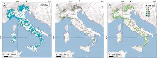
The Italian field reference data were measured in 2005 as part of the 2^nd Italian NFI (Figure 1 A; Chirici et al., 2020; INFC, 2004). Data for 2618 circular, 530-m² NFI field plots for which ALS data were acquired within five years of field measurement were available (Figure 1A). For each NFI plot, GSV (m³ ha⁻¹) for each callipered tree was predicted using species-specific allometric models developed by the NFI using tree DBH and tree height as independent variables (Tabacchi et al., 2011). The uncertainty of the allometric model predictions was considered negligible and ignored following previous results (McRoberts et al., 2016b, 2016a). The GSV of each NFI plot was predicted by aggregating volume predictions for all the trees callipered in the plot. Chirici et al. (2020) provides a complete description of GSV prediction for Italian NFI plots. The field plots selected are denoted as n elements of the population (U; Figure 2).

Remotely sensed data

Landsat predictors

A composite of Landsat 7 ETM+ images was computed using the Google Earth Engine (GEE) platform (Gorelick et al., 2017) which provides the complete, pre-processed archive of Landsat data. Specifically, we used the Landsat 7 Surface Reflectance Tier 1 images, i.e. atmospherically corrected and with the surface reflectance values calculated using the LEDAPS algorithm (Masek et al., 2013). We selected late-spring and summer images with less than 70% cloud cover (i.e. between April 1^st and September 30^th) acquired in 2005, the same period as the NFI field campaign. The image collection resulted in a total of 106 images. To avoid noise values in the images, pixels covered by clouds, shadow, water, and snow were masked using the CFMask algorithm implemented in GEE (Foga et al., 2017) and were not used to calculate the composite image. The composite image was constructed to obtain a unique image in specific time windows using all available satellite images (Wulder et al., 2019). The pixel values of the composite image are calculated as a function of the corresponding pixels of the acquired images in the time windows. In our case, the median function was used to calculate pixel values for each Landsat 7 band of the composite image (Figure 1 B).

Based on the Italian composite image, seven Landsat predictors were calculated, one for each Landsat band, specifically, the mean value of the composite image pixels within the plot area (Table 1). Moreover, the same Landsat predictors were calculated for all N grid cells of the Italian study area population.

Table 1. Landsat and CHM predictors

Data source	Variables name	Information
NFI	GSV	Field measured growing stock volume
Landsat 7 ETM+	Band 1	Blue	Wavelength 0.45–0.52 µm	Resolution 30 m
	Band 2	Green	Wavelength 0.52–0.60 µm	Resolution 30 m
	Band 3	Red	Wavelength 0.63–0.69 µm	Resolution 30 m
	Band 4	Near-infrared	Wavelength 0.77–0.90 µm	Resolution 30 m
	Band 5	Short-wave infrared	Wavelength 1.55–1.75 µm	Resolution 30 m
	Band 6	Thermal infrared	Wavelength 10.40–12.50 µm	Resolution 60 m
	Band 7	Short-wave infrared	Wavelength 2.09–2.35 µm	Resolution 30 m
CHM	CHM_Mean	Mean of 1 m × 1 m CHM pixels
	CHM_Prc90	90 percentile of 1 m × 1 m CHM pixels
	CHM_Std	Standard deviation of 1 m × 1 m CHM pixels

Canopy height model predictors

In Italy, a national raster grid CHM at 1 × 1 m resolution derived from available ALS data is available (D’Amico et al., 2021). Based on the national CHM (Figure 1C), three standard CHM variables were calculated for all available NFI plots and for the N study area grid cells. The CHM predictor variables were computed using the R-CRAN package “raster” (Hijmans & van Etten, 2012) and were the three height standard metrics: (i) the mean (CHM_Mean), (ii) the 90th percentile of the canopy height distribution (CHM_Prc90), and (iii) the standard deviation (CHM_Std), of the 1 × 1 m pixel values that were inside or intersected by the boundary of the 23 × 23 m pixels (Table 1). We used CHM because in Italy ALS point cloud data are not always available and because Chirici et al. (2016) has already demonstrated that GSV prediction accuracies are comparable for CHM metrics and point-based metrics. The CHM was derived from ALS datasets collected by different authorities between 2004 and 2017. The ALS datasets shared some common characteristics considered suitable for forestry applications (Goodwin et al., 2006; Wulder et al., 2008): acquisition flight altitudes between 500 m and 3000 m; spatial resolution of derived CHM ranging between 1 m and 5 m; pulse density between 0.4 and 5 pulses per m², which even at small values (0.4–1.0 pulses per m²) facilitate generation of reliable digital elevation models for plot-level forest estimates (~23 m pixel size – Jakubowski et al., 2013). However, several studies have demonstrated that a lag time greater than five years between field measurements and ALS data can be problematic when predicting forest variables (Wulder et al., 2008; Tompalski et al., 2019), especially when the area-based approach is used (Næsset, 2002). Thus, we selected CHM metrics derived from ALS acquired within five years of the NFI field survey. The grid cells for which the CHM metrics are available were denoted as the stratum₂ elements of the population (U; Figure 2).

Figure 1. A: Italian field plots; B: RGB Landsat composite image captured to create annual images with a median value for each pixel in ALS cover; C: Italian CHM cover.

Methods

Method overview

Full Landsat and CHM coverage, including for all NFI plots, were available for the study area. Our goal was to estimate the effects of varying the CHM and Landsat coverage proportions when estimating GSV.

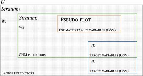
To evaluate the effects of varying CHM and Landsat coverages, we used a stratified estimation approach for which the strata were the Landsat coverage (stratum₁) and the CHM coverage (stratum₂), with proportions, respectively, denoted as w₁ and w₂ with w₁+w₂ = 1.

Estimates obtained using the simple expansion estimator, which is based exclusively on the NFI plot data within strata (Approach 0), were used for comparisons with estimates based on two additional approaches: (Approach 1) the model-assisted estimator within strata, and (Approach 2) the model-assisted estimator within strata using additional CHM-based pseudo-plots for model construction.

We progressively varied the amount of CHM and Landsat coverage using different w₁ and w₂ proportions (i.e., w₁ = 10% and w₂ = 90%; w₁ = 20% and w₂ = 80%; …; w₁ = 90% and w₂ = 10%). Based on the proportion, the CHM stratum was constructed by randomly selecting pixels until the correct proportion w₂ was achieved. All remaining pixels were then designated as the Landsat stratum. NFI plots were distributed between the two strata according to their locations. For each proportion, we repeated the three approaches iteratively, selecting randomly the strata 50 times. Finally, the average values over all iterations were used to estimate the effects of CHM coverage change among approaches (Tables A1, A2, A3).

For Approach 0 data for all plots were used with the simple expansion estimator. For Approach 1, the stratified estimators were used with the within-strata means and variances estimated using the model-assisted regression estimators. For Approach 2, we constructed pseudo-plots by using the CHM variable to predict GSV for some selected plot-size areas in the CHM stratum. The intent was to determine if the combination of the NFI plot data and the pseudo-plot predictions would produce a more accurate GSV-Landsat model. We then used stratified estimation for which within-strata means and variances were estimated using the model-assisted estimators using data for only the within-strata NFI plots but no pseudo-plots.

Figure 2. Predictors overview. The w₁ and w₂ proportions varied progressively.

NFI plot selection

In the temporal lag between NFI field plot measurement (2005) and ALS acquisition (D’Amico et al., 2021), some plots were harvested or otherwise substantially disturbed between the two dates. To alleviate this discrepancy, we selected ALS data acquired in a range of five years of the NFI field survey. Moreover, plots disturbed in the period between the laser scanning and the field inventory or incorrectly linked to the ALS data due to poor plot locations were identified and removed in the following way. A residual analysis was performed with a weighted estimation of heteroscedastic residual variances (section 3.3). Specifically, plots for which the ratio of the residual calculated as the difference between the observation and prediction and the corresponding residual standard deviation estimated through the weighted method were greater than 2.0 were considered outliers. In total, 3% of the NFI plots were identified as outliers and removed from the final dataset (2534 NFI plots).

Nonlinear power model

A nonlinear power regression model was used to describe the relationship between GSV for NFI plots and associated CHM metrics. The simple correlation coefficient between CHM metrics and GSV for stratum₂ (CHM) was performed to select the CHM metric that produced the most accurate predictions. The model has the mathematical form,

(1) $y_i={\beta }_1\ast {x_i}^{{\beta }_2}+{\epsilon }_i$(1)

where i index plots, $y_i$ is GSV, $x_i$ is the ALS metric, ${\epsilon }_i$ is a random residual, and the βs are parameters to be estimated. An advantage of this model is that when the ALS metrics are zero, as is the case for many non-forest plots, the prediction will also be zero. Preliminary analyses indicated that the individual ALS metric that produced the most accurate predictions was CHM_mean (Eq. (1)(1) $y_i={\beta }_1\ast {x_i}^{{\beta }_2}+{\epsilon }_i$(1) ). All possible combinations of one, two, and three additional independent variables together with CHM_mean were considered for the model. However, none contributed to statistically significantly increasing the quality of model fit to the data.

As with most biological data, residual heteroscedasticity in the form of greater residual variances for larger observations was evident. Although the mathematical form of Eq. (1)(1) $y_i={\beta }_1\ast {x_i}^{{\beta }_2}+{\epsilon }_i$(1) readily lends itself to a log transformation for either linearization or reduction of heteroscedasticity, weighted nonlinear least squares were used for these analyses. The heterogeneous model residual variance, ${\sigma }_i^2$, was characterized using a 5-step procedure (McRoberts et al., 2016b, Section 3.2.2): (i) calculate the model prediction residuals as ${\epsilon }_i=y_i-\hat{y}$ where ${\hat{y}}_i={\hat{\beta }}_1\ast x_1^{{\hat{\beta }}_2}$; (ii) order the pairs ($x_i$, ${\epsilon }_i$) to $x_i$; (iii) aggregate the ordered pairs into groups of size 25; (iv) for each group, g, calculate the mean, $\overline{x_g}$, of the predictor variable and the standard deviation, $\widehat{{\sigma }_g}$, of the grouped residuals; and (v) model the relationship between ${\hat{\sigma }}_g$ and ${\bar{x}}_g$ as,

(2) $\widehat{{\sigma }_g}=\lambda \ast {\bar{x}}_g+{\epsilon }_g,$(2)

where $\lambda$ is a model parameter estimated using ordinary least squares techniques. For the weighted nonlinear least squares technique, each observation was weighted inversely to its residual variance estimated by substituting the CHM mean for ${\bar{x}}_g$ in Eq. (2(2) $\widehat{{\sigma }_g}=\lambda \ast {\bar{x}}_g+{\epsilon }_g,$(2) ; McRoberts et al., 2018).

As for the CHM metric, in stratum₁ (non-CHM), a nonlinear power regression model was used to describe the relationship between GSV from NFI plots and associated Landsat metrics. To select the combination of independent variables that produced the greatest prediction accuracy, in addition to the seven Landsat predictors, we calculated the normalized difference for all the predictor combinations (21 new indices). A subset of the three Landsat predictors, with the greatest correlations to GSV observations, were selected to develop the model:

(3) $y_i={\beta }_3\ast {x_{ij}}^{{\beta }_4}\ast e^{{\beta }_5\ast x_{ij}+{\beta }_6\ast x_{ij}}+\epsilon$(3)

where i indicates plots or population units, $x_{ij}$ is the jth Landsat metric, ${\beta }_s$ are parameters to be estimated.

Stratified estimator (approach 0)

The essence of stratified estimation is to assign population units to groups or strata, where for this study the strata are the CHM coverage and the non-CHM (Landsat) coverage, estimate the within-strata sample plot means and variances using the simple expansion estimators, and then calculate the population estimate as a weighted average of the within-strata estimates where the weights are proportional to the stratum sizes. With stratified estimation, (1) the strata weights are calculated as the relative proportions of the population area corresponding to strata, and (2) the sample unit is assigned to a single stratum. For this study, we varied the strata proportions and consequently the strata weights. At the same time, we assigned NFI plots to strata based on the stratum assignment of the population units containing the plot centers.

Stratified estimates of means and variances are calculated using estimators provided by Cochran (1977) .

(4) ${\hat{\mu }}_{STR}=\sum _{h=1}^H{w}_h{\hat{\mu }}_h$(4)

(5) $\widehat{Var}({\hat{\mu }}_{STR})=\sum _{h=1}^H{w_h}^2\frac{{\hat{\sigma }}_h^2}{n_h}$(5)

where ${\hat{\mu }}_{STR}$ denotes the stratified estimator of the mean; h = 1, …, H denote strata; $w_h$ denotes the hth stratum weight; and $n_h$ denotes the number of plots assigned to the hth stratum;

(6) ${\hat{\mu }}_h=\frac{1}{n_h}\sum _{i=1}^{n_h}{y}_{hi}$(6)

denotes the sample mean for the hth stratum; $y_{hi}$ is the ith sample observation of GSV in the hth stratum; and

(7) ${{\hat{\sigma }}_h}^2=\frac{1}{n_h-1}\sum _{i=1}^{n_h}\left(y_{hi}-{\hat{\mu }}_h\right)$(7)

denotes the sample variance for the hth stratum.

The simple expansion estimator, used here within strata and sometimes referred to as “simple random sample” or “direct” estimator, has some advantages: (i) simplicity, using only the sample data, without fitting a model or some other statistical procedure, (ii) intuitiveness, using common arithmetic mean and the Central Limit Theorem to determine its variance; and (iii) unbiasedness under simple random and systematic sampling designs (Moser et al., 2017). The disadvantage of the simple expansion estimator is the possibly large variances, mainly when the sample size is small and/or the population is highly variable (McRoberts et al., 2013). Nevertheless, because it is unbiased, this approach was used to compare the different model-assisted estimators used with the different predictors and strata proportions.

Stratified estimation with model-assisted estimation within strata (approach 1)

Model-assisted estimators use models based on auxiliary data to enhance inferences but rely on probability samples for validity. For this study, within each stratum, we used the model-assisted regression estimators of means and variances provided by Särndal et al. (1992). The population and the corresponding plots are divided into two strata, sequentially changing their proportions (w₁ and w₂).

(8) ${\hat{\mu }}_1=\frac{1}{N_1}\sum _{i=1}^{N_1}{\hat{y}}_i^{Landsat}-\frac{1}{n_1}\sum _{i=1}^{n_1}\left({\hat{y}}_i^{Landsat}-y_i^{Landsat}\right)$(8)

(9) ${\hat{\mu }}_2=\frac{1}{N_2}\sum _{i=1}^{N_2}{\hat{y}}_i^{CHM}-\frac{1}{n_2}\sum _{i=1}^{n_2}\left({\hat{y}}_i^{CHM}-y_i^{CHM}\right)$(9)

where: N₁ is the number of Landsat pixels in the non-CHM stratum; N₂ is the number of CHM cells in the CHM stratum; $y_i^{Landsat}$ is an inventory plot observation from the non-CHM stratum; ${\hat{y}}_i^{Landsat}$ is a prediction from the GSV-Landsat model; $y_i^{CHM}$ is an inventory plot observation from the CHM stratum; ${\hat{y}}_i^{CHM}$ is a prediction from the GSV-CHM model. The estimate of the overall mean and standard error are:

(10) $\hat{\mu }=\sum _{h=1}^2{w}_h\cdot {\hat{\mu }}_h$(10)

and

(11) $SE\left(\hat{\mu }\right)=\sqrt{\widehat{Var}\left(\hat{\mu }\right)}=\sqrt{\sum _{h=1}^2{w}_h^2\cdot \frac{{\hat{\sigma }}_h^2}{n_h}}$(11)

where

(12) ${\hat{\sigma }}_1^2=\frac{1}{\left(n_1-1\right)}\sum _{i=1}^{n_1}{\left({\hat{y}}_i^{Landsat}-y_i^{Landsat}\right)}^2$(12)

and

(13) ${\hat{\sigma }}_2^2=\frac{1}{\left(n_2-1\right)}\sum _{i=1}^{n_2}{\left({\hat{y}}_i^{CHM}-y_i^{CHM}\right)}^2$(13)

The primary advantage of the model-assisted estimators is that they capitalize on the relationship between the sample observations and their model predictions to reduce the variance of the estimate of the within strata means and, by extension, the population mean (McRoberts et al., 2014).

Stratified estimation with model-assisted estimation within strata using pseudo-plots for model construction (approach 2)

For Approach 2, we added pseudo-plots to investigate the possibility of constructing a more accurate GSV-Landsat model. We first tessellated the study area into 8 × 8 km grid cells. In grid cells that had pixels selected for the CHM stratum, we randomly selected one pixel that was not already associated with an NFI plot. Pseudo-plots were constructed at the selected locations by using the power model (Eq. (1(1) $y_i={\beta }_1\ast {x_i}^{{\beta }_2}+{\epsilon }_i$(1) )) and the CHM variables to predict GSV. Based on the selection of pseudo-plot locations, the intensity of pseudo-plot sampling was proportional to the sampling intensity of NFI plots in the CHM stratum.

Based on the two strata sizes, and thus the number of NFI plots (n₂) in the CHM stratum, the GSV for the pseudo-plots was estimated. The inventory plots (n₁ + n₂) and the CHM-based pseudo-plots were used to construct a GSV-Landsat model that was applied to the entire study area. Next, the model-assisted estimator with NFI plots in the Landsat stratum (n₁) was used to estimate the mean GSV within it (stratum₁; Eq. (8)(8) ${\hat{\mu }}_1=\frac{1}{N_1}\sum _{i=1}^{N_1}{\hat{y}}_i^{Landsat}-\frac{1}{n_1}\sum _{i=1}^{n_1}\left({\hat{y}}_i^{Landsat}-y_i^{Landsat}\right)$(8) ). While for computing GSV estimates in the CHM stratum (stratum₂), presented NFI plots (n₂) are used. Thus, although pseudo-plots are also included in the CHM stratum, we used this same model to predict GSV for the entire CHM stratum for the model-assisted estimator. Consequently, pseudo-plot data do not affect model-assisted estimation so only NFI plots (n₂), were used to estimate the mean GSV within CHM stratum (stratum₂; Eq. (9)(9) ${\hat{\mu }}_2=\frac{1}{N_2}\sum _{i=1}^{N_2}{\hat{y}}_i^{CHM}-\frac{1}{n_2}\sum _{i=1}^{n_2}\left({\hat{y}}_i^{CHM}-y_i^{CHM}\right)$(9) ). The same effect occurred in calculating the variance and, consequently, the standard errors, which for the two strata were calculated as Eq. (11)(11) $SE\left(\hat{\mu }\right)=\sqrt{\widehat{Var}\left(\hat{\mu }\right)}=\sqrt{\sum _{h=1}^2{w}_h^2\cdot \frac{{\hat{\sigma }}_h^2}{n_h}}$(11) .

Also, in this approach, we varied the strata proportions and weights of population units in strata. While in the non-CHM stratum (stratum₁) there were the corresponding NFI plots, in the CHM one (stratum₂) there were NFI plots and pseudo-plots, both increased progressively, simulating greater CHM coverage. Particularly, the number of pseudo-plots increased as the size of the CHM stratum increased, up to a maximum of 567 pseudo-plots selected in the 23 × 23 grid (Table A3).

Relative efficiency

To assess the efficiency of the model-assisted estimators, we compared variance estimates obtained with each approach with variance estimates obtained with the simple expansion estimator, taken as reference, and calculated the relative efficiency coefficient (RE) as:

(14) $RE=\frac{\widehat{Var}\left({\hat{\mu }}_{SEE}\right)}{\widehat{Var}\left({\hat{\mu }}_s\right)}$(14)

where $\widehat{Var}\left({\hat{\mu }}_{SEE}\right)$ is the simple expansion estimator variance (Eq. (6(6) ${\hat{\mu }}_h=\frac{1}{n_h}\sum _{i=1}^{n_h}{y}_{hi}$(6) )), and $\widehat{Var}\left({\hat{\mu }}_s\right)$ is the variance for Approaches 1 and 2 with model-assisted estimation within strata.

Because RE is the ratio between the values of the variance of $\widehat{Var}\left({\hat{\mu }}_{SEE}\right)$ and $\widehat{Var}\left({\hat{\mu }}_s\right)$, values greater than 1 are evidence of greater precision for the model-assisted estimates (Moser et al., 2017). The RE coefficient can be interpreted as the factor by which the original sample size would have to be increased to achieve the same precision without using the remotely sensed auxiliary data as that achieved using the remotely sensed auxiliary data (Chirici et al., 2020; Francini et al., 2020; Francini et al., 2021).

Results and discussion

Nonlinear power model

The analysis of the simple correlation coefficient of Landsat metrics used as independent variables for predicting GSV in stratum₁ (non-CHM) and the simple correlation coefficient between the CHM metric and GSV for stratum₂ (CHM) are reported in Table 2. The final models for stratum₁ (Eq. (3(3) $y_i={\beta }_3\ast {x_{ij}}^{{\beta }_4}\ast e^{{\beta }_5\ast x_{ij}+{\beta }_6\ast x_{ij}}+\epsilon$(3) )) and stratum₂ (Eq. (1(1) $y_i={\beta }_1\ast {x_i}^{{\beta }_2}+{\epsilon }_i$(1) )) reported R² of 0.26 and 0.44, respectively (Figure 3).

Figure 3. GSV (m³ ha⁻¹) observation vs prediction scatters plot and residuals. On the top: CHM model prediction, on the bottom: Landsat model prediction. Darker dots are average of aggregations of 25 observations.

Table 2. Indices with the greatest correlation coefficients between the GSV and Landsat and CHM metrics

Metric	RMSE	R^2	MAE
B5_B6	128.03	0.224	94.37
SWIRI (Band5)	128.81	0.214	95.26
B6_B7	129.02	0.212	95.53
CHM_Mean	109.19	0.435	75.94

Stratified estimator with the simple expansion estimator within strata (approach 0)

The stratified estimator of the mean with the simple expansion estimator within strata yielded overall estimates of $\hat{\mu }$ = 159.58 m³ ha⁻¹ with $SE\left(\hat{\mu }\right)$ = 2.89 m³ ha⁻¹. Considering each stratum, the estimates of the mean ranged from ${\hat{\mu }}_1$=157.6 m³ ha⁻¹ to ${\hat{\mu }}_1$=160.4 m³ ha⁻¹, for stratum₁ and between ${\hat{\mu }}_2$ = 158.2 m³ ha⁻¹ and ${\hat{\mu }}_2$= 160.67 m³ ha⁻¹ for stratum₂. These differences are attributed to differences between strata weights and the proportions of plots assigned to strata (Table A1, Figure 5). In particular, stratum₁ standard errors, SE(${\hat{\mu }}_1)$, ranged approximately from 3.0 m³ ha⁻¹ to 9.1 m³ ha⁻¹ while stratum₂ standard errors, SE(${\hat{\mu }}_2)$, from 3.0 m³ ha⁻¹ to 9.1 m³ ha⁻¹ with the greatest estimates for small stratum proportions and the greatest estimates for large stratum proportions and numbers of plots.

Stratified estimation with model-assisted estimation within strata (Approach 1)

The model-assisted estimates of the mean for the entire population and for the individual strata based on different stratum proportions were similar to the corresponding simple expansion estimates obtained for Approach 0 with greater similarity for increasing stratum₂ (CHM) proportions (Table A2, Figure 5). The standard errors for estimates of the means were smaller with increasing stratum proportions, with values from $SE\left({\hat{\mu }}_1\right)$ = 2.5 m³ ha⁻¹ to $SE\left({\hat{\mu }}_1\right)$ = 7.8 m³ ha⁻¹ for stratum₁ and form $SE\left({\hat{\mu }}_2\right)$ = 2.2 m³ ha⁻¹ to $SE\left({\hat{\mu }}_2\right)$= 7.0 m³ ha⁻¹ for stratum₂. (Figure 4).

Figure 4. Standard error of the GSV estimate in Approach 1 overall and for both CHM and Landsat strata.

Similarly, the bias estimates for the MA estimator in both strata were smaller with increasing stratum proportions from ${\widehat{Bias}}_1$ = −1.7 m³ ha⁻¹ to ${\widehat{Bias}}_1$ = −1.9 m³ ha⁻¹ for stratum₁ and from ${\widehat{Bias}}_2$ = −0.4 m³ ha⁻¹ to ${\widehat{Bias}}_2$ = −5.4 m³ ha⁻¹ for stratum₂. Small bias estimates reflect the means of differences between GSV observations and model predictions, and small variance estimates can be attributed to the good quality of fit of the power model to the data. However, even with small bias estimates, ${\hat{\mu }}_1$ was underestimated for all stratum proportions. This spectral saturation effect with underpredictions for plots with GSV greater than 500 m³ ha⁻¹ is well documented in the literature (Chirici et al., 2020). Indeed, Landsat spectral reflectance values are not sensitive to multilayer canopy forests or dense forests (Zhao et al., 2016). Moreover, complex topographic features, such as for most of the Italian forest area, may affect the spectral signature and the data saturation values of forest aboveground biomass and GSV (Lu et al., 2016; Nichol & Sarker, 2011). The saturation effect, although less severe, has also been reported in the literature for ALS data (Giannetti et al., 2018; Lefsky et al., 2005; Nilsson et al., 2017).

Stratified estimation with model-assisted estimation within strata using pseudo-plots for model construction (Approach 2)

To construct a more accurate model for predicting GSV from the Landsat auxiliary data, we generated pseudo-plots using the CHM variable to predict GSV for selected areas in the CHM stratum. The model-assisted estimates of the means for the entire population and for the individual stratum based on different stratum proportions were similar to the means estimates for the preceding Approach 1 (Table A3, Figure 5). For the Landsat stratum₁, the bias estimates for the model-assisted estimator in the Landsat stratum were smaller than the estimates for Approach 1 for almost all proportions, with values from ${\widehat{Bias}}_1$ = 1.61 m³ ha⁻¹ to ${\widehat{Bias}}_1$ = −2.8 m³ ha⁻¹. The smaller values of ${\widehat{Bias}}_1$ for Approach 2 relative to those for Approach 1 reflect the positive influence of the pseudo-plots which neutralized the saturation effect of Landsat data. However, as the Landsat stratum size decreases and, therefore, with fewer NFI plots (n₁), ${\widehat{Bias}}_1$ tends to increase in absolute value. This inconsistent bias trend depends on the decreasing numbers of NFI plots, and also on the positive effect of increasing the numbers of pseudo-plots. For the Landsat stratum₁, the strata standard errors for estimates of the means were smaller for increasing stratum proportions with values ranging from $SE\left({\hat{\mu }}_1\right)$ = 2.6 m³ ha⁻¹ to $SE\left({\hat{\mu }}_1\right)$ = 7.9 m³ ha⁻¹ for stratum₁. In addition, the standard errors for estimates of the means were smaller with increasing numbers of pseudo-plots with values from $SE\left(\hat{\mu }\right)$ = 2.5 m³ ha⁻¹ to $SE\left(\hat{\mu }\right)$= 2.2 m³ ha⁻¹. For stratum₂, bias ${\widehat{Bias}}_2$ and $SE\left({\hat{\mu }}_2\right)$ were the same as for Approach 1.

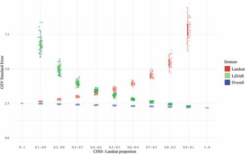
Figure 5. GSV and standard error of the estimated GSV distributions, for approaches 1 and 2 over 50 iterations for each strata proportion. The green dashed line represents the mean value of the simple expansion estimator (Approach 0).

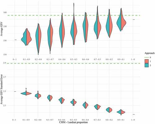
Relative Efficiency

Relative efficiency was calculated for each approach with estimates obtained with the simple expansion estimator as reference (Eq. (14(14) $RE=\frac{\widehat{Var}\left({\hat{\mu }}_{SEE}\right)}{\widehat{Var}\left({\hat{\mu }}_s\right)}$(14) ); Tables A1, A2, A3). RE (Eq. (14(14) $RE=\frac{\widehat{Var}\left({\hat{\mu }}_{SEE}\right)}{\widehat{Var}\left({\hat{\mu }}_s\right)}$(14) )) for the stratified estimation with model-assisted estimation within strata ranged between 1.17 and 1.31. For situations with 100% Landsat and 100% CHM, RE were, respectively, 1.16 and 1.33. For Approach 2, REs were between 1.17 and 1.31, with relevant implications for inventory applications. Indeed, given the considerable current expense associated with ground sampling, large REs have the potential to greatly enhance NFI estimation. However, the RE values obtained using pseudo-plots to construct a more accurate model-assisted estimator using the Landsat auxiliary data are comparable to those for Approach 1.

RE values for w₂ =0.5 are especially relevant for the various approaches examined, because with the release of data from the 3^rd NFI in coming months, approximately 50% of Italian forests will have ALS coverage. The 3^rd NFI field surveys have been carried out since 2017. So, unless a nationwide ALS survey is conducted in the short term to ensure the temporal consistency with the measured field plots, CHM coverage will continue to be characterized by only partial and fragmentary coverage. The method presented in this work may be applied operationally. It is worth noting that completion and updating of the national ALS data cover are planned for the following National Recovery and Resilience Plan (NRRP; ”MITE,” 2021).

RE for stratified estimation with model-assisted estimation within strata with equal strata proportions for Approach 1 produced RE =1.23. In Approach 2, with equal strata proportions, RE =1.23.

For both approaches, RE values were greater for greater CHM stratum proportions. Nevertheless, even with limited ALS cover, cost-efficiency should not be ignored. For example, RE = 1.234 (equal to 50% ALS coverage in Approach 1) means that to achieve the same precision levels without the use of the auxiliary information, sample sizes would have to be increased by a factor of 0.234, i.e., for this study, the sample size of 2534 would have to be increased by 0.234 × 2534 = 593 plots. For a 2021 measurement cost of approximately 500€/plot, the cost savings from using the auxiliary information and stratified estimation is a non-negligible amount of 296,500€.

Summary

The reasons that led to the development of this methodology are related to the historical Italian situation and the upcoming release of the 3^rd NFI data. Field surveys of the 3^rd inventory were performed between 2017 and 2020 (De Laurentis et al., 2021), and the time-consistent, available ALS data are fragmented and distributed over the whole territory. The approaches developed in this work are geared toward considering the availability of non-wall-to-wall ALS data and how their availability affects large-scale volume estimation (Figure 6).

The simple expansion estimator was used as a reference and then calculated for each stratum proportion, although, as expected, these changes provided comparable values for both strata (Table A1).

The stratified estimator with model-assisted estimation within strata produced more precise estimates (decrease in $\widehat{SE}\left(\hat{\mu }\right)$), as the CHM coverage increased (Table A2). Indeed, the use of ALS data confirms the potential to improve GSV estimation performance because of its well-known ability to capture canopy information (Lu et al., 2012). Of note was the underestimation for stratum₁ (Landsat). The Landsat estimation model (Eq. (3(3) $y_i={\beta }_3\ast {x_{ij}}^{{\beta }_4}\ast e^{{\beta }_5\ast x_{ij}+{\beta }_6\ast x_{ij}}+\epsilon$(3) )) produced small estimated model-assisted bias (${\widehat{Bias}}_1$= −2 m³ ha⁻¹), although the average GSV for the study area was ${\hat{\mu }}_1$ 154.9 m³ ha⁻¹, substantially less than the average observed plot GSV of 159.6 m³ ha⁻¹. This difference is ascribed to the saturation effect of the Landsat predictors in the GSV estimation. Uncertainties can be attributed to both typical coppices for complex forest structures and mature forests with volumes greater than 500 m³ ha⁻¹ that cannot be accurately predicted using data from passive optical sensors (Chirici et al., 2020; Lu et al., 2012). More accurate image composite methods such as the Best Available Pixel (BAP; White et al., 2014) can improve composite image generation with more homogeneous band values. In addition, other available wall-to-wall satellite optical data will need to be evaluated (Sentinel-2 (S2), Landsat 8 and Landsat 9). For example, Mura et al. (2018) demonstrated a comparable capability between S2 and Landsat 8 in estimating GSV, while Astola et al. (2019) found that models based on S2 were more accurate than Landsat 8 models for estimating multiple forest variables.

In Approach 2, we tried to increase the sample size and precision by adding more plots. Because no more NFI plots were available, we constructed pseudo-plots by using the CHM variable to predict GSV for some selected plot-size areas in the CHM stratum. The CHM data are distributed in nationwide ALS surveys from 2004 through 2017 (D’Amico et al., 2021). Pseudo-plots were constructed using ALS data distributed throughout Italy acquired before 2010. We used data for the combination of the measured plots and the pseudo-plots to construct a more accurate GSV-Landsat model, which, in turn, may produce greater precision for the model-assisted estimator using the Landsat auxiliary data. However, considering CHM stratum, pseudo-plots have no effects on the model-assisted estimation of the mean and variance because predictions equal the simulated observations. Indeed, we used the NFI plots (n₂) in the CHM stratum, to construct a GSV-CHM model to predict GSV for the entire stratum₂ (including pseudo-plots). The results for stratum₁ showed more accurate ${\hat{\mu }}_1$ estimation by reducing ${\widehat{Bias}}_1$, while for stratum₂ the results were the same as those for Approach 1. The SEs for the entire population for the two approaches showed no appreciable differences.

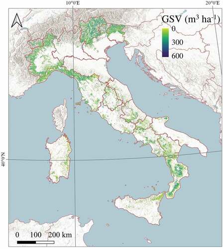
Figure 6. Study area Growing Stock Volume prediction map generated with Approach 1 (w₁ =0.5, w₂ = 0.5).

Conclusion

GSV for Italian forest land covered by ALS was estimated with three approaches using existing ALS, Landsat, and NFI data. Three primary conclusions were drawn from the study. Firstly, CHM and Landsat data are confirmed as a reliable and efficient sources of information for predicting GSV, even in large and complex Mediterranean forest areas. Moreover, the power model facilitates accurate estimation of biological variables such as GSV. Secondly, remotely sensed auxiliary data may contribute to increasing the precision of GSV estimates. Thirdly, ALS data, although fragmentary and acquired in different years, contributes to improved GSV estimates. CHM and Landsat data, increased the efficiency of GSV estimation compared with the standard stratified estimate with the simple expansion estimator within strata for the two approaches, (i) stratified estimation with model-assisted estimation within strata and (ii) stratified estimation with model-assisted estimation within strata and CHM-based pseudo-plots. The total ALS coverage provided the greatest improvement in accuracy with a relative efficiency of 1.33. However, only a portion of forests are covered by ALS currently. Even in a realistic scenario for Italy, with CHM data in only 50% of forests, their contribution increases the accuracy (variance) by a factor of 1.24.

From this perspective, we encourage the Italian NFI to publicly release both NFI plot data, including the exact plot coordinates, for the 3^rd National Forest Inventory for purposes of supporting construction of future RS-based forest maps of GSV or biomass. Lastly, in the future we anticipate that ALS will finally be available wall-to-wall in Italy to facilitate prediction of forest variables with even greater accuracy.

Disclosure statement

No potential conflict of interest was reported by the author(s).

References

- Astola, H., Häme, T., Sirro, L., Molinier, M., & Kilpi, J. (2019). Comparison of sentinel-2 and landsat 8 imagery for forest variable prediction in boreal region. Remote Sensing of Environment, 223, 257–273. https://doi.org/10.1016/j.rse.2019.01.019
- Chirici, G., Giannetti, F., McRoberts, R. E., Travaglini, D., Pecchi, M., Maselli, F., Chiesi, M., & Corona, P. (2020). Wall-to-wall spatial prediction of growing stock volume based on Italian National Forest Inventory plots and remotely sensed data. International Journal of Applied Earth Observation and Geoinformation, 84, 101959. https://doi.org/10.1016/J.JAG.2019.101959
- Chirici, G., McRoberts, R. E., Fattorini, L., Mura, M., & Marchetti, M. (2016). Comparing echo-based and canopy height model-based metrics for enhancing estimation of forest aboveground biomass in a model-assisted framework. Remote Sensing of Environment, 174, 1–9. https://doi.org/10.1016/j.rse.2015.11.010
- Cochran W. G., 1977. Sampling techniques, third edition, New York: John Wiley & Sons, inc.
- Corona, P., Fattorini, L., Franceschi, S., Scrinzi, G., & Torresan, C. (2014). Estimation of standing wood volume in forest compartments by exploiting airborne laser scanning information: Model-based, design-based, and hybrid perspectives. Canadian Journal of Forest Research, 44(11), 1303–1311. https://doi.org/10.1139/cjfr-2014-0203
- D’Amico, G., Vangi, E., Francini, S., Giannetti, F., Nicolaci, A., Travaglini, D., Massai, L., Giambastiani, Y., Terranova, C., & Chirici, G. (2021). Are we ready for a National Forest Information System? State of the art of forest maps and airborne laser scanning data availability in Italy. iForest - Biogeosciences and Forestry, 14(2), 144–154. https://doi.org/10.3832/ifor3648-014
- De Laurentis, D., Papitto, G., Gasparini, P., Di Cosmo, L., & Floris, A., 2021. Italian Forests, Selected results of the third National Forest Inventory INFC 2015. carabinieri command for the protection of biodiversity and parks. Available online: https://www.inventarioforestale.org/sites/default/files/datiinventario/pubb/Sintesi_INFC2015.pdf
- FAO. (2020). Global Forest Resources Assessment 2020: Main report (pp. 184). https://doi.org/10.4060/ca9825en
- Foga, S., Scaramuzza, P. L., Guo, S., Zhu, Z., Dilley, R. D., Beckmann, T., Schmidt, G. L., Dwyer, J. L., Joseph Hughes, M., & Laue, B. (2017). Cloud detection algorithm comparison and validation for operational Landsat data products. Remote Sensing of Environment, 194, 379–390. https://doi.org/10.1016/j.rse.2017.03.026
- FOREST EUROPE, (2015). State of Europe's forest, FOREST EUROPE Liaison Unit Madrid: Ministerial Conference on the Protection of Forests in Europe. https://foresteurope.org/wp-content/uploads/2022/02/soef_21_12_2015.pdf
- Francini S, McRoberts R E, Giannetti F, Marchetti M, Scarascia Mugnozza G, and Chirici G. (2021). The Three Indices Three Dimensions (3I3D) algorithm: a new method for forest disturbance mapping and area estimation based on optical remotely sensed imagery. International Journal of Remote Sensing, 42(12), 4693–4711. 10.1080/01431161.2021.1899334
- Francini S, McRoberts R E, Giannetti F, Mencucci M, Marchetti M, Scarascia Mugnozza G, and Chirici G. (2020). Near-real time forest change detection using PlanetScope imagery. European Journal of Remote Sensing, 53(1), 233–244. 10.1080/22797254.2020.1806734
- Giannetti, F., Chirici, G., Gobakken, T., Næsset, E., Travaglini, D., & Puliti, S. (2018). A new approach with DTM-independent metrics for forest growing stock prediction using UAV photogrammetric data. Remote Sensing of Environment, 213, 195–205. https://doi.org/10.1016/j.rse.2018.05.016. rse.2018.05.016.
- Goodwin N R, Coops N C, and Culvenor D S. (2006). Assessment of forest structure with airborne LiDAR and the effects of platform altitude. Remote Sensing of Environment, 103(2), 140–152. 10.1016/j.rse.2006.03.003
- Gorelick, N., Hancher, M., Dixon, M., Ilyushchenko, S., Thau, D., & Moore, R. (2017). Google Earth Engine: Planetary-scale geospatial analysis for everyone. Remote Sensing of Environment, 202, 18–27. https://doi.org/10.1016/j.rse.2017.06.031
- Gregoire, T. G. (1998). Design-based and model-based inference in survey sampling: Appreciating the difference. Canadian Journal of Forest Research, 28(10), 1429–1447. https://doi.org/10.1139/x98-166
- Gregoire, T. G., Næsset, E., McRoberts, R. E., Ståhl, G., Andersen, H.-E., Gobakken, T., Ene, L., & Nelson, R. (2016). Statistical rigor in Lidar-assisted estimation of aboveground forest biomass. Remote Sensing of Environment, 173, 98–108. https://doi.org/10.1016/j.rse.2015.11.012
- Hijmans, R. J., & van Etten, J., 2012. raster: Geographic analysis and modeling with raster data. R package version 2.0-12. http://CRAN.R-project.org/package=raster
- Holm, S., Nelson, R., & Ståhl, G. (2017). Hybrid three-phase estimators for large-area forest inventory using ground plots, airborne lidar, and space lidar. Remote Sensing of Environment, 197, 85–97. https://doi.org/10.1016/j.rse.2017.04.004
- Hyyppä, J., Hyyppä, H., Leckie, D., Gougeon, F., Yu, X., & Maltamo, M. (2008). Review of methods of small-footprint airborne laser scanning for extracting forest inventory data in boreal forests. International Journal of Remote Sensing. -, 29(5), 1339–1366. https://doi.org/10.1080/01431160701736489
- INFC. (2004).Il disegno di campionamento. Inventario Nazionale delle Foreste e dei Serbatoi Forestali di Carbonio. MiPAF - Direzione Generale per le Risorse Forestali Montane e Idriche, Corpo Forestale dello Stato. ISAFA, Trento, 36. https://www.inventarioforestale.org/sites/default/files/datiinventario/Sch_Cam.pdf
- Jakubowski M K, Guo Q, and Kelly M. (2013). Tradeoffs between lidar pulse density and forest measurement accuracy. Remote Sensing of Environment, 130, 245–253. 10.1016/j.rse.2012.11.024
- Kangas, A., Astrup, R., Breidenbach, J., Fridman, J., Gobakken, T., Korhonen, K. T., Maltamo, M., Nilsson, M., Nord-Larsen, T., Næsset, E., & Olsson, H. (2018). Remote sensing and forest inventories in Nordic countries – Roadmap for the future. Scandinavian Journal of Forest Research, 33(4), 397–412. https://doi.org/10.1080/02827581.2017.1416666
- Kotivuori, E., Korhonen, L., & Packalen, P. (2016). Nationwide airborne laser scanning based models for volume, biomass and dominant height in Finland. Silva Fennica, 50(4), 1567. https://doi.org/10.14214/sf.1567
- Lefsky, M. A, Hudak, A. T, Cohen, W. B, & Acker, S. A. (2005). Geographic variability in lidar predictions of forest stand structure in the Pacific Northwest. Remote Sens. Environ, 95(4), 532–548. https://doi.org/10.1016/j.rse.2005.01.010
- Li, S., Quackenbush, L. J., & Im, J. (2019). Airborne lidar sampling strategies to enhance forest aboveground biomass estimation from Landsat imagery. Remote Sensing, 11(6), 1906. https://doi.org/10.3390/rs11161906
- Lisańczuk, M, Mitelsztedt, K, Parkitna, K, Krok, G, Stereńczak, K, Wysocka-Fijorek, E, & Miścicki, S. (2020). Influence of sampling intensity on performance of two-phase forest inventory using airborne laser scanning. Forest Ecosystems, 7(1), 65. https://doi.org/10.1186/s40663-020-00277-6
- Lu, D., Chen, Q., Wang, G., Liu, L., & Li, G. (2016). A survey of remote sensing-based aboveground biomass estimation methods in forest ecosystems. International Journal of Digital Earth, 9(1) , 1–43. https://doi.org/10.1080/17538947.2014.990526
- Lu D, Chen Q, Wang G, Moran E, Batistella M, Zhang M, Vaglio Laurin G, and Saah D. (2012). Aboveground Forest Biomass Estimation with Landsat and LiDAR Data and Uncertainty Analysis of the Estimates. International Journal of Forestry Research, 2012, 1–16. 10.1155/2012/436537
- Masek, J. G., Vermote, E. F., Saleous, N., Wolfe, R., Hall, F. G., Huemmrich, F., Gao, F., Kutler, J., & Lim, T. K. (2013). LEDAPS calibration, reflectance, atmospheric correction preprocessing code, version 2. model product. ORNL DAAC. https://doi.org/10.3334/ORNLDAAC/1146
- McRoberts, R. E., Chen, Q., Domke, G. M., Ståhl, G., Saarela, S., & Westfall, J. A. (2016b). Hybrid estimators for mean aboveground carbon per unit area. Forest Ecology and Management, 378, 44–56. https://doi.org/10.1016/j.foreco.2016.07.007
- McRoberts, R. E., Chen, Q., Walters, B. F., & Kaisershot, D. J. (2018). The effects of global positioning system receiver accuracy on airborne laser scanning-assisted estimates of aboveground biomass. Remote Sensing of Environment, 207, 42–49. https://doi.org/10.1016/j.rse.2017.09.036
- McRoberts, R. E, Domke, G. M, Chen, Q, Næsset, E, & Gobakken, T, 2016a. Using genetic algorithms to optimize k-Nearest Neighbors configurations for use with airborne laser scanning data. Remote Sensing of Environment. 184, 387–395. 2016.7. 2016. https://doi.org/10.1016/j.rse.2016.07.007
- McRoberts, R. E., Liknes, G. C., & Domke, G. M. (2014). Using a remote sensing-based, percent tree cover map to enhance forest inventory estimation. Forest Ecology and Management, 331, 12–18. https://doi.org/10.1016/j.foreco.2014.07.025
- McRoberts, R. E., Magnussen, S., Tomppo, E. O., & Chirici, G. (2011). Parametric, bootstrap, and jackknife variance estimators for the k-Nearest Neighbors technique with illustrations using forest inventory and satellite image data. Remote Sensing of Environment, 115(12), 3165–3174. https://doi.org/10.1016/j.rse.2011.07.002
- McRoberts, R. E., Naesset, E., & Gobakken, T. (2013). Accuracy and precision for remote sensing applications of nonlinear model-based inference. IEEE Journal of Selected Topics in Applied Earth Observations and Remote Sensing, 6(1), 27–34. https://doi.org/10.1109/JSTARS.2012.2227299
- McRoberts R E, Wendt D G, Nelson M D, and Hansen M H. (2002). Using a land cover classification based on satellite imagery to improve the precision of forest inventory area estimates. Remote Sensing of Environment, 81(1), 36–44. 10.1016/S0034-4257(01)00330-3
- MITE - Italian Ministry of Ecological Transition, 2021. Ministerial decree of 09- 29-2021 online: https://www.mite.gov.it/sites/default/files/archivio/allegati/PNRR/DEC%20398_29_9_2021%20(1).pdf
- Montaghi, A., Corona, P., Dalponte, M., Gianelle, D., Chirici, G., & Olsson, H. (2013). Airborne laser scanning of forest resources: An overview of research in Italy as a commentary case study. International Journal of Applied Earth Observation and Geoinformation, 23, 288–300. https://doi.org/10.1016/j.jag.2012.10.002
- Moser, P., Vibrans, A. C., McRoberts, R. E., Næsset, E., Gobakken, T., Chirici, G., Mura, M., & Marchetti, M. (2017). Methods for variable selection in LiDAR-assisted forest inventories. Forestry, 90(1), 112–124. https://doi.org/10.1093/forestry/cpw041
- Mura, M., Bottalico, F., Giannetti, F., Bertani, R., Giannini, R., Mancini, M., Orlandini, S., Travaglini, D., & Chirici, G. (2018). Exploiting the capabilities of the Sentinel-2 multi spectral instrument for predicting growing stock volume in forest ecosystems. International Journal of Applied Earth Observation and Geoinformation, 66, 126–134. https://doi.org/10.1016/j.jag.2017.11.013
- Næsset, E. (2002). Predicting forest stand characteristics with airborne scanning laser using a practical two-stage procedure and field data. Remote Sensing of Environment, 80(1), 88–99. https://doi.org/10.1016/S0034-4257(01)00290-5
- Næsset, E., Gobakken, T., Holmgren, J., Hyyppä, H., Hyyppä, J., Maltamo, M., M, N., Olsson, H., Persson, Å., & Söderman, U. (2004). Laser scanning of forest resources: The nordic experience. Scandinavian Journal of Forest Research, 19(6), 482–499. https://doi.org/10.1080/02827580410019553
- Nichol, J. E., & Sarker, L. R. (2011). Improved biomass estimation using the texture para- meters of two high-resolution. Optical Sensors, 49(3), 930–948. https://doi.org/10.1109/TGRS.2010.2068574
- Nilsson, M., Nordkvist, K., Jonzén, J., Lindgren, N., Axensten, P., Wallerman, J., Egberth, M., Larsson, S., Nilsson, L., Eriksson, J., & Olsson, H. (2017). A nationwide forest attribute map of Sweden predicted using airborne laser scanning data and field data from the National Forest Inventory. Remote Sensing of Environment, 194, 447–454. https://doi.org/10.1016/j.rse.2016.10.022
- Pagliarella, M. C., Sallustio, L., Capobianco, G., Conte, E., Corona, P., Fattorini, L., & Marchetti, M. (2016). From one-to two-phase sampling to reduce costs of remote sensing-based estimation of land-cover and land-use proportions and their changes. Remote Sensing of Environment, 184, 410–417. https://doi.org/10.1016/j.rse.2016.07.027
- Puliti, S., Saarela, S., Gobakken, T., Ståhl, G., & Næsset, E. (2018). Combining UAV and Sentinel-2 auxiliary data for forest growing stock volume estimation through hierarchical model-based inference. Remote Sensing of Environment, 204, 485–497. https://doi.org/10.1016/j.rse.2017.10.007
- Saarela, S., Holm, S., Grafström, A., Schnell, S., Næsset, E., Gregoire, T. G., Nelson, R. F., & Ståhl, G. (2016). Hierarchical model-based inference for forest inventory utilizing three sources of information. Annals of Forest Science, 73(4), 895–910. https://doi.org/10.1007/s13595-016-0590-1
- Saarela, S., Holm, S., Healey, S. P., Andersen, H. E., Petersson, H., Prentius, W., Patterson, P. L., Næsset, E., Gregoire, T. G., & Ståhl, G. (2018). Generalized hierarchical model-based estimation for aboveground biomass assessment using GEDI and landsat data. Remote Sensing, 10(11) , 1832. https://doi.org/10.3390/rs10111832
- Saarela S, Schnell S, Grafström A, Tuominen S, Nordkvist K, Hyyppä J, Kangas A, and Ståhl G. (2015). Effects of sample size and model form on the accuracy of model-based estimators of growing stock volume. Can. J. For. Res., 45(11), 1524–1534. 10.1139/cjfr-2015-0077
- Särndal, C. E., Swensson, B., & Wretman, J. (1992). Model Assisted Survey Sampling. Springer.
- Tabacchi, G., De Natale, F., Di Cosmo, L., Floris, A., Gagliano, C., Gasparini, P., Genchi, L., Scrinzi, G., & Tosi, V. (2007). Le stime di superficie 2005 - Prima parte. In Inventario Nazionale delle Foreste e dei Serbatoi Forestali di Carbonio, ISAFA. Trento. 413.
- Tabacchi, G., Di Cosmo, L., Gasparini, P., & Morelli, S. (2011). Stima del volume e della fitomassa delle principali specie forestali italiene, Equazioni di previsione, tavole del volume e tavole della fitomassa arborea epigea(pp.415). 978-88-97081-11-1. https://www.inventarioforestale.org/sites/default/files/datiinventario/pubb/tavole_cubatura.pdf
- Tompalski, P., White, J. C., Coops, N. C., & Wulder, M. A. (2019). Demonstrating the transferability of forest inventory attribute models derived using airborne laser scanning data. Remote Sensing of Environment, 227, 110–124. https://doi.org/10.1016/j.rse.2019.04.006
- Waser, L. T., Ginzler, C., & Rehush, N. (2017). Wall-towall tree type mapping from countrywide airborne remote sensing surveys. Remote Sensing, 9(8), 766. https://doi.org/10.3390/rs9080766
- White, J. C., Coops, N. C., Wulder, M. A., Vastaranta, M., Hilker, T., & Tompalski, P. (2016). Remote Sensing Technologies for Enhancing Forest Inventories: A Review. Canadian Journal of Remote Sensing, 42(5), 619–641. https://doi.org/10.1080/07038992.2016.1207484
- White, J. C., Wulder, M. A., Hobart, G. W., Luther, J. E., Hermosilla, T., Griffiths, P., Coops, N. C., Hall, R. J., Hostert, P, Dyk, A, & Guindon, L. (2014). Pixel-based image compositing for large-area dense time series applications and science. Canadian Journal of Remote Sensing, 40(3), 192–21. https://doi.org/10.1080/07038992.2014.945827
- Wulder M A, Bater C W, Coops N C, Hilker T, and White J C. (2008). The role of LiDAR in sustainable forest management. The Forestry Chronicle, 84(6), 807–826. 10.5558/tfc84807-6
- Wulder, M. A., Loveland, T. R., Roy, D. P., Crawford, C. J., Masek, J. G., Woodcock, C. E., Allen, R. G., Anderson, M. C., Belward, A. S., Cohen, W. B., Dwyer, J., Erb, A., Gao, F., Griffiths, P., Helder, D., Hermosilla, T., Hipple, J. D., Hostert, P., Hughes, M. J, Zhu, Z. (2019). Current status of Landsat program, science, and applications. Remote Sensing of Environment, 225, 127–147. https://doi.org/10.1016/j.rse.2019.02.015
- Yun, T., Jiang, K., Li, G., Eichhorn, M. P., Fan, J., Liu, F., Cao, L., An, F., & Cao, L. (2021). Individual tree crown segmentation from airborne LiDAR data using a novel Gaussian filter and energy function minimization-based approach. Remote Sensing of Environment, 256, 112307. https://doi.org/10.1016/j.rse.2021.112307
- Zhao, P., Lu, D., Wang, G., Wu, C., Huang, Y., & Yu, S. (2016). Examining spectral reflectance sa- turation in landsat imagery and corresponding solutions to improve forest above- ground biomass estimation. Remote Sensing, 8(6), 469. https://doi.org/10.3390/rs8060469