Satellite thermographies as an essential tool for the identification of cold air pools: an example from SE Spain

ABSTRACT

The processes involved in the formation of nocturnal temperature inversions (NTIs) are of great relevance throughout the year, notably influencing the surface distribution of minimum temperatures during nights of atmospheric stability. The low density of surface meteorological stations in the study area motivated the use of thermographies for the mapping and identification of cold air pools CAPs. Thermal distribution during stable nights leads to the formation of CAPs in valley areas and depressed areas, and in areas with warmer air (WAM) in orographically complex areas. The thermographies carried out with satellite products from AQUA and SUOMI-NPP (MODIS and VIIRS LST) represent the only tool capable of fully radiographing the territory under study, thus overcoming the limitations in the interpolation of minimum surface temperatures. The main objective of the research was, therefore, to value thermography as an important tool in the identification of CAPs. The products used were subjected to statistical validation with the surface temperatures recorded in meteorological observatories (R² 0.87/0.88 and Bias −1.2/-1.3) with a new objective of making thermal distribution maps in nocturnal stability processes …

KEYWORDS:

• Inversion
• cold
• thermographies
• validation
• tool

Introduction

The need for spatial information and real-time access to new meteorological data has led to a growing scientific interest in seeking new satellite methodologies to fill in existing climate gaps. The ability to obtain spatial temperature estimates at high temporal (daily) and spatial (1 km) resolution appeared in 1981 with the launch of the Advanced Very High Resolution Radiometer (AVHRR) aboard the National Oceanic and Atmospheric Administration (NOAA) satellite, and later, in 1999, with the Moderate Resolution Imaging Spectroradiometer (MODIS) aboard the Aqua and Terra satellites.

There is an important relationship between land surface temperature (LST) and near surface air temperature (T air), in orographically complex terrain, with a lower density of observational data, these differences are amplified (Mutiibwa et al., 2015).

Recent advances in remote sensing instruments and computing power, together with improvements in parameterizations and numerical algorithms, permit detailed analyses of possible cold air accumulations in valley bottoms. Zhong et al. (2001) summarized the characteristics of CAPs that appeared during 4 months of observation, with the application of satellite images and surface temperature data collected over a period of 10 years in the lower Columbia basin. The focus of this study was to evaluate the relative importance of different physical mechanisms in the formation and maintenance of persistent cold air pockets in winter, and the applicability of satellite images for their study. Different recent studies have examined the life cycles of CAPs (Flores et al., 2020; Foster et al., 2017; Katurji & Zhong, 2012; Lareau, 2014; Zängl, 2005).

Crops located in topographically depressed places are more vulnerable to irradiation frosts, which are very common during stable nights in SE Spain. During the last few decades, interpolation methods have been used to estimate minimum temperatures in low-altitude areas, but they have always been subject to important limitations due to the low density of meteorological observatories, especially in areas of higher altitude and lower population density. Jarvis and Stuart (2001) used a geographic information system (GIS) to find local watersheds and cold pools in the UK. They did not find a statistical significance for a spatial resolution of 1 km. Spatial interpolation, therefore, has been widely applied for the mapping of minimum temperatures in mountainous areas (Bolstad et al., 1998; Thornton et al., 1997). Most spatial interpolation models for minimum temperature estimation incorporate a vertical gradient correction to accommodate the difference in elevation (Dodson & Marks, 1997; Nalder & Wein, 1998). The gradient varies temporally on seasonal, daily, and even hourly scales. Therefore, although the interpolation method has been widely applied to estimate minimum temperatures during NTI phenomena, its spatial and vertical limitations restrict its use, despite the latest applied methodologies, using non-linear profiles and non-Euclidean distances (Frei, 2014).

In addition, the spatial distribution of near-surface air temperature over a coastal mountain range in southern Chile (Nahuelbuta Mountains) is investigated by in situ measurements, satellite-derived LST, and simulations during the austral winter from 2011 (González & Garreaud, 2019).

In recent years, important advances in remote sensing have led to the development of new algorithms and equations that provide the air temperature at 1.5 m height (Ta) using the LST, obtained from remote satellite sensor images (Vancutsem et al., 2010; Zhu et al., 2013).

The LST products of different sensors (MODIS, SUOMI NPP, NOAA20, AVHRR …) have been used successfully in various scientific fields; for example, for estimation of evapotranspiration (Anderson et al., 2011) and the temperature of the air (Vancutsem et al., 2010) and for urban heat island monitoring (Rajasekar & Weng, 2009), or trends and transitions in the growing season Normalized Difference Vegetation Index (NDVI) for changes of large wildfires (Potter & Alexander, 2019). The use of LST products can aid the development of long-term moderate resolution LST climate data records (Yu et al., 2008).

The great spatial and temporal (daily) resolution provided, open data, and easy access to satellite images have generated a significant increase in studies using Ta (Noi et al., 2016; Sismanidis et al., 2016; Zhou et al., 2017), especially using information from the Visible Infrared Imaging Radiometer Suite (VIIRS) instrument on board the Suomi National Polar-Orbiting Partnership (Suomi NPP) satellite (Hillger, 2013). The products generated by the Moderate Resolution Imaging Spectroradiometer (MODIS6) sensor, which travels aboard the Terra in 1999 and Aqua in 2002 satellite platforms (Wan et al., 2015), are also widely used.

Terrestrial air surface temperature (Ta), also called “air temperature” or “ near surface air temperature “, data are generally collected as point data from weather station locations, typically within 2 m of the Earth’s surface. In general, Ta values obtained from weather stations have very high temporal resolution and precision, but do not capture information for an entire region and therefore may not be suitable for spatial modeling applications. The Moderate Resolution Imaging Spectroradiometer (MODIS) sensor on board the Terra and Aqua platforms produces high-quality LST products from data that have a number of strengths (Wan & Li, 2010). They include global coverage, high radiometric resolution and wide dynamic ranges, exact geolocation (Wolfe, 2006), and high thermal infrared (TIR) calibration precision used in LST recovery (Barnes et al., 1998).

In recent years, different studies have used the Earth’s surface temperature (LST) obtained from remote sensor images to estimate Ta, due to the high spatial and temporal resolution, free availability, and easy access to the satellite images. The difference between LST and Ta is strongly influenced by surface characteristics and atmospheric conditions.

Based on analytical results, the TVX method was applied for the first time using air temperature observations made in 2009 for model calibration (Zhu et al., 2013). Subsequently, the calibrated TVX method was run in a sliding window mode to produce complete image coverage for the study area.

The Earth’s LST is one of the parameters that are indispensable for the estimation of air temperature by various satellite-based methods (Zhu et al., 2013). According to Vancutsem et al. (2010), two approaches to the estimation of Ta from LST can be distinguished: one is for minimum temperatures (Ta), another is for maximum temperatures (Ta). During the night, as solar radiation does not affect the thermal infrared signal, the recovery of Ta (minimum) is simpler, and there is a good relationship between LSTs and Ta (Jones et al., 2004; Mostovoy et al., 2006).

The application of records of the LST, measured by satellite sensors such as MODIS, to recover the number of frost days was proposed by Hachem et al. (2009) for the modeling analysis of permafrost in non-mountainous terrain (Langer et al., 2013; Westermann et al., 2012), and provided a good statistical correlation between LST and Ta for most of the stations analyzed. Aqua MODIS products are considered to be accurate enough to spatially represent the Ta (minimum) at a 1-km resolution, allowing this temperature to be monitored operationally.

The nighttime LST data from Terra (LSTmodn) proved to be accurate enough for the linear estimation of mean temperatures (Tmean) and mean minimum temperatures (Tmin) with a strong correlation (R² > 0.90) and minimal bias (RMSE and MD <7 K). However, in the mountainous areas of southwest China, in a complex topography, the thermal mechanism is more complicated. The results obtained there suggest that a large terrain relief can significantly influence the spatial pattern of the climate and, therefore, modify the flow of energy from the surface (Lin et al., 2016).

The main objective of the present work was to produce a high resolution mapping of winter night air temperatures during stable early mornings (subject to NTI processes). Thermography is a tool with a great capacity to spatially encompass the entirety of a territory, thus making up for the shortcomings and limitations of temperature interpolation based on the data from meteorological observatories. The study area shows a low density of meteorological stations, especially in the western and mountainous areas of the basin. The validation of the satellite products used (MODIS and VIIRS LST) was the second major objective, fundamental for the cartography generated to be as reliable as possible. The nocturnal satellite images were analyzed from the space-time point of view in southeastern Spain, using a statistical comparison of the analyzed products with the surface temperatures recorded at meteorological observatories. The thermographs generated reflect the spatial distribution of night temperatures in the study area. The third major objective was to identify the main CAPs in southeastern Spain, together with their extension, delimitation, and intensity. High resolution mapping was performed on a county scale. For the minimum temperatures, of extraordinary complexity in the territory, the use of new tools was required to identify the coldest sites, key for many sectors, but especially in agricultural planning.

Study area

The study area is the Segura River Basin, one of the most important in Spain (Figure 1). It is located in the southeast of Spain, with an approximate area of 19,025 km², covering almost the entire province of Murcia (11,180 km²), a large sector in the south of the province of Albacete (4759 km²), and relatively small sectors from the provinces of Granada, Jaén, and north of Almería (1787 km²), and finally the south of Alicante (1,299 km²).

Figure 1. a) Study area and the meteorological stations used to verify the hourly surface temperatures, b) an example of the original file of the VIIRS LST product from December 4, 2017.

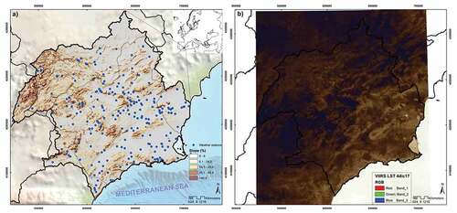
Orographically, it is a territory with a great altitude contrast, notable slopes, and a great variety of landscapes, mainly due to a very heterogeneous climate. It is located at a 38°N latitude, an area of transition between cool-humid climates (disturbances of the polar front) and temperate-dry (subtropical anticyclones). The climate obtains eminently Mediterranean features, due to its location on a western facade of the continent.

A multitude of climatic types appear (1981–2010) according to the Köppen-Geiger classification. Csb (oceanic Mediterranean climate, or oceanic transition) in western mountainous areas, typical Mediterranean climate (Csa), steppe or semi-arid climate (BSk), warm semi-arid (BSh) and hot desert or Saharan climate (BWh) in coastal areas.

Materials

The cartography of the surface night temperatures was generated using products from the AQUA and SUOMI-NPP satellites (MODIS LST and VIIRS LST), obtained from the websites https://earthexplorer.usgs.gov/ and https://worldview.earthdata.nasa.gov/.

MODIS LST (MYD11A1 V6)

The MODIS LST product is extracted from the MODIS6 sensor (Moderate Resolutions Imaging Spectroradiometer), which travels aboard the Terra in 1999 and Aqua in 2002 satellite platforms. This sensor has a scanning width of 2300 km, providing a complete view of the Earth every 1 or 2 days. It acquires data in 36 spectral channels with high radiometric sensitivity (12 bits). Its spectral channels range from 0.4 to 14.4 μm, covering the spectral regions of the visible (VIS), near infrared (NIR), short wave infrared (SWIR), medium wave infrared (MWIR), and long wave infrared (LWIR). The products are produced by NASA (National Aeronautics and Space Administration) through its EOS (Earth Observation System) program and are distributed by LP DAAC (The Land Processes Distributed Active Archive Center; Opazo & Chuvieco, 2007). The MYD11A1 V6 (MODIS LST) product provides daily LST and emissivity values on a 1200 × 1200 kilometer grid. The temperature value is derived from the sweep product MOD11_L2. Each MYD11A1 data file includes the nighttime LST image (for Terra at ~ 22:30 UTC and for Aqua at ~ 01:30 UTC). For the analysis described in this paper, the Aqua image was used, due to its greater hourly proximity to the minimum temperature recorded during the early morning.

VIIRS LST (Band I5)

For its part, the VIIRS LST product is obtained from the VIIRS instrument on board the SUOMI-NPP satellite. It is a scanning radiometer that measures radiances on a global scale in the visible and infrared spectra over the land, atmosphere, cryosphere, and oceans (Hillger, 2013). Among the 22 bands there are five high resolution image channels (I bands), 16 moderate resolution channels (M bands), and one day/night band (DNB; Cao et al., 2013). The by-product Band I5 is used specifically (it´s a gloss temperature layer calculated from calibrated radiances of VIIRS (VNP02), with a spatial resolution of 375 m and a daily temporal resolution. The measurement bias and precision specified for the product are 1.4 and 0.5 K, respectively, which must be met when the cloud mask indicates high confidence under clear conditions (Minnett et al., 2014). It has a synchronous solar orbit at an altitude of 829 km, and passage times over the vertical of the study area between 1.40 and 2.40 in the morning (Niclòs et al., 2018).

The VIIRS is one of the key instruments of the SUOMI NPP satellite. The successful launch of the SUOMI NPP satellite, with VIIRS on board, on 28 October 2011, gave rise to a new generation of capabilities in operational environmental remote sensing for climatic, oceanic, and other environmental applications (Cao et al., 2013; Hutchinson & Cracknell, 2006; Lee, 2006). It has a resolution of 0.7 * 0.8 km and a total of 3,200 * 3,200 columns (Minnett et al., 2014). The product is generated at all ground pixels, except when the conditions mentioned above are not met, as determined from the VIIRS Cloud Mask (VCM; Justice et al., 2013).

In this work, for the validation of the VIIRS/MODIS LST products, the air surface temperatures recorded at 219 meteorological observatories with hourly data were used. These observatories belong to the Sistema Automático de Información Hidrológica (SAIH) of the Confederación Hidrográfica del Segura (CHS) and the Sistema de Información Agrario de Murcia (SIAM) network of the Instituto Murciano de Investigación y Desarrollo Agrario y Alimentario (Figure 1).

Methods

MODIS LST (MYD11A1 V6)

Above 30° latitude, some pixels may have multiple observations where clear sky criteria are met. When this occurs, the pixel value is the average of all the rated observations, with new methodologies recently developed (termed the “pixel-to-pixel correction (PPC) method”; Xu et al., 2016). It is also provided together with the day and night surface temperature bands and their MODIS quality indicator, bands 31 and 32, and six observation layers (Wan et al., 2015; Equation 1)(1) $\begin{array}{rl}& \mathrm{L}\mathrm{S}\mathrm{T}={\mathrm{b}}_0+(({\mathrm{b}}_1+({\mathrm{b}}_2(1-\epsilon /\epsilon ))\\ & +({\mathrm{b}}_3((\mathrm{\Delta }\epsilon /{\epsilon }^2))){\mathrm{T}}_{31}+{\mathrm{T}}_{32}/2\\ & +((({\mathrm{b}}_4+({\mathrm{b}}_5(1-\epsilon /\epsilon ))\\ & +({\mathrm{b}}_6(\mathrm{\Delta }\epsilon /{\epsilon }^2))){\mathrm{T}}_{31}-{\mathrm{T}}_{32}/2\end{array}$(1) .

(1) $\begin{array}{rl}& \mathrm{L}\mathrm{S}\mathrm{T}={\mathrm{b}}_0+(({\mathrm{b}}_1+({\mathrm{b}}_2(1-\epsilon /\epsilon ))\\ & +({\mathrm{b}}_3((\mathrm{\Delta }\epsilon /{\epsilon }^2))){\mathrm{T}}_{31}+{\mathrm{T}}_{32}/2\\ & +((({\mathrm{b}}_4+({\mathrm{b}}_5(1-\epsilon /\epsilon ))\\ & +({\mathrm{b}}_6(\mathrm{\Delta }\epsilon /{\epsilon }^2))){\mathrm{T}}_{31}-{\mathrm{T}}_{32}/2\end{array}$(1)

where ε and Δε are the mean of and the difference between the emissivities in bands 31 and 32. The coefficients of the algorithm bk (with k = 0–6) depend on the display of the zenith angle, the air temperature at the surface (T air), and the atmospheric water vapor content.

In the LST recovery algorithm for the MYD11A1 product, the emissivity method is based on the classification used to estimate the emissivity in the MODIS 31 band (10.78 to 11.28 μm) and the MODIS 32 band (11.77 to 12.27 μm), and the generalized split-window algorithm is used to generate the LST product 12.26 (Wang et al., 2019).

VIIRS LST (Band I5)

The VIIRS LST product (Band I5) uses the split window algorithm (Yu et al., 2008) through to the brightness temperature (Ti) measured in two VIIRS spectral bands: M15, placed at 10.76 mm (i = 15), and M16, set at 12.01 mm (i = 16). Different sets of coefficients (aj, with j = 0–4) are used for day and night and for 17 surface types from the classification maps of the International Geosphere-Biosphere Program (IGBP; Guillevic et al., 2014; Liu et al., 2015).

The baseline is a split window (SW) algorithm that applies measured brightness temperatures in the VIIRS M15 and M16 bands, centered at wavelengths of 10.8 µm and 12.0 µm, respectively (Sun & Pinker, 2003; Schroeder & Giglio, 2017). The optional double division window (DSW) algorithm applies two additional infrared shortwave bands: M12 and M13, centered at wavelengths of 3.75 μm and 4.0 μm, respectively. The product has operated using a single split window algorithm, which is insensitive to solar radiation (Yu et al., 2008). The Nighttime DSW Algorithm is used (Equation 2(2) $\mathrm{L}\mathrm{S}\mathrm{T}\mathrm{i}=\mathrm{b}0\left(\mathrm{i}\right)+\mathrm{b}1\left(\mathrm{i}\right)\mathrm{T}11++\mathrm{b}2\left(\mathrm{T}11-\mathrm{T}12\right)+\mathrm{b}1.\text{break}\left(\mathrm{i}\right)\hspace{0.17em}\left(\mathrm{s}\mathrm{e}\mathrm{c}\theta -1\right)+\mathrm{b}4\left(\mathrm{i}\right)\mathrm{T}3.75+\mathrm{b}5\left(\mathrm{i}\right)\mathrm{T}4.0+\mathrm{b}6\text{break}\left(\mathrm{i}\right)\mathrm{T}3.752+\mathrm{b}7\left(\mathrm{i}\right)\mathrm{T}4.02+\mathrm{b}8\left(\mathrm{i}\right)\hspace{0.17em}\text{break}{\left(\mathrm{T}11-\mathrm{T}12\right)}^2$(2) ):

(2) $\mathrm{L}\mathrm{S}\mathrm{T}\mathrm{i}=\mathrm{b}0\left(\mathrm{i}\right)+\mathrm{b}1\left(\mathrm{i}\right)\mathrm{T}11++\mathrm{b}2\left(\mathrm{T}11-\mathrm{T}12\right)+\mathrm{b}1.\text{break}\left(\mathrm{i}\right)\hspace{0.17em}\left(\mathrm{s}\mathrm{e}\mathrm{c}\theta -1\right)+\mathrm{b}4\left(\mathrm{i}\right)\mathrm{T}3.75+\mathrm{b}5\left(\mathrm{i}\right)\mathrm{T}4.0+\mathrm{b}6\text{break}\left(\mathrm{i}\right)\mathrm{T}3.752+\mathrm{b}7\left(\mathrm{i}\right)\mathrm{T}4.02+\mathrm{b}8\left(\mathrm{i}\right)\hspace{0.17em}\text{break}{\left(\mathrm{T}11-\mathrm{T}12\right)}^2$(2)

where i is the index of 17 types of IGBP surfaces; aj (i), bj (i), and cj (i) are the regression coefficients of the algorithm in which j represents the sequential position of the term in the equation; T3.75, T4.0, T11, and T12 are the brightness temperatures of the VIIRS bands M12, M13, M15, and M16, respectively; θ is the zenith angle of the satellite and φ is the solar zenith angle. The DSW algorithm consists of day and night versions, and was applied as a reference algorithm before 10 August 2012.

Statistical verification of products

The elaboration of the final cartography shown in this chapter (thermographs with LST), using the MODIS LST and VIIRS LST products, was carried out with the average of 100 maps for each of the products. These refer to 100 stable early mornings (with NTI processes), free of cloud cover (0%) and chosen based on the analysis of minimum surface temperature data and data from atmospheric soundings during the last observation winters: 2017–2018, 2018–2019, and 2019–2020 (Fig. 1). General mapping performed with MODIS/VIIRS LST products provided thermal difference, standard deviation, and statistical correlation results. Likewise, a thermal profile was generated from the final product of the combination between MODIS and VIIRS LST, which allowed a better visualization of the thermal contrasts between CAPs and orographically complex spaces with warm advection (WAM).

For the statistical analysis at the spatial level, net points were generated for the comparison of the different satellite products used (VIIRS LST and MODIS LST) with the surface temperatures recorded at meteorological observatories. First, a homogeneous distribution mesh was created in the study area, having a total of 1293 points (Figure 2a), with a density of one point per 13.9 km². Meanwhile, the analysis of the CAP and WAM areas was carried out using a layer of 1150 points for the CAP areas and one of 3055 points for the WAM areas (Figure 2b).

Figure 2. Net points created for the statistical analysis in: a) the complete study area, and b) CAPs (thermal inversion zones, with blue circles) and WAM (warm air in orographically complex terrain, in green circles).

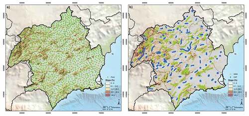
With the “Extract Multi Values to point” function of the ArcGis 10.3 software, plate text files (txt) were exported with information on values corresponding to the average of the MODIS LST and VIIRS LST products, altimetric values (m), orographic difference (%), and temperatures from 219 meteorological observatories for all points generated. For the analysis of the statistical correlations between the VIIRS/MODIS LST products and the surface air temperatures recorded at the meteorological stations (ST), correlations were performed for altitudinal bands (> 1200 m, from 1200 to 600 m, and less than 600 m), for altitudinal difference (> 35%, from 15 to 34%, and less than 15%), or by geographical area in CAP or WAM areas. For this, different statistical tests were used according to the type of statistical distribution.

The Shapiro Wilk statistical test is used to contrast the normality (normal distribution or not) of a data set (Shapiro et al., 1998). It is used to verify whether a data set follows a normal distribution or not. This is of vital importance because the subsequent statistical analyses require the normality of the data. If the sample is normal, Pearson’s linear correlation test (Equation 3(3) $\mathrm{W}=1/{\mathrm{n}}^2({{\mathrm{\Sigma }}^{\mathrm{h}}}_{\mathrm{j}=1}{\mathrm{a}}_{\mathrm{i}\mathrm{n}}{\left({\mathrm{x}}_{\mathrm{n}}-\mathrm{i}+1-{\mathrm{x}}_{\mathrm{i}}\right)}^2$(3) ) is applied:

(3) $\mathrm{W}=1/{\mathrm{n}}^2({{\mathrm{\Sigma }}^{\mathrm{h}}}_{\mathrm{j}=1}{\mathrm{a}}_{\mathrm{i}\mathrm{n}}{\left({\mathrm{x}}_{\mathrm{n}}-\mathrm{i}+1-{\mathrm{x}}_{\mathrm{i}}\right)}^2$(3)

where: n² is the sample variance and the coefficients a_in are usually tabulated in manuals.

In contrast, if either of the two variables of the analyzed sample presents asymmetry and, therefore, does not follow a normal distribution according to the Shapiro-Wilk test, the non-parametric test of the Spearman correlation coefficient is applied. This test examines the strength and direction of the monotonic relationship between two continuous or ordinal variables. The value of the correlation coefficient can vary from −1 to +1. The higher the absolute value of the coefficient, the stronger the relationship between the variables.

The Spearman correlation coefficient, ρ (rho), is a measure of the correlation (the association or interdependence) between two random variables (both continuous and discrete). To calculate ρ, the data are ordered and replaced by their respective order (Equation 4(4) $\mathrm{r}\mathrm{R}=\frac{1-\left(6\mathrm{\Sigma }\mathrm{i}\mathrm{d}\mathrm{i}2\right)}{\mathrm{n}\left(\mathrm{n}2-1\right)}$(4) ):

(4) $\mathrm{r}\mathrm{R}=\frac{1-\left(6\mathrm{\Sigma }\mathrm{i}\mathrm{d}\mathrm{i}2\right)}{\mathrm{n}\left(\mathrm{n}2-1\right)}$(4)

where n = the number of data points of the two variables and di = the rank difference of element “n”

In this study, we also applied two defined cost functions – the bias and the root mean square error (RMSE) – to the relationship between the LST simulated in the MYD11A1 V6 and Band I5 and the observed surface temperature. The mean square error or root mean square deviation (RMSE) measures the amount of error existing between two data sets, that is, a predicted value and an observed or known value (Equation 5(5) $\text{RMSE}=\frac{\sqrt{\sum i=1^n\left(P_i+O_i\right)}}{\text{n}}2$(5) ; Chai & Draxler, 2014). The RMSE, therefore, is ideal for the validation of the temperature estimates of the Band I5 product (predicted) and the temperatures recorded in meteorological stations (observed or known). This statistic has been used in the validations of numerous products – such as MODIS, Band I5 … (Duan et al., 2019; Guillevic et al., 2014; Li et al., 2014).

(5) $\text{RMSE}=\frac{\sqrt{\sum i=1^n\left(P_i+O_i\right)}}{\text{n}}2$(5)

where: Σ is the summation, Pi is the predicted value for the observation in the data set, O_i is the observed value for the observation in the data set, and n is the sample size

The bias is a measure of the “accuracy” of the measurement system and represents the systematic error of the system. It is the contribution to the total error due to the combined effects of all sources of variation, known or unknown (Voinov & Nikulin, 1993). This statistical study is performed through a t test student hypothesis of a sample and a constant, with the following hypotheses. When the p value is greater than 0.05, the null hypothesis is accepted and we can conclude that the measurement system does not present any bias (Equation 6(6) $\text{Bias}\left({}^{^}\theta {}_S,\theta \right)=E_s{\text{D}}^m\left[{}^{\text{^}}\theta {}_{\text{S}}\right]-\theta$(6) ).

(6) $\text{Bias}\left({}^{^}\theta {}_S,\theta \right)=E_s{\text{D}}^m\left[{}^{\text{^}}\theta {}_{\text{S}}\right]-\theta$(6)

where E_s denotes the expected value over the statistical distribution and ^ θ serves as an estimator of θ based on any observed data.

Results

Statistical validation of VIIRS and MODIS LST products with surface temperatures from meteorological observatories (ST)

The thermographs or thermal “radiographs” produced using satellite bands show a significant correlation with the observed surface temperatures. After calculating the statistical average, a statistical correlation was obtained (with an R² of 0.87) with the LST products (Figure 3a and 3b). In addition, the two products have a very high statistical correlation with each other (0.91). All the resulting correlations show highly robust statistical significance, with a confidence level of 0.99 according to the Pearson and Spearman statistical correlations. The thermal difference of the products from the values of the 219 meteorological stations analyzed is 1.7 K. Therefore, the thermographs indicate surface temperatures (ST) somewhat colder than the air temperature (Ta) 1.5 m above the ground (meteorological stations).

Figure 3. The bias, RMSE, and statistical correlation for the relationship between the analyzed MODIS/VIIRS LST products and the surface temperatures recorded at meteorological stations (TS), in the whole study area: a) MODIS LST and b) VIIRS LST; and for the CAP zones: c) MODIS LST and d) VIIRS LST. Solid g reen line show linear regression, dashed red line is nonparametric estimate of the mean, dashed blue line is nonparametric estimate of the variance, and blue shaded area is data-concentration ellipse.

The spatial statistical correlations are relevant for MODIS LST (R² of 0.83), and VIIRS LST (R² of 0.84), undoubtedly solid results with confidence levels of 0.99 and more than 1200 statistical correlation points. The global data of MODIS and VIIRS LST in the study area as a whole show RMSE and bias values of 2.6/2.7 K and −1.2/-1.3 K, respectively, which indicates good statistical fits (Figure 3a and 3b). For both products, the highest statistical correlations are for low-altitude areas, less than 600 m, with an R² of 0.84, and surfaces with little slope (<14%) (Table 4.4). However, for meteorological stations at intermediate altitude (600–1200 m), and in steep areas (> 35% slope), the results are not so good, although they are statistically significant (R² from 0.63 to 0.48). The global results for the CAP zones indicate statistical correlations of −0.75 and −0.76, with a bias and RMSE between 1.5 and 3.8 K (Figure 3c and 3d).

The combination of the MODIS LST and VIIRS LST products shows a spatial statistical correlation with an R² of 0.83 (with more than 3000 correlation points) and a p-value <0.00001. Therefore, this corroborates the excellent statistical fit achieved in the elaboration of high resolution thermographies.

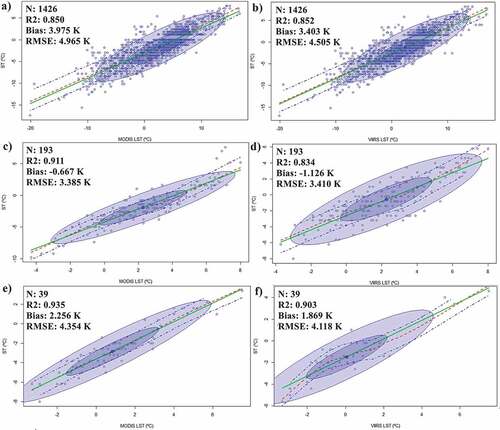
The thermal differences between the analyzed products and the temperatures recorded at the meteorological stations are relatively important (bias between 0 and 4 K). The best fits were obtained for territories located above 1200 m altitude and for orographic slopes between 15 and 34% (bias around 0 K) (Figure 4e and 4f). However, despite giving the best spatial statistical correlations, the low altitude areas (<600 m) gave the highest biases (from 4 to 5 K). Similarly, the differences are more important in flat areas with little slope (<14%), with values of 3.0 to 4.0 K (Figure 5a y 5b). This is due to the influence exerted by the surface temperatures near the coast, with a notable influence of the sea breeze.

Figure 4. The bias, RMSE, and statistical correlation calculated for the relationship between the analyzed MODIS/VIIRS LST products and the surface temperatures recorded at meteorological stations (TS) in the study area, for altitudes 0-600 m: a) MODIS LST and b) VIIRS LST; 601 to 1200 m: c) MODIS and d) VIIRS; and > 1200 m: e) MODIS and f) VIIRS. Solid green line show linear regression, dashed red line is nonparametric estimate of the mean, dashed blue line is nonparametric estimate of the variance, and blue shaded area is data-concentration ellipse.

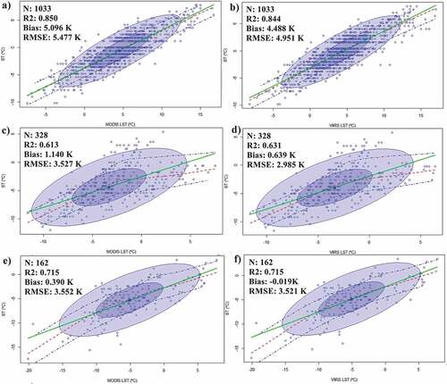
Figure 5. The bias, RMSE, and statistical correlation calculated for the relationship between the analyzed MODIS/VIIRS LST products and the surface temperatures recorded at meteorological stations (TS) in the study area, for orography slopes of 0-14%: a) MODIS LST and b) VIIRS LST; 15-34%: c) MODIS and d) VIIRS; and > 35%: e) MODIS and f) VIIRS. Solid green line show linear regression, dashed red line is nonparametric estimate of the mean, dashed blue line is nonparametric estimate of the variance, and blue shaded area is data-concentration ellipse.

The spatial correlation is somewhat more important within the CAPs than in the zones outside the thermal inversion (WAM), R² being 0.76 and 0.75, respectively (Figure 3c and 3d). In addition, the CAP areas are those with the least bias (1.6 and 2.1 K for VIIRS and MODIS LST, respectively; Table 1), whereas in the WAM areas the bias exceeds 4 K for both products. This is important, since, with high spatial statistical correlation and relatively low thermal differences within the CAPs, it is possible to identify the large pools of cold air in a territory.

Table 1. Statistical summary (R², Bias, and RMSE) of the relationship between the VIIRS/MODIS LST products and the surface temperature (ST). According to the result of the Shapiro-Wilk test (the normality of the sample), the “S” (Spearman) or “P” (Pearson) test is used.

		MODIS LST				VIIRS LST
	Test	Shapiro Wilk	R^2	Bias	RMSE	Shapiro Wilk	R^2	Bias	RMSE
ST	S/S	7.512e-09	0.872	−1.205	2.636	1.95e-07	0.878	−1.334	2.712
ST >1200 m	S/S	4.892e-05	0.715	0.390	3.552	0.00020	0.715	−0.019	3.521
ST1200-601 m	P/P	0.01878	0.613	1.140	3.257	0.05193	0.631	0.639	2.985
ST 600–0 m	S/S	0.00014	0.850	5.096	5.477	0.00092	0.844	4.488	4.951
ST >35%	P/P	0.0559	0.935	2.256	4.354	0.0681	0.903	1.869	4.118
ST 34–15%	S/S	0.0006	0.911	−0.667	3.385	0.0011	0.834	−1.126	3.410
ST 14–0%	S/S	1.42e-11	0.850	3.975	4.965	2.68e-09	0.852	3.403	4.505
ST CAP	S/P	0.00839	0.754	2.141	3.865	0.0169	0.758	1.572	3.494
ST WAM	P/P	0.09123	0.688	4.684	4.921	0.3098	0.715	4.334	4.574

In general, the statistical results provided by the MODIS and VIIRS LST products are very similar. Therefore, they are two data sources of excellent quality for the representation of the distribution of nighttime surface temperatures and the identification of CAPs. On this basis, the two products were subjected to a comparative analysis.

The cartography generated the greatest bias between the MODIS/VIIRS LST products and the ST, at a spatial level, in the northeastern-most sector of the study area: specifically, in the Abanilla-Fortuna Basin, the northern Vega Baja (Pinoso area), and the easternmost sector of the Altiplano of the Murcia Region. VIIRS LST provided better fits than MODIS LST, which gave higher thermal differences in the aforementioned sectors, especially between the Abanilla-Fortuna Basin and the interior of the province of Alicante (Figure 6a and 6b).

Figure 6. Bias (K) between ST and a) MODIS LST and b) VIIRS LST; statistical correlation (Spearman’s R2) between ST and c) MODIS LST and d) VIIRS LST; e) average thermal difference between the VIIRS and MODIS LST products (cream to red colors show that higher temperatures are reported by the MODIS sensor, and, vice versa, blue or cold colors indicate that the MODIS sensor reports lower temperatures); f) standard deviation (K) of the 50 days analyzed for VIIRS and MODIS LST.

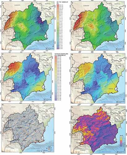
However, the best spatial statistical fits are for elevated areas: specifically, in the central sectors of the northwest part of Murcia Region and in the headwaters of the Segura River (Segura and Alcaraz mountain ranges). Different zones also show thermal differences that are not particularly high (1–2 K). These are the following geographical areas: the south of the province of Albacete (Elche de la Sierra – Socovos), the coastline of Mazarrón-Cartagena, the Highlands of Lorca, the more rugged sectors of the Vega Alta and Media del Segura, the north of the province of Almería (Almanzora), and, in general, the entire northwest part of Murcia Region (Figure 6c and 6d).

The best statistical correlations of the products with the LST appear in the Highlands of Lorca, the Almería plateau (María-Chirivel), the Abanilla-Fortuna Basin, and the north of the study area (Pétrola-Chinchilla). These geographical areas exhibit an R² greater than 0.80.

Somewhat more modest but equally robust (99% confidence level) correlations, between 0.50 and 0.60, exist in the Segura and Alcaraz mountains (the head of the study area), in littoral areas of the province of Alicante, and in the Cartagena field. That is, the eastern and western extremes of the study area (Figure 6e). The bias of the two products is similar (0.4 K), with a very high statistical correlation (R² 0.91). As shown in Figure 6e, most of the study area registers a minimum bias, with practically similar temperatures. In the areas shown in blue tones, the MODIS product reports a slightly lower temperature than the VIIRS product; for instance, in especially mountainous areas (Jumilla-Yecla plateau), foothills (northwestern mountainous edge of the Guadalentín depression), or even some urbanized areas, such as the city of Murcia. For their part, the warmer colors (salmon tones) reflect higher thermal values from the MODIS sensor than from the VIIRS. These are coastal locations, inland valleys, and some cold sectors, such as the Mundo plateau. However, the small difference means that the temperature distribution maps of the MODIS and VIIRS LST are very similar, despite the differing spatial resolutions. The standard deviation (SD) values are, in the vast majority of the study area, above 3.5 K values below 3 K (yellow and cream tones), where the temperature distribution is more homogeneous in the 50 days of analysis, appear in interior valleys with a large cold air storage capacity, with very well defined CAPs. Therefore, the CAPs show very little spatio-temporal variation during thermal inversion phenomena (Figure 6f).

CAPs identification with the VIIRS and MODIS LST products

After the statistical validation of the products used, it was possible to identify the thermal extremes of a territorial area, key to a large number of socio-climatic issues. The thermographies carried out are of extraordinary value, removing the limitations of a low density of meteorological stations, which cannot reach all the microclimates of the territory, and the impossibility of increasing that density.

In the study area, and after the combination of the two products (MODIS/VIIRS LST), the coldest pixel appears in two places located in the upper zone of the study area, with an average temperature of −9.8°C over the days analyzed. The first of these is in the Espino plateau, in the Hernán Perea Plateau (Jaén), at an altitude of 1703 m. The pixels with the highest temperature (10.0°C) are located in several rugged sectors of the southern coast of the study area. The first is in the western sector of the Cape of Cope (Águilas). Therefore, during the stable winter early mornings that have been analyzed, the thermal differences reach 19.8°C in a straight line distance of 127.7 km (between the Hernán Perea Plateau plateau and Águilas).

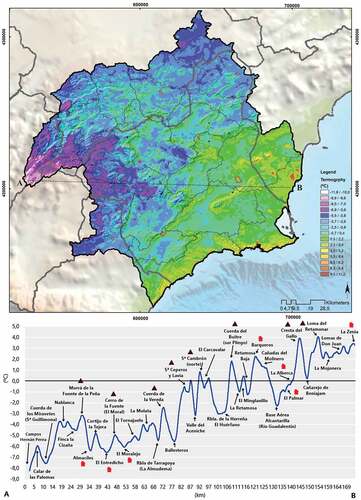
For a better visualization of the CAPs in the study area, as well as the thermal variability of the minimum temperatures during stable nights, thermal transects (reflected in Figure 7) can be made; these are very useful to describe the thermal irregularity in orographically rugged regions. The results are similar in the CAP and WAM areas. However, when considering only early mornings with NTI processes, the correlation of the combined VIIRS/MODIS LST product with altitude/temperature is not so high, although it is also important (R² of −0.89 and −0.81 in CAP areas and WAM, respectively) (Figure 8a and 8b).

Figure 7. Statistical correlation (Spearman test) between altitude (m) and temperature according to combined thermography (MODIS-VIIRS LST) in areas of: a) CAPs and b) WAM; c) average temperature per altitudinal range within CAPs and WAM, obtained with MODIS/VIIRS LST products. Solid green line show linear regression, dashed red line is nonparametric estimate of the mean, dashed blue line is nonparametric estimate of the variance, and blue shaded area is data-concentration ellipse.

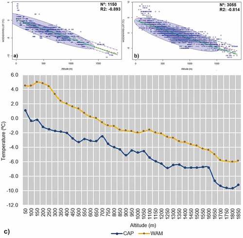
Figure 8. Average thermography of MODIS and VIIRS LST products across a thermal transect (A-B). Red symbols refer to population entities and brown triangles refer to mountain peaks.

Such high statistical correlation values indicate a robust statistical relevance, which corroborates the idea that the altitude of a CAP determines its temperature, being colder at higher altitudes. Inside the CAPs, the combined MODIS/VIIRS LST product (turquoise line) exhibits greater thermal variability according to the altitudinal range. Therefore, there is a greater influence of the CAPs, which is very well represented by the products analyzed. In addition, lower temperatures are seen at the altitude levels of 500, 900, 1250, and, especially, 1750 m.

However, for the WAM areas (Figure 9), excluding the NTI processes, and with a standard vertical thermal gradient (0.65°C/100 m), both lines follow a slightly altered evolution. Only the geographical areas at a lower altitude (<150 m), and located in coastal and pre-coastal zones, present temperatures lower than those at the altitude level of 150–200 m, due to the maritime influence. In addition, the combined MODIS/VIIRS LST product also reflects in much more detail the temperatures of mountainous areas, in orographically complex territories. Although the standard thermal gradient should result in lower temperatures at higher altitudes, the truth is that there are some exceptions – especially at 1100 m altitude, where a rise in temperature is appreciated with respect to the adjacent heights (1000 or 1200 m).

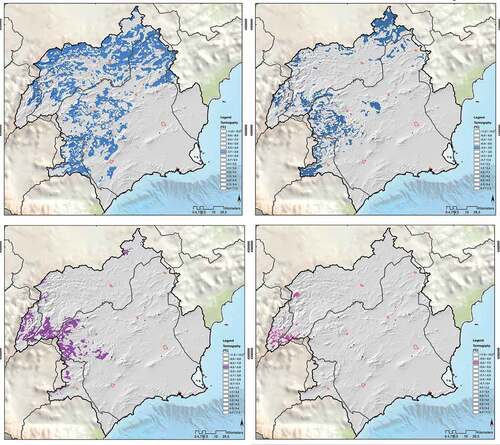
Figure 9. Temperature ranges with the MODIS and VIIRS LST combined product, where the coldest CAPs are identified.

With thermographies it is possible to identify the coldest inhabited nuclei in a territory, mainly due to the identification of CAPs. It is possible to identify municipal capitals and population entities (inhabited) (according to the Municipal Register, 2018). Thus, with reference to the municipal capitals, the coldest thermal extremes occur in Nerpio (Albacete) and Santiago de la Espada (Jaén), located at altitudes between 1100 and 1300 m, and in topographically depressed sectors. While, with temperatures that are 12/13°C higher, the least cold municipal centers are Águilas (Murcia) and Callosa del Segura (Alicante), located on the south coast of the Region of Murcia and in foothills of the medium reliefs of the Vega Alta del Segura, respectively.

High resolution thermographies in the study area: identification of CAPs at different scales

The combined product of the MODIS and VIIRS satellite images (LST) reflects, with a high resolution, the temperature distribution during stable early mornings (with NTI processes). With this, it is possible to identify the CAPs in each of the climatic regions generated; these are of high validity, especially for agricultural planning.

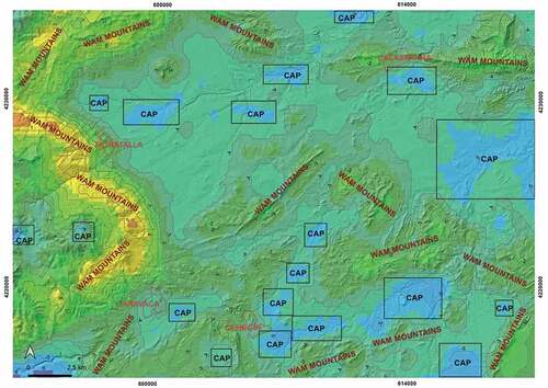
Figure 10 shows the identification of CAPs in an interior region of the study area. The CAPs identified have an area of at least 1 km² (Figure 10). A smaller size cannot be identified due to the spatial resolution of the analyzed product. Thermal differences of up to 8°C can be seen over a straight line distance of just 4 km, between the coldest CAPs and the orographically more rugged (more temperate) areas. The excellent spatial resolution makes it possible to identify the urban heat island effect in the inhabited municipalities of the study area, which have an average size of 1 to 1.5 km² and a population between 8000 and 25,000 inhabitants.

Figure 10. Spatial distribution of the temperatures estimated by the combination of the MODIS and VIIRS LST products. Identification of CAPs with high resolution thermography in the southeastern interior of Spain (province of Murcia).

Discussion

To map the nocturnal inversion phenomena (NTI) and the distribution of temperatures in a territory, a specific tool is required, such as satellite images. Due to the complexity of the spatial distribution of nighttime temperatures during stable early mornings (when CAPs form in valley bottoms), and the impossibility of maintaining a network of meteorological stations dense enough to identify the phenomenon well, thermographs are used; that is, thermal distributions derived from satellite bands.

When observational data are reduced on the air temperature at the earth’s surface, the surface temperature recovered by satellite is used. However, the spatial resolution of satellite-derived products must be taken into account, as they can be misleading on a local scale. On a fine scale, cold air drainage can induce a reversal of the temperature gradient with elevation. A higher correlation was found during the night on the fine scale (local; Collados‐Lara et al., 2021).

The MODIS and VIIRS LST products have the potential to provide excellent spatial estimates of LST at very high temporal (daily) and spatial (1000/750 m) resolution, all over the planet. The nocturnal analysis carried out here gave excellent results, with a better prediction for minimum temperatures (Tmin) than for maximum temperatures (Tmax) in the analysis of the MODIS LST products (Emamifar et al., 2013; Yang et al., 2017).

These statistical correlations are within the range of those found in the main investigations carried out previously, being similar to those of Neteler (2010), who found correlations between 0.70 and 0.98, as well as thermal differences of 0.5°C, between the temperatures of meteorological stations and those of MODIS LST in the central-eastern Alps (northeastern Italy). Also, the results indicate a significant correlation between LST and Ta with regression coefficients R² > 0.94/0.96 and Root Mean Square Error about 1.75/0.97°C of LSTd/Tmax and LSTn/Tmin, respectively similar to United Arab Emirates (Alqasemi et al., 2020).

The mean differences in the study area are between 2.4 and 3.8°C, although they are smaller in CAP areas (1.6 to 2.1°C). The validation results show that the daily minimum air temperature can be effectively recovered with the MODIS/VIIRS LST land surface products, as determined by Zhu et al. (2013).

In the Svalbard Islands (Norway) differences of 1.5 to 6.0°C in winters under clear sky conditions were found with MODIS LST, the surface temperatures being lower than those obtained with the products as we have also found (Westermann et al., 2012). The results obtained in the Maipo basin (Chile) also show a correct representation of the spatial and temporal distribution of the maximum and minimum temperatures for all types of surface (Bustos & Meza, 2015). In the westernmost region of Africa, Vancutsem et al. (2010) obtained high correlation coefficients between Ta and LST, with an R² of 0.86 in Botswana, 0.83 in Madagascar, and 0.69 in Eritrea. In northeast Vietnam simple multiple linear regression analysis was used, and high precision was achieved, with an R² of 0.88 (Noi et al., 2016). All these results are within the range calculated for our study area.

The results of recent years show that the spatio-temporal method yields good results in the production of LST products (MODIS – MYD11A1) in the Tibetan plateau (Zhou et al., 2017). Studies carried out on the European continent, specifically in the metropolitan area of Rome, yielded R² values between 0.87 and 0.93 for the nighttime product of MYD11A1 (Sismanidis et al., 2016), underlining that the MODIS LST product has provided correlations above 0.80 in most studies. In the work of Niclòs et al. (2018), the VIIRS product (LST) provided a good precision, of 0.4 K and 0.12 K, and R-RMSD values of 1.2 K and 1.1 K during the day and night, respectively, for all the coverages. In the present work, the MODIS and VIIRS LST products are tremendously homogeneous, with a correlation coefficient of 0.91 and a thermal difference of 0.4 K, although both underestimate the LST. Since they have almost the same statistical correlation with the surface temperatures (0.84 and 0.83, respectively), and a fairly small spatial resolution difference, the two products can be combined in a final thermography.

The accuracy is therefore better at night than during the daytime. In addition, the VIIRS product quality (LST) shows significant seasonality, with better performance in fall and winter than in spring and summer, key in the paper’s analysis. In addition, VIIRS, with a resolution of 750 m, and MODIS (1 km) were found to give excellent results, with differences of <0.5 K between the two (Hulley et al., 2017). The results indicate that the current VIIRS products (LST) yielded a very reasonable precision, with average biases of 0.36 K and −0.58 K and average RMSEs of 2.7 K and 1.5 K during the day and night, respectively (Liu et al., 2015; Niclòs et al., 2018). However, in the work of Li et al. (2014), three arid sites during the day and one arid surface site at night showed absolute biases greater than 1.5 K. Furthermore, these authors showed that the precision at night was much better than during the day: the daytime RMSEs were greater than 2 K for all four sites whereas the nighttime RMSEs were around 1 K.

The realization of the cartography proposed in this chapter supposes an advance in our knowledge of the territorial distribution of night temperatures during stable nights, as well as CAPs, which have been studied little through remote sensing, although they have been analyzed in the Balearic Islands, obtaining maps of the minimum air temperature (Jiménez et al., 2015), or Cerdanya Valley-Pyrenees (Martínez Villagrasa et al., 2016). It has also been used to simulate a persistent cold air pool event (PCAP) in the section of the valley of the river Arve around Passy in the French Alps. the study highlights the interaction between large-scale flow, tributary flows and the thermal structure of the PCAP (Arduini et al., 2020).

In recent years, remote sensing has become a first-rate methodological tool for many fields of climatology. The MODIS LST is considered one of the most suitable ways to recover the air surface temperature (Ta; Phan et al., 2019; Shen & Leptoukh, 2011). It has been used, during the last few years, to evaluate the diagnostic indicator of agricultural water use and crop stress (Xue et al., 2020), vegetation phenology such as the start (SOS) and end (EOS) of the growing season (Xu et al., 2020), potential TVX (Temperature-Vegetation Index) derived from the MODIS thermal images in order to estimate the minimum and maximum daily air temperatures in the city of Bangkok (Misslin et al., 2018), global coverage (Metz et al., 2014; Sobrino et al., 2020), spatial and temporal rates of change of MODIS-based daytime and nighttime LST for the last 19 years (Jaber & Abu-Allaban, 2020) and for the study of urban heat islands (ICU); for example, in Madrid (Allende et al., 2018).

The improvement of the minimum temperature surfaces, with the identification of nocturnal CAPs through satellite images, allows the improvement and capacity of the mesoscale temperature prediction.

Conclusions

The results of the statistical analysis show an especially good validation of the MODIS and VIIRS LST products, especially with the validations carried out using the surface temperatures (TN) of 219 meteorological stations in the study area. The statistical fits obtained with the combined MODIS and VIIRS LST product are high, the statistical correlation with the surface meteorological stations data having an R² of 0.87, with a total of 2579 and 3046 measurement points (very robust statistics). The spatial correlation is somewhat more important within the CAPs than in the zones outside the thermal inversion (WAM), R² being 0.76 and 0.75, respectively.

Although the main objective of this work was to analyze the spatial thermal distribution in the southeast of Spain during stable early mornings, the thermal differences found are not especially high, when comparing LST obtained using the MODIS/VIIRS (LST) products with air temperature (Ta) values from weather stations. The mean differences are between 2.4 and 3.8°C, although they are smaller in CAP areas (1.6 to 2.1°C). The standard deviation (SD), in general, is greater than 3.5 K, but it is less than 3 K in the interior valleys with formation of CAPs, so the recurrence of cold pools in certain places is very high.

Disclosure statement

No potential conflict of interest was reported by the author(s).

References

- Allende, F. A., Fernández, F. G., Rasilla, D. A., & Alcaide, J. M. (2018). Isla de calor nocturna estival y confort térmico en Madrid: Avance para un planeamiento térmico en áreas urbanas. Ciudad y Territorio Estudios Territoriales (CyTET), 50(195), 101–120. http://hdl.handle.net/10486/689801
- Alqasemi, A. S., Hereher, M. E., Al-Quraishi, A. M. F., Saibi, H., Aldahan, A., & Abuelgasim, A. (2020). Retrieval of monthly maximum and minimum air temperature using MODIS aqua land surface temperature data over the United Arab Emirates. Geocarto International, 1–18. https://doi.org/10.1080/10106049.2020.1837261
- Anderson, M. C., Kustas, W. P., Norman, J. M., Hain, C. R., Mecikalski, J. R., Schultz, L., & Gao, F. (2011). Mapping daily evapotranspiration at field to continental scales using geostationary and polar orbiting satellite imagery. Hydrology and Earth System Sciences, 15(1), 223–239. https://doi.org/10.5194/hess-15-223-2011
- Arduini, G., Chemel, C., & Staquet, C. (2020). Local and non‐local controls on a persistent cold‐air pool in the Arve River Valley. Quarterly Journal of the Royal Meteorological Society, 146(731), 2497–2521. https://doi.org/10.1002/qj.3776
- Barnes, W. L., Pagano, T. S., & Salomonson, V. V. (1998). Prelaunch characteristics of the moderate resolution imaging spectroradiometer (MODIS) on EOS-AM1. IEEE Transactions on Geoscience and Remote Sensing, 36(4), 1088–1100. https://doi.org/10.1109/36.700993
- Bolstad, P. V., Swift, L., Collins, F., & Régnière, J. (1998). Measured and predicted air temperatures at basin to regional scales in the southern Appalachian Mountains. Agricultural and Forest Meteorology, 91(3–4), 161–176. https://doi.org/10.1016/S0168-1923(98)00076-8
- Bustos, E., & Meza, F. J. (2015). A method to estimate maximum and minimum air temperature using MODIS surface temperature and vegetation data: Application to the Maipo Basin, Chile. Theoretical and Applied Climatology, 120(1–2), 211–226. https://doi.org/10.1007/s00704-014-1167-2
- Cao, C., Xiong, J., Blonski, S., Liu, Q., Uprety, S, S., & Weng, F. (2013). Suomi NPP VIIRS sensor data record verification, validation, and long‐term performance monitoring. Journal of Geophysical Research: Atmospheres, 118(20), 11–664. https://doi.org/10.1002/2013JD020418
- Chai, T., & Draxler, R. R. (2014). Root mean square error (RMSE) or mean absolute error (MAE)? Arguments against avoiding RMSE in the literature. Geoscientific Model Development, 7(3), 1247–1250. https://doi.org/10.5194/gmd-7-1247-2014
- Collados‐Lara, A. J., Fassnacht, S. R., Pulido‐Velazquez, D., Pfohl, A. K., Morán‐Tejeda, E., Venable, N. B., … Puntenney‐Desmond, K. (2021). Intra-day variability of temperature and its near-surface gradient with elevation over mountainous terrain: Comparing MODIS land surface temperature data with coarse and fine scale near-surface measurements. International Journal of Climatology, 41(S1), E1435–E1449. https://doi.org/10.1002/joc.6778
- Dodson, R., & Marks, D. (1997). Daily air temperature interpolated at high spatial resolution over a large mountainous region. Climate Research, 8(1), 1–20. https://doi.org/10.3354/cr008001
- Duan, S. B., Li, Z. L., Li, H., Göttsche, F. M., Wu, H., Zhao, W., & Coll, C. (2019). Validation of Collection 6 MODIS land surface temperature product using in situ measurements. Remote Sensing of Environment, 225, 16–29. https://doi.org/10.1016/j.rse.2019.02.020
- Emamifar, S., Rahimikhoob, A., & Noroozi, A. A. (2013). Daily mean air temperature estimation from MODIS land surface temperature products based on M5 model tree. International Journal of Climatology, 33(15), 3174–3181. https://doi.org/10.1002/joc.3655
- Flores, F., Arriagada, A., Donoso, N., Martínez, A., Viscarra, A., Falvey, M., & Schmitz, R. (2020). Investigation of a Nocturnal Cold-Air Pool in a Semiclosed Basin Located in the Atacama Desert. Journal of Applied Meteorology and Climatology, 59(12), 1953–1970. https://doi.org/10.1175/JAMC-D-19-0237.1
- Foster, C. S., Crosman, E. T., & Horel, J. D. (2017). Simulations of a cold-air pool in Utah’s Salt Lake Valley: Sensitivity to land use and snow cover”. Boundary-Layer Meteorology, 164(1), 63–87. https://doi.org/10.1007/s10546-017-0240-7
- Frei, C. (2014). Interpolation of temperature in a mountainous region using nonlinear profiles and non‐Euclidean distances. International Journal of Climatology, 34(5), 1585–1605. https://doi.org/10.1016/j.rse.2019.02.020
- González, S., & Garreaud, R. (2019). Spatial variability of near-surface temperature over the coastal mountains in southern Chile (38 S). Meteorology and Atmospheric Physics, 131(1), 89–104. https://doi.org/10.1007/s00703-017-0555-4
- Guillevic, P. C., Biard, J. C., Hulley, G. C., Privette, J. L., Hook, S. J., Olioso, A., & Csiszar, I. (2014). Validation of Land Surface Temperature products derived from the Visible Infrared Imaging Radiometer Suite (VIIRS) using ground-based and heritage satellite measurements. Remote Sensing of Environment, 154, 19–37. https://doi.org/10.1016/j.rse.2014.08.013
- Hachem, S., Allard, M., & Duguay, C. (2009). Using the MODIS land surface temperature product for mapping permafrost: An application to Northern Quebec and Labrador, Canada. Permafrost and Periglacial Processes, 20(4), 407–416. https://doi.org/10.1002/ppp.672
- Hillger, D. (2013). First-light imagery from Suomi NPP VIIRS. Bull. Amer. Meteorol. Society, 94(7), 1019–1029. https://doi.org/10.1175/BAMS-D-12-00097.1
- Hulley, G. C., Malakar, N. K., Islam, T., & Freepartner, R. J. (2017). NASA’s MODIS and VIIRS land surface temperature and emissivity products: A long-term and consistent earth system data record. IEEE Journal of Selected Topics in Applied Earth Observations and Remote Sensing, 11(2), 522–535. https://doi.org/10.1109/JSTARS.2017.2779330
- Hutchinson, K. D., & Cracknell, A. P. (2006). Visible infrared imager radiometer suite—A new operational cloud imager. Taylor & Francis.
- Jaber, S. M., & Abu-Allaban, M. M. (2020). MODIS-based land surface temperature for climate variability and change research: The tale of a typical semi-arid to arid environment. European Journal of Remote Sensing, 53(1), 81–90. https://doi.org/10.1080/22797254.2020.1735264
- Jarvis, `. C. H., & Stuart, N. (2001). A comparison among strategies for interpolating maximum and minimum daily air temperatures. Part II: The interaction between number of guiding variables and the type of interpolation method. Journal of Applied Meteorology, 40(6), 1075–1084. https://doi.org/10.1175/1520-0450(2001)0401075:ACASFI2.0.CO;2
- Jiménez, M. A., Ruiz, A., & Cuxart, J. (2015). Estimation of cold pool areas and chilling hours through satellite-derived surface temperatures. Agricultural and Forest Meteorology, 207, 58–68. https://doi.org/10.1016/j.agrformet.2015.03.017
- Jones, P., Jedlovec, G., Suggs, R., & Haines, S. (2004). Using MODIS LST to estimate minimum air temperatures at night. In 13th Conference on Satellite Meteorology and Oceanography (pp. 13–18). AMS Norfolk, VA.
- Justice, C. O., Román, M. O., Csiszar, I., Vermote, E. F., Wolfe, R. E., Hook, S. J., Tschudi, M., Wang, Z., Schaaf, C. B., Miura, T., Tschudi, M., Riggs, G., Hall, D. K., Lyapustin, A. I., Devadiga, S., Davidson, C., & Masuoka, E. J. (2013). Land and cryosphere products from Suomi NPP VIIRS: Overview and status. Journal of Geophysical Research: Atmospheres, 118(17), 9753–9765. https://doi.org/10.1002/jgrd.50771
- Katurji, M., & Zhong, S. (2012). The influence of topography and ambient stability on the characteristics of cold-air pools: A numerical investigation. Journal of Applied Meteorology and Climatology, 51(10), 1740–1749. https://doi.org/10.1175/JAMC-D-11-0169.1
- Langer, M., Westermann, S., Heikenfeld, M., Dorn, W., & Boike, J. (2013). Satellite-based modeling of permafrost temperatures in a tundra lowland landscape. Remote Sensing of Environment, 135, 12–24. https://doi.org/10.1016/j.rse.2013.03.011
- Lareau, N. P. (2014). The Dynamics of persistent cold-air pool breakup (Doctoral dissertation, Department of Atmospheric Sciences, University of Utah).
- Lee, Z. P. (2006). Remote sensing of inherent optical properties: Fundamentals, tests of algorithms, and applications. International Ocean Colour Coordinating Group (IOCCG).
- Lin, X., Zhang, W., Huang, Y., Sun, W., Han, P., Yu, L., & Sun, F. (2016). Empirical estimation of near-surface air temperature in China from MODIS LST data by considering physiographic features. Remote Sensing, 8(8), 629. https://doi.org/10.3390/rs8080629
- Li, H., Sun, D., Yu, Y., Wang, H., Liu, Y., Liu, Q., & Cao, B. (2014). Evaluation of the VIIRS and MODIS LST products in an arid area of Northwest China. Remote Sensing of Environment, 142, 111–121. https://doi.org/10.1016/j.rse.2013.11.014
- Liu, Y., Yu, Y., Yu, P., Göttsche, F., & Trigo, I. (2015). Quality assessment of S-NPP VIIRS land surface temperature product. Remote Sensing, 7(9), 12215–12241. https://doi.org/10.3390/rs70912215
- Martínez Villagrasa, D., Conangla Triviño, L., Simó, G., Jiménez Cortés, M. A., Tabarelli, D., Miró Cubells, J. R., & Cuxart Rodamillans, J. (2016). Cold-air pooling in the Cerdanya valley (Pyrenees). In EMS Annual Meeting abstracts.
- Metz, M., Rocchini, & Neteler, M, D. (2014). Surface temperatures at the continental scale: Tracking changes with remote sensing at unprecedented detail. Remote Sensing, 6(5), 3822–3840. https://doi.org/10.3390/rs6053822
- Minnett, P. J., Evans, R. H., Podestá, G. P., & Kilpatrick, K. A. (2014). Sea-surface temperature from suomi-NPP VIIRS: Algorithm development and uncertainty estimation. In Ocean Sensing and Monitoring VI. (Vol. 9111, pp. 91110C). International Society for Optics and Photonics. SPIE 9111, Ocean Sensing and Monitoring VI, 91110C. https://www.spiedigitallibrary.org/conference-proceedings-of-spie/9111/91110C/Sea-surface-temperature-from-Suomi-NPP-VIIRS--algorithm-development/10.1117/12.2053184.short?SSO=1
- Misslin, R., Vaguet, Y., Vaguet, A., & Daudé, É. (2018). Estimating air temperature using MODIS surface temperature images for assessing Aedes aegypti thermal niche in Bangkok, Thailand. Environmental Monitoring and Assessment, 190(9), 537. https://doi.org/10.1007/s10661-018-6875-0
- Mostovoy, G. V., King, R. L., Reddy, K. R., Kakani, V. G., & Filippova, M. G. (2006). Statistical estimation of daily maximum and minimum air temperatures from MODIS LST data over the state of Mississippi. GIScience & Remote Sensing, 43(1), 78–110. https://doi.org/10.2747/1548-1603.43.1.78
- Mutiibwa, D., Strachan, S., & Albright, T. (2015). Land surface temperature and surface air temperature in complex terrain. IEEE Journal of Selected Topics in Applied Earth Observations and Remote Sensing, 8(10), 4762–4774. https://doi.org/10.1109/JSTARS.2015.2468594
- Nalder, I. A., & Wein, R. W. (1998). Spatial interpolation of climatic normals: Test of a new method in the Canadian boreal forest. Agricultural and Forest Meteorology, 92(4), 211–225. https://doi.org/10.1016/S0168-1923(98)00102-6
- Neteler, M. (2010). Estimating daily land surface temperatures in mountainous environments by reconstructed MODIS LST data. Remote Sensing, 2(1), 333–351. https://doi.org/10.3390/rs1020333
- Niclòs, R., Pérez-Planells, L., Coll, C., Valiente, J. A., & Valor, E. (2018). Evaluation of the S-NPP VIIRS land surface temperature product using ground data acquired by an autonomous system at a rice paddy. ISPRS Journal of Photogrammetry and Remote Sensing, 135, 1–12. https://doi.org/10.1016/j.isprsjprs.2017.10.017
- Noi, P., Kappas, M., & Degener, J. (2016). Estimating daily maximum and minimum land air surface temperature using MODIS land surface temperature data and ground truth data in Northern Vietnam. Remote Sensing, 8(12), 1002. https://doi.org/10.3390/rs8121002
- Opazo, S., & Chuvieco, E. (2007). Utilización de productos MODIS para la cartografía de áreas quemadas. Revista de Teledetección, 27, 27–43.
- Phan, T. N., Kappas, M., Nguyen, K. T., Tran, T. P., Tran, Q. V., & Emam, A. R. (2019). Evaluation of MODIS land surface temperature products for daily air surface temperature estimation in northwest Vietnam. International Journal of Remote Sensing, 40(14), 5544–5562. https://doi.org/10.1080/01431161.2019.1580789
- Potter, C., & Alexander, O. (2019). Changes in vegetation cover and snowmelt timing in the Noatak national preserve of Northwestern Alaska estimated from MODIS and Landsat satellite image analysis. European Journal of Remote Sensing, 52(1), 542–556. https://doi.org/10.1080/22797254.2019.1689852
- Rajasekar, U., & Weng, Q. (2009). Urban heat island monitoring and analysis using a non-parametric model: A case study of Indianapolis. ISPRS Journal of Photogrammetry and Remote Sensing, 64(1), 86–96. https://doi.org/10.1016/j.isprsjprs.2008.05.002
- Schroeder, W., & Giglio, L. (2017). VIIRS/NPP thermal anomalies/Fire 6-Min L2 Swath 750m V001. In NASA EOSDIS Land Processes DAAC. https://doi.org/10.5067/VIIRS/VNP14.001
- Shapiro, S. L., Schwartz, G. E., & Bonner, G. (1998). Effects of mindfulness-based stress reduction on medical and premedical students. Journal of Behavioral Medicine, 21(6), 581–599. https://doi.org/10.1023/A:1018700829825
- Shen, S., & Leptoukh, G. G. (2011). Estimation of surface air temperature over central and eastern Eurasia from MODIS land surface temperature. Environmental Research Letters, 6(4), 045206. https://doi.org/10.1088/1748-9326/6/4/045206
- Sismanidis, P., Keramitsoglou, I., Bechtel, B., & Kiranoudis, C. (2016). Improving the downscaling of diurnal land surface temperatures using the annual cycle parameters as disaggregation kernels. Remote Sensing, 9(1), 23. https://doi.org/10.3390/rs9010023
- Sobrino, J. A., Julien, Y., & García-Monteiro, S. (2020). Surface temperature of the planet earth from satellite data. Remote Sensing, 12(2), 218. https://doi.org/10.3390/rs12020218
- Sun, D., & Pinker, R. T. (2003). Estimation of land surface temperature from a Geostationary Operational Environmental Satellite (GOES‐8). Journal of Geophysical Research: Atmospheres, 108(D11). https://doi.org/10.1029/2002JD002422
- Thornton, P. E., Running, S. W., & White, M. A. (1997). Generating surfaces of daily meteorological variables over large regions of complex terrain. Journal of Hydrology, 190(3–4), 214–251. https://doi.org/10.1016/S0022-1694(96)03128-9
- Vancutsem, C., Ceccato, P., Dinku, T., & Connor, S. J. (2010). Evaluation of MODIS land surface temperature data to estimate air temperature in different ecosystems over Africa. Remote Sensing of Environment, 114(2), 449–465. https://doi.org/10.1016/j.rse.2009.10.002
- Voinov, V. G., & Nikulin, M. S. (1993). Techniques for constructing Unbiased Estimators. In Unbiased Estimators and Their Applications (pp. 145–246). Springer.
- Wang, M., He, G., Zhang, Z., Wang, G., Wang, Z., Yin, R., Cui, S., Wu, Z., & Cao, X. (2019). A radiance-based split-window algorithm for land surface temperature retrieval: Theory and application to MODIS data. International Journal of Applied Earth Observation and Geoinformation, 76, 204–217. https://doi.org/10.1016/j.jag.2018.11.015
- Wan, Z., Hook, S., & Hulley, G. (2015). MYD11A1 MODIS/Aqua Land Surface Temperature/Emissivity Daily L3 Global 1km SIN Grid V006. NASA EOSDIS Land Processes DAAC. https://doi.org/10.5067/MODIS/MYD11A1.006
- Wan, Z., & Li, Z. L. (2010). MODIS land surface temperature and emissivity. Land Remote Sensing and Global Environmental Change (pp. 563–577). Springer. https://doi.org/10.1007/978-1-4419-6749-7_25
- Westermann, S., Langer, M., & Boike, J. (2012). Systematic bias of average winter-time land surface temperatures inferred from MODIS at a site on Svalbard, Norway. Remote Sensing of Environment, 118, 162–167. https://doi.org/10.1016/j.rse.2011.10.025
- Wolfe, R. E. (2006). MODIS geolocation. In Earth science satellite remote sensing (pp. 50–73). Springer.
- Xu, X., Du, H., Zhou, G., & Li, P. (2016). Method for improvement of MODIS leaf area index products based on pixel-to-pixel correlations. European Journal of Remote Sensing, 49(1), 57–72. https://doi.org/10.5721/EuJRS20164904
- Xue, J., Anderson, M. C., Gao, F., Hain, C., Sun, L., Yang, Y., Schull, M., Kustas, W. P., Torres-Rua, A., & Schull, M. (2020). Sharpening ECOSTRESS and VIIRS land surface temperature using harmonized Landsat-Sentinel surface reflectances. Remote Sensing of Environment, 251, 112055. https://doi.org/10.1016/j.rse.2020.112055
- Xu, X., Zhou, G., Du, H., Mao, F., Xu, L., Li, X., & Liu, L. (2020). Combined MODIS land surface temperature and greenness data for modeling vegetation phenology, physiology, and gross primary production in terrestrial ecosystems. Science of the Total Environment, 726, 137948. https://doi.org/10.1016/j.scitotenv.2020.137948
- Yang, Y., Cai, W., & Yang, J. (2017). Evaluation of MODIS land surface temperature data to estimate near-surface air temperature in Northeast China. Remote Sensing, 9(5), 410. https://doi.org/10.3390/rs9050410
- Yu, Y., Tarpley, D., Privette, J. L., Goldberg, M. D., Raja, M. R. V., Vinnikov, K. Y., & Xu, H. (2008). Developing algorithm for operational GOES-R land surface temperature product. IEEE Transactions on Geoscience and Remote Sensing, 47(3), 936–951. https://doi.org/10.1109/TGRS.2008.2006180
- Zängl, G. (2005). Formation of extreme cold-air pools in elevated sinkholes: An idealized numerical process study. Monthly Weather Review, 133(4), 925–941. https://doi.org/10.1175/MWR2895.1
- Zhong, S., Whiteman, C. D., Bian, X., Shaw, W. J., & Hubbe, J. M. (2001). Meteorological processes affecting the evolution of a wintertime cold air pool in the Columbia basin. Monthly Weather Review, 129(10), 2600–2613.
- Zhou, W., Peng, B., & Shi, J. (2017). Reconstructing spatial–temporal continuous MODIS land surface temperature using the DINEOF method. Journal of Applied Remote Sensing, 11(4), 046016. https://doi.org/10.1117/1.JRS.11.046016
- Zhu, W., Lű, A., & Jia, S. (2013). Estimation of daily maximum and minimum air temperature using MODIS land surface temperature products. Remote Sensing of Environment, 130, 62–73. https://doi.org/10.1016/j.rse.2012.10.034