Exploring evolutionary-tuned autoencoder-based architectures for fault diagnosis in a wind turbine gearbox

ABSTRACT

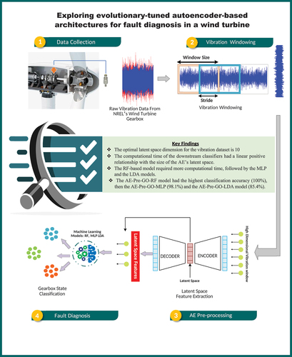
Vibration-based fault diagnosis from rotary machinery requires prior feature extraction, feature selection, or dimensionality reduction. Feature extraction is tedious, and computationally expensive. Feature selection presents unique challenges intrinsic to the method adopted. Nonlinear dimensionality reduction may be achieved through kernel transformations, however there is often a trade-off in information to achieve this. Given the above, this study proposes a novel autoencoder (AE) pre-processing framework for vibration-based fault diagnosis in wind turbine (WT) gearboxes. In this study, AEs are used to learn the features of WT gearbox vibration data while simultaneously compressing the data, obviating the need for costly feature engineering and dimensionality reduction. The effectiveness of the proposed framework was evaluated by training genetically optimized linear discriminant analysis (LDA), multilayer perceptron (MLP), and random forest (RF) models, with the AE’s latent space features. The models were evaluated using known classification metrics. The results showed that the performance of the models depends on the size of the AE’s latent space. As the size of the AE’s latent space increased, the quality of features extracted improved until a plateau was observed at a latent space dimension of 10. The AE pre-processed genetically optimized RF, MLP, and LDA models, designated AE-Pre-GO-RF, AE-Pre-GO-MLP, and AE-Pre-GO-LDA, were evaluated for accuracy, sensitivity, and specificity in the classification of seven (7) gearbox fault conditions. The AE-Pre-GO-RF model outperformed its counterparts, scoring 100% for all evaluated metrics, though with the longest training time (239.50 sec). Comparable results were found comparing this study with similar investigations involving traditional vibration processing techniques. More so, it was established that effective fault diagnosis of the WT gearbox can be achieved through manifold learning with AEs without expensive feature engineering.

Graphical Abstract

KEYWORDS:

• Autoencoders
• gearbox fault diagnosis
• feature extraction
• vibration signals
• wind turbine

1. Introduction

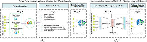
Vibration-based condition monitoring of the wind turbine (WT) gearbox [1] has gained significant attention due to its numerous benefits including the fact that it is noninvasive, reliable, cost effective and makes for early fault detection [2–4]. Several studies have employed vibration data for fault recognition in WT gearboxes [5–7]. The vibration signals are pre-processed before being fed to a Machine learning (ML) model [8]. The pre-processing of vibration data can be achieved in a few different ways; however, they can generally be grouped into two categories: (1) Feature extraction – feature selection (FE-FS) vibration pre-processing strategy and (2) Feature extraction – dimensionality reduction (FE-DR) vibration pre-processing strategy. In the FE-FS strategy, feature extraction is performed first, followed by feature selection. Feature extraction begins by segmenting the vibration signal into equal time windows [9]. To capture the essential characteristics of the vibration signal, the window size must be sufficiently large [10]. This generates a high-dimensional dataset. Essential statistical features are then extracted from each window using appropriate formulars [11]. This way, the original high-dimensional dataset is represented using fewer dimensions that together account for a significant portion of the variance in the original data [12].

Feature extraction from windowed vibration signals is performed in time domain, frequency domain, and/or time-frequency domain [13–15]. In time domain, statistical features are computed directly from the segmented vibration signal. Typical functions employed for this purpose include: signal mean, peak to peak, kurtosis, standard deviation, entropy, and so on [16,17]. In frequency domain, feature extraction begins by converting the raw vibration waveform into a spectrum through fast Fourier Transform [18]. Thereafter, frequency domain features, including maximum power spectral density, mean frequency, and mean power spectral density, are computed from the vibration spectrum [19,20]. In time-frequency domain [21], various techniques such as short-time Fourier transform (STFT), discrete wavelet transforms (DWT), empirical mode decomposition (EMD), two-level adaptive chirp mode decomposition, swarm decomposition, and so on are used to decompose the vibration signal [22–26]. To mine all the essential patterns in vibration data, a typical feature engineering process extracts multiple features in multiple domains. This results in a high-dimensional feature set with multicollinearity among the extracted features. Thus, feature extraction is often followed by feature selection.

‘Feature selection’ selects a subset of features from the original feature set. The goal of feature selection is to generate a low-dimensional feature subset from the original feature space while preserving the original feature’s intuitive interpretation. During feature selection, redundant features are eliminated so that the final feature set has a minimal correlation with one another. Tang et al. [27] employed a time-frequency domain approach for vibration-based fault detection in a WT gearbox. The gearbox vibration signals were first transformed into time-frequency domain using complete ensemble empirical mode decomposition with adaptive noise (CEEMDAN). Thereafter, some statistical characteristics were derived from the signals. Feature selection was then performed using recursive feature elimination. The final feature set was used to train an extreme learning machine for fault classification in the WT gearbox. The proposed model achieved 99.6% classification accuracy for 10 different gearbox fault conditions. Other WT gearbox fault detection studies employing the FE-FS vibration pre-processing strategy can be found in the review by [28].

Feature selection techniques are grouped into embedded methods, wrapper methods, and filter methods [28]. Filter methods perform feature selection based on the intrinsic information content of the feature subset. They are employed independent of an external machine-learning model. Embedded techniques select the features as a part of the model-building procedure. Wrapper techniques implement feature selection by assigning scores to individual feature subsets with the help of a predictive model [29]. The features with the highest scores are finally selected. Wrapper methods employ different strategies, including recursive feature elimination, sequential forward selection, and backward elimination. Although several studies have employed the FE-FS vibration pre-processing strategy; this approach has a number of pertinent drawbacks. Wrapper methods for instance are constrained by their high computational cost and likelihood of overfitting. Embedded approaches require significant computational resources for a high dimensional feature space [30]. Filter techniques ignore feature dependencies, which typically leads to poor performance after training with the selected feature-set.

The FE-DR strategy begins with feature extraction, like its counterpart. However, dimension reduction is performed subsequent to feature extraction. Dimensionality reduction algorithms, in contrast to feature selection algorithms, generate an entirely new set of features by mapping the original high-dimensional feature set to a low-dimensional feature space. After the mapping, the correlation among the features in the data is removed. Frequently, the new feature set lacks tangible meaning or interpretation. Wang et al. [28] grouped dimensionality reduction techniques into linear techniques like principal component analysis (PCA) and non-linear techniques like kernel principal component analysis (KPCA). Like the FE-FS strategy, the FE-DR strategy also has notable limitations. Linear dimensionality reduction techniques for instance fail to identify essential non-linear data patterns in the vibration signal, resulting in diminished model performance [31]. Nonlinear kernel-based techniques, employ non-linear kernel mapping functions to project the extracted features into a higher dimensional feature space, however, there is often a trade-off in information loss to achieve these transformations. To remedy these shortcomings, we turn to a class of methods known as ‘manifold learning.’

‘Manifold learning’ is a nonlinear dimensionality reduction technique that seeks to uncover the intrinsic relationships between observations in a high-dimensional space on the assumption that they lie in a limited part of the space – typically a manifold embedded in the larger space [32]. By uncovering these patterns, these learning algorithms discover low-dimensional representations of the original data. Due to its wide range of application in domains such as pattern recognition, biometrics, data mining, visualization, and function approximation, manifold learning has garnered considerable interest among machine learning researchers. Manifold-learning algorithms include Isometric mapping (IsoMap), Locally Linear Embedding (LLE), t-distributed Stochastic Neighbour Embedding (t-SNE), Laplacian Eigenmaps, Multi-dimensional Scaling (MDS), and Autoencoders [33]. The conventional vibration processing framework proceeds in two stages. This approach is associated with a costly feature extraction, then feature selection or dimensionality reduction. By employing autoencoders however, we can maximize model effectiveness while minimizing the challenges presented by the conventional vibration pre-processing techniques.

Autoencoders (AE) are unsupervised neural network networks trained to capture the most crucial elements of an input data with the goal of learning a lower-dimensional representation of the data, generally for dimensionality reduction [34]. As we proceed from the input layer to the output layer of an AE, the number of nodes decrease, forming the shape of a funnel. A classical AE is composed of three primary components: the encoder, the bottleneck and the decoder [35]. The encoder consists of a group of neural networks that condense the model’s input into a compact area known as the bottleneck. The bottleneck is a low-dimensional feature-space imposed on the neural network architecture to achieve manifold learning. The function of the bottleneck is to limit the amount of data that can transverse the network, forcing a learnt compression of the input data [36]. The decoder consists of a sequence of up-sampling modules that help in reconstructing the input from its latent features [34]. Autoencoders are widely applied for different purposes including manifold learning, anomaly detection, image denoising, image compression, image generation and missing value importation.

In the WT research space, the application of AE has centered on anomaly detection from wind turbine SCADA data. Zhang et al. [37] employed long-short-term memory-based stacked denoising AEs and XGBoost for anomaly detection in a WT. The anomaly detection threshold was established with a 99.7% confidence interval for the distribution curve fitted by kernel density estimation, and the Mahalanobis distance was estimated based on the reconstruction errors. The results of the study validate the efficacy of the proposed approach in identifying anomalies in operational WTs. Albeit no prior research has employed AE for manifold learning of vibration data in the wind turbine research space, several scholars have employed the model in other domains for manifold learning with laudable results. For instance [38], employed sparse autoencoder for pre-processing acoustic signals for fault detection and classification in internal combustion engines. Unsupervised features learned from the acoustic signals by the autoencoder are employed to train a SoftMax classifier. The approach enhanced classification performance, achieving an accuracy of 98.9% with limited training data. Mishra et al. [39] proposed an autoencoder pre-processing strategy for intelligent fault detection in an elevator. Non-linear fault features learned from the vibration data by the autoencoder trained a random forest classifier. The model achieved 100% fault detection accuracy, outperforming conventional feature extraction-based models.

Vibration condition monitoring stands at the heart of WT condition monitoring as vibration anomalies could result in severe damage to the multi-billion-dollar wind turbine system. Considering the criticality of the WT gearbox, effort is ongoing toward developing more effective models with near-zero error to forestall the effect of mis-classification and consequentially minimize maintenance costs. Central to this objective is the choice of an effective strategy for pre-processing the vibration signal. The traditional pre-processing approach performs feature selection or dimensionality reduction after a feature extraction process. However, these processes have been observed to suffer from significant limitations [40]. Feature extraction from vibration data is tedious, requiring a significant amount of time and computational resources [41]. Also, feature selection presents unique challenges intrinsic to the feature selection method employed. For instance, filter methods employed in [42,43] evaluate each feature independently, using a univariate approach, ignoring feature dependencies; this frequently results in poor performance after training with the chosen feature-set [42]. Wrapper methods of feature selection on the other hand [44,45] are constrained by their high computational cost and likelihood of overfitting [30,40]. Similarly, studies have showed that embedded approaches [42,46,47] require significant computational resources for a high dimensional feature space. To address these limitations, some studies have adopted dimensionality reduction approach as opposed to feature selection. However, these also suffers unique difficulties. For instance, linear dimensionality reduction techniques such as principal component analysis fail to identify essential non-linear data patterns in the vibration signal, resulting in diminished model performance [31,48–50]. The transformation process in nonlinear kernel based techniques scarcely occur without information loss [51]. These limitations of the existing vibration pre-processing strategies motivate the implementation of AEs. Unlike conventional approaches, AEs do not require prior feature extraction. AEs employ a novel approach called ‘manifold learning’ to transform the input data from a high-dimensional space to a low-dimensional space while retaining the nonlinear patterns present in the original dataset. Although AEs have been employed for manifold learning with high success rates across a multitude of domains, they have not been employed for manifold learning of vibration signals in the wind turbine space. This study intends to bridge this gap. Employing the autoencoder pre-processing strategy for WT condition monitoring promises to benefit wind farm operators in achieving more accurate fault diagnosis. This will increase WT system availability toward meeting energy demand and power purchase agreements at the strategic level. In light of the above, this study proposes an autoencoder vibration pre-processing framework for multi-fault diagnosis in WT gearboxes. In brief, the study (i) implements a pre-processing strategy for vibration data based on AE; (ii) evaluates the strategy by training a linear discriminant analysis (LDA), multilayer perceptron (MLP), and random forest (RF) model with the pre-processed vibration data; (iii) optimizes the models with a genetic algorithm; (iv) investigates the effect of the size of the AE’s latent space on the performance and computational time of the machine-learning models; (v) compares the study results with analogous studies employing traditional vibration pre-processing strategies. While this section provides a background to the study, section 2 provides the theoretical background of concepts, section 3 presents a discussion of findings and section 4 concludes the study.

2. Theoretical background

This section provides the theoretical framework for each concept in this study as well as the mathematical framework for the proposed models. The study follows synopsis as shown in Figures 1(a,b). While Figure 1(a) summarizes the traditional pre-processing approach employed in vibration-based fault diagnosis, Figure 1(b) presents the proposed AE pre-processing framework.

Figure 1. Wind turbine gearbox vibration-based fault diagnosis: (a) Traditional vibration pre-processing framework (b) Autoencoder vibration pre-processing framework.

2.1. Dataset description

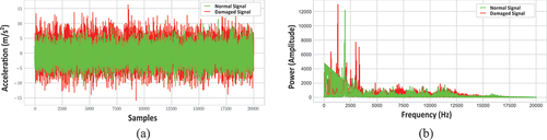
The study used NREL’s Vibration Condition Monitoring Benchmarking Dataset to validate the proposed models. The dataset was collected from two identical WT planetary gearboxes. A low-speed planetary stage, intermediate-speed stage, and high-speed stage make up each gearbox. The overall gear ratio of the gearboxes is 1:81.49. Different gearbox subcomponents used different bearings and gear elements based on loading and service requirements. The first gearbox’s internal bearings and gears were damaged during a wind farm test. Accelerometers were put on the damaged gearbox at the NREL lab to record vibrations. The vibration signals were sampled at 40 kHz under regulated loads. The damaged gearbox was then disassembled for analysis. After failure analysis, seven faults were found. Accelerometers were mounted at identical positions on the second, undamaged gearbox as on the damaged gearbox, and normal vibration data was collected. Ten groups of one-minute MATLAB (.MAT) files were retrieved from the healthy and damaged gearboxes. The high-speed shaft rotated at 1800 rpm and the main-shaft at 22.09 rpm. The intermediate speed shaft bearing’s damaged and normal vibration waveforms are shown in Figure 2(a,b). The damaged and normal vibration spectrum of the same bearing is shown in Figure 3(a,b). Lastly, Figure 4 depicts the waveform (a) and spectrum (b) of the bearing’s normal vibration signal superimposed on the damaged.

Figure 2. Vibration waveform of the intermediate speed shaft bearing: (a) Damaged signal (b) Normal signal.

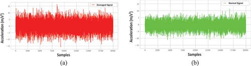
Figure 3. Vibration spectrum of the intermediate speed shaft bearing: (a) Damaged signal (b) Normal signal.

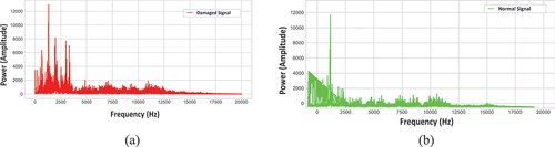
Figure 4. The waveform (a) and spectrum (b) of the intermediate speed shaft bearing’s normal vibration signals superimposed upon the damaged.

2.2. Vibration pre-processing with autoencoders

2.2.1. Autoencoders

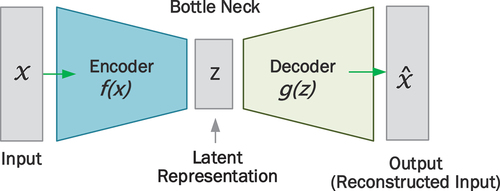
Autoencoders are unsupervised learning algorithms that modify their learnable weights to reconstruct input data from a latent low-dimensional space such that the output is identical to the input [52]. A typical AE is composed of three primary components: the encoder, the bottleneck and the decoder (Figure 5). The encoder consists of a group of neural networks that condense the model’s input into a compact area known as the bottleneck [35]. The bottleneck is a low-dimensional feature-space imposed on the neural network architecture to achieve manifold learning. The function of the bottleneck is to limit the amount of data that can transverse the network, forcing a learnt compression of the input data [36]. The decoder consists of a sequence of up-sampling modules that help in reconstructing the input from its latent features [34].

Figure 5. Schematic representation of a standard autoencoder model.

Given an input, x, the encoder transforms the input to a latent representation, z as follows:

(1) $\mathit{z}=\mathit{\phi }\left(\mathit{Wx}+\mathit{b}\right)$(1)

Where the parameter W is the encoder’s matrix of weights, b is a bias vector and φ is the encoder network’s activation function. The decoder network then transforms the latent space representation z to the output $\hat{x}$ as follows:

(2) $\hat{x}=\mathit{g}\left(\mathit{z}\right)=\mathit{\sigma }\left(\mathit{W}{ }^{\mathrm{\prime }}\mathit{z}+\mathit{b}{ }^{\mathrm{\prime }}\right)$(2)

Where the parameter, $\mathit{\sigma }$ is the decoder network’s activation function, $\mathit{b}{ }^{\mathrm{\prime }}$ is the decoder network’s bias vector and $\mathit{W}{ }^{\mathrm{\prime }}$ represents the weight matrix of the decoder network. The objective of training an AE is to produce an output as identical as possible to the original input. The reconstruction loss for a standard AE is depicted by the L1 loss (norm loss), given as:

(3) $\mathit{L}1=\left|\mathit{x}-\hat{x}\right|$(3)

Where $\hat{x}$ represents the predicted output and x represents the ground truth. The optimization equation of a standard autoencoder is given as follows:

(4) $\underset{\mathit{\theta }}{{\mathit{J}}_{\mathit{AE}}=\mathrm{minL}}\left(\mathit{x},\hat{x}\right)=\frac{1}{2\mathit{N}}\sum _{\mathit{i}=1}^N\parallel x_i-f_{\theta }\left(x_i\right){\parallel }^2$(4)

Where $\mathit{\theta }=\left[\mathit{W},\mathit{b},\mathit{W}{ }^{\mathrm{\prime }},\mathit{b}{ }^{\mathrm{\prime }}\right]$ denote the parameters of a standard autoencoder, the $\mathit{i}$-$\mathit{th}$ training sample is denoted by the parameter $x_i$, and the number of training samples by N. As there is no explicit regularization term in a standard AE, the only way to guarantee that the model isn’t memorizing the input data is to make the bottleneck sufficiently small [34].

2.2.2. Autoencoder vibration pre-processing framework

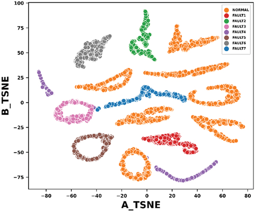
This study employed AEs to pre-process the gearbox vibration data. The raw vibration signals for the various gearbox fault conditions were partitioned into overlapping sliding windows of 1000 samples with a stride of 500 (Figure 6). The two-dimensional t-SNE (t-distributed stochastic neighbor embedding) scatter plot of the windowed vibration data is presented in Figure 7. Each window was fed to an AE model with fully connected (dense) layers. After training the AE model, the latent space (learned representation of the input data at the bottle neck) was extracted and given as input features to select conventional ML models for fault classification. To investigate the impact of the size of the latent space dimension on the quality of the features learned, different AE models with different latent space dimensions (2, 3, 5, 7, 10, 15 and 20) were employed in the study.

Figure 6. Autoencoder latent space feature extraction process.

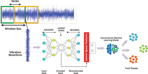
Figure 7. Two-dimensional t-TSNE scatter plot of a window of the vibration data.

The architectures of the different AE models are presented in Table 1. The autoencoder models were built on the conventional autoencoder model depicted in Figure 8. The layer and activation function were kept constant. Seven (7) different architectures were experimented to understand the effect of the latent space dimension on the quality of features extracted as evidenced by the performance of the downstream classifiers.

Figure 8. Architecture of a typical autoencoder model.

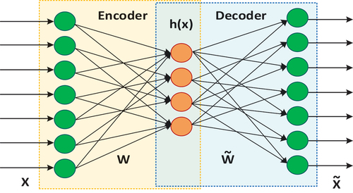
Table 1. The experimented Autoencoder model architectures.

Layer type	Dense
Activation function	Rectified Linear Unit (ReLU)
Model	Latent space dimension	Numbers of Neuron
1	2	500	250	100	50	20	10	2	10	20	50	100	250	500
2	3	500	250	100	50	20	10	3	10	20	50	100	250	500
3	5	500	250	100	50	20	10	5	10	20	50	100	250	500
4	7	500	250	100	50	20	10	7	10	20	50	100	250	500
5	10	500	250	100	50	20	10			20	50	100	250	500
6	15	500	250	100	50	20	15			20	50	100	250	500
7	20	500	250	100	50	20					50	100	250	500

The hyperparameter used in training the AE models are presented in Table 2.

Table 2. The Autoencoder model training hyperparameters.

Parameter Name	Value
Number of epochs	5
Batch size	100
Optimizer	Adam
Loss	Mean absolute error (MAE)
Learning rate	0.001

To investigate the effectiveness of the proposed AE vibration pre-processing strategy, the AE features were fed to three standard ML models for fault classification. They include LDA, MLP and RF model. The model development process is discussed in the section that follows.

2.3. Model development

2.3.1. Theory of the machine learning models

(a) Linear discriminant analysis

Linear Discriminant Analysis (LDA) is a parametric ML algorithm with a linear decision boundary, generated by fitting class conditional probability densities to a dataset using Bayes’ rule [53]. If all classes share the same covariance matrix, the model fits each class with a Gaussian density. Finding the linear combination of features that best distinguishes the classes in a dataset enables classification. This is achieved by projecting the data into a space with lower dimensions that maximizes class separation. LDA assumes that the data follows a Gaussian distribution and that the covariance matrices of all classes are identical [54]. First, the between-class variance is computed, then the within-class variance is computed, and lastly a lower-dimensional space is designed to maximize the between-class variance and minimize the within-class variance [55]. Let the between-class scatter matrix be ${\mathrm{S}}_b$ and the within-class scatter matrix be ${\mathrm{S}}_w$, then:

(5) ${\mathbf{S}}_{\mathbf{b}}=\frac{1}{N}\sum _{\mathit{i}=1}^c{N}_i\left({\bar{\mathbf{X}}}_{\mathit{i}}-\bar{\mathbf{X}}\right){\left({\bar{\mathbf{X}}}_{\mathit{i}}-\bar{\mathbf{X}}\right)}^{\mathit{T}}$(5)

And

(6) ${\mathbf{S}}_{\mathbf{w}}=\frac{1}{N}\sum _{\mathit{i}=1}^c\sum _{\mathit{s}=1}^{N_i}\left({\mathbf{X}}_s^i-{\bar{\mathbf{X}}}_{\mathit{i}}\right){\left({\mathbf{X}}_s^i-{\bar{\mathbf{X}}}_{\mathit{i}}\right)}^{\mathit{T}}$(6)

Linear discriminant analysis solves the optimization problem below [56]:

(7) $\underset{W}{max}\frac{\mathit{tr}\left({\mathbf{W}}^T{\mathbf{S}}_b\mathbf{W}\right)}{\mathit{tr}\left({\mathbf{W}}^T{\mathbf{S}}_w\mathbf{W}\right)}$(7)

Where tr(.) and (.)^T are respectively the trace operation and transposition of a matrix.

The optimal solution to the optimization problem in (7), $\mathrm{W}=\mathit{\hspace{0.17em}}\left({\mathrm{W}}_1,\dots ,{\mathrm{W}}_d\right)$ can be obtained from the generalized problem:

(8) ${\mathbf{S}}_{\mathbf{b}}\mathbf{w}=\mathit{\lambda }{\mathbf{S}}_{\mathbf{w}}\mathbf{w}$(8)

Where λ ≠ 0. If ${\mathrm{S}}_w$ is non-singular, then W is given by the first d largest eigenvalues of (${\mathrm{S}}_w$)⁻¹S_b.

(b) Multilayer perceptron (MLP)

Artificial neural networks (ANNs) are ML models with the same computational structure and behavior as biological neurons. The enormously complex, non-linear, parallel distributed structure of a neural network is what gives it its computational capacity [57]. Neural networks take in data, learn patterns in the data and predict the output for a new set of comparable data [58]. Three interconnected nonlinear processing units comprise a neuron: an input layer, one or more hidden layers, and an output layer [59]. Input features are received by the input layer. The hidden layer is where calculations on the input features are conducted [57]. The multilayer perceptron (MLP) is an artificial feed-forward neural network. In the latter, information moves only forward, from input nodes to output nodes via any hidden nodes. Feed-forward MLPs are devoid of cycles and loops. Traditional MLPs typically consist of no more than three layers; beyond three layers, the MLP transforms into a deep neural network [60]. The simple MLP has several advantages, including its simplicity of implementation, superior performance, and shorter training time. Among other algorithms, the back-propagation (BP) algorithm and the Levenberg-Marquardt algorithm are the most common MLP learning algorithms [61]. In back propagation, the neural network receives input features at the input layer. The inputs are each multiplied by the weights associated with their channel; a bias is added to the result and passed to an activation function, typically the rectified linear unit (ReLU) activation function (eq. 9).

(9) $\mathit{f}\left(\mathit{z}\right)=\left\{\begin{array}{c}0\mathit{for}\mathit{z}<0\\ \mathit{z}\mathit{for}\mathit{z}\ge 0\end{array}\right.$(9)

If the output of the activation function is up to a predefined threshold, the neuron fires and the result is passed to the neurons in the next layer. This way, data is propagated through the network, this is called forward propagation. In multiclassification problems, the output of the last hidden layer of the neural network is passed through a SoftMax activation function (eq. 10), which produces a vector of predicted probabilities over the input classes.

(10) $f_i\left(\mathit{z}\right)=\frac{{\mathit{e}}^{\mathit{zi}}}{{\sum }_{j=1}^j{e}^{\mathit{zj}}}$(10)

The output is compared with the actual value. The calculated error indicates the magnitude and direction of change required to reduce the error. This information is then propagated backwards to adjust the weight of the neurons. This is called back-propagation. The cycle continues until the error is as small as possible [58]. In multiclassification problems (which is the focus of this study), the loss function employed is the categorical cross-entropy (CE) loss, given as:

(11) $\mathit{CE}=-\sum _{\mathit{i}=1}^{\mathit{I}=\mathit{n}}{y}_i.log\left({\hat{y}}_{\mathit{i}}\right)$(11)

Where $y_i\mathit{and}{\hat{y}}_{\mathit{i}}$ are respectively the actual and predicted outputs.

(c) Random forest model

Random forest is an ensemble learning algorithm that employs multiple decision trees as base learners [62]. A decision tree is comprised of decision nodes, leaf nodes, and a root node [63,64]. A decision tree algorithm divides the training dataset into branches that further divide into additional branches. This process continues until a leaf node that cannot be further subdivided is reached. At a given non-leaf node, each decision tree in an ensemble selects the optimal division among the randomly selected candidate feature subsets. Random forest operates on the bootstrap aggregation principle, also known as bagging [64]. Bagging generates a number of new training sets by sampling the original training set with replacement and combining the results of trees fitted `[65].

Suppose we have a set of training vectors $x_i\in \mathit{\hspace{0.17em}}{R}^n,\mathit{\hspace{0.17em}}\mathit{i}=1,\dots ,\mathit{\hspace{0.17em}}\mathit{l}\mathit{\hspace{0.17em}}$ and a set of label vectors, $\mathit{y}\in \mathit{\hspace{0.17em}}{R}^l$, a decision tree divides the feature space iteratively in such a way that samples with related labels or target values are grouped together. Suppose the data at node m, has n samples and is represented by Q_m. Then for each individual split $\mathit{\theta }=\mathit{\hspace{0.17em}}(\mathit{j},\mathit{\hspace{0.17em}}{t}_m)$ consisting of a feature, j and a threshold, t_m, divide the data into two subsets: $Q_m^{\mathit{left}}\left(\mathit{\theta }\right)$ and $Q_m^{ri\mathrm{ght}}\left(\mathit{\theta }\right)$ subsets, where:

$Q_m^{\mathit{left}}\left(\mathit{\theta }\right)=\mathit{\hspace{0.17em}}\left\{\left(\mathit{x},\mathit{\hspace{0.17em}}\mathit{y}\right)|x_j\le \mathit{\hspace{0.17em}}{t}_m\mathit{\hspace{0.17em}}\right\}\mathit{\hspace{0.17em}}$

and

$Q_m^{ri\mathrm{ght}}\left(\mathit{\theta }\right)=\mathit{\hspace{0.17em}}{Q}_m\mathit{\hspace{0.17em}}\mathrm{\setminus }{Q}_m^{\mathit{left}}\left(\mathit{\theta }\right)$

The quality of an individual split of node m is subsequently calculated by means of an impurity function or loss function $\mathit{H}()$, the choice depends on whether the task at hand is a classification or regression problem. We define:

(12) $\mathit{G}\left(Q_m,\mathit{\hspace{0.17em}}\mathit{\theta }\right)=\mathit{\hspace{0.17em}}\frac{n_m^{l\mathrm{eft}}}{n_m}\mathit{H}\left(Q_m^{\mathit{left}}\left(\mathit{c}\right)\right)+\mathit{\hspace{0.17em}}\frac{n_m^{r\mathrm{ight}}}{n_m}\mathit{H}\left(Q_m^{ri\mathrm{ght}}\left(\mathit{\theta }\right)\right)$(12)

The parameters which minimize the impurity are chosen as:

${\theta }^{\ast }=\mathit{argmi}{n}_{\theta }\mathit{G}\left(Q_m,\mathit{\hspace{0.17em}}\mathit{\theta }\right)$

Iterate for subsets $Q_m^{\mathit{left}}\left({\theta }^{\ast }\right)$ and $Q_m^{ri\mathrm{ght}}\left({\theta }^{\ast }\right)$ until the maximum permissible depth is attained, that is $n_m<\mathit{\hspace{0.17em}}\mathit{mi}{n}_{\mathit{samples}}\mathit{\hspace{0.17em}}$ or $n_m=\mathit{\hspace{0.17em}}1.$

The random forest algorithm has found widespread application in numerous fields owing to its simple structure and superior performance compared to other ML algorithms [64].

2.3.2. Model development with LDA, MLP and RF

The scripts for the models were written in Python, installed on a laptop PC with a 12th Generation Intel Core i7 multi-core microprocessor, 32 GB of RAM and 1 TB of solid-state drive. The study employed 70% of the dataset for training the models, 15% for validation, and 15% for testing. The AE latent space features extracted were used to train three conventional ML algorithms including LDA, MLP and RF model. The hyperparameters of the models were optimized using Genetic Algorithm. Details of the hyperparameter optimization process are discussed in section 2.4.

2.4. Hyperparameter optimization with genetic algorithm

2.4.1. Genetic algorithm

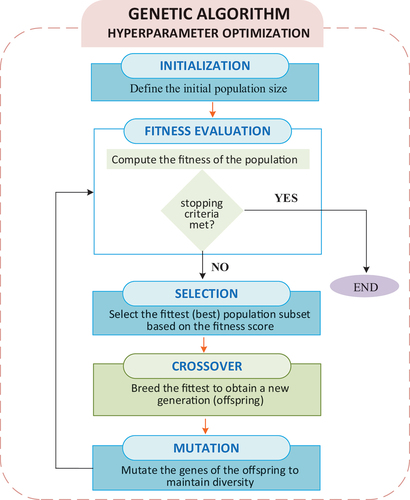
The recent years have seen increased application of evolutionary algorithms as optimization techniques for intelligent condition monitoring models [66,67]. Their ability to search for near-optimal solutions to both single- and multi-objective problems in a larger search space has made them increasingly relevant [67]. Common evolutionary algorithms include particle swarm optimization (PSO), artificial bee colony (ABC), genetic algorithm (GA) and so on [68]. Among these algorithms, GAs have received particular attention due to their many benefits including, increased search speed thanks to parallelism, a larger search space, the capacity to optimize for several objectives simultaneously, a probabilistic optimization strategy, and the discovery of near-optimal solutions [68]. Genetic algorithms are adaptive heuristic bio-inspired search algorithms [69], they model the principle of survival of the fittest [70]. Genetic algorithms mimic the process of choosing the chromosomal structure composed of the most superior genes to produce the fittest individuals. They model the process of natural selection, which implies that only species that can adapt to changes in their environment will live, produce offspring, and pass on to the next generation [71]. A classical GA optimization process involves three important stages: selection, crossover, and mutation (Figure 9). The process proceeds as follows:

1. Begin by initializing a random population

2. Compute the fitness of each member of the population

3. Until some stopping criteria is met:

   1. Select parents from the population

   2. Perform crossover and generate a new population

   3. Mutate the genes of select members of the new population

   4. Compute the fitness of the members of the new population

Figure 9. Genetic algorithm optimization process.

2.4.2. Optimization of the LDA, MLP and RF models using genetic algorithm

The LDA model requires an algorithm to compute the log-posterior. Among the estimation algorithms (solvers) are eigenvalue decomposition (eigen), least-squares solver (LSQR), and single-value decomposition (SVD). Another important hyperparameter for the LDA model is the shrinkage value, which is a form of regularization used to improve the estimation of covariance matrices [72]. The GA was given a finite range of shrinkage values for different estimation algorithms to search for the combination that yields the highest gearbox fault classification accuracy. The most essential hyperparameters of the MLP model are the depth of the MLP, the number of neurons in the hidden layers, the learning rate, and the activation function [72]. The best parameters of the MLP were obtained by giving the GA several combinations of learning rates, network depths and hidden layer neurons to search for the optimal solution. A similar approach was followed in optimizing the parameters of the RF model. It’s essential hyperparameters are the number of trees in the forest (N-Estimators) and the maximum depth of the trees [72]. For each of the models optimized, a fixed number of generations, N (N = 5), was designated as the stopping criterion for the GA. When this criterion was satisfied, the global optimum values for the hyperparameters of the respective models were obtained and used as a baseline for further tuning using the grid search optimization algorithm. The second phase of the hyperparameter tuning employed very fine grids around the regions of the baseline hyperparameters to obtain the final model hyperparameters. The parameters of the GA are depicted in Table 3. The optimal hyperparameters of the three models are presented and discussed in section 3.

Table 3. Parameters of the genetic algorithm.

Hyperparameter	Value
Number of generations (N)	5
Population size	24
Offspring size	12
Number of cross-validations	5
Scoring metric	Accuracy

2.5. Performance evaluation

The models employed in the study are classification models. They were evaluated based on a general classification performance metric (accuracy) and other class-specific evaluation metrics – recall, precision, F1-score and Mathew’s correlation coefficient [73]. A brief description of the various performance metrics is presented below.

2.5.1. Accuracy

Accuracy (ACC) is the fraction of predictions our model got right out of the total number of predictions. Accuracy evaluates the overall prediction accuracy of a model without regards to the prediction accuracy of specific classes in the dataset.

(13) $\begin{array}{rl}& \mathit{ACC}=\frac{\mathit{Total}\mathit{Accurate}\mathit{Predictions}}{\mathit{Total}\mathit{Predictions}}\\ & =\frac{\mathit{TP}+\mathit{TN}}{\mathit{TP}+\mathit{FN}+\mathit{FP}+\mathit{TN}}\end{array}$(13)

2.5.2. Recall (sensitivity)

The recall (REC) or sensitivity is the fraction of positive observations predicted as positive by the model. Recall is a measure of the extent to which the positive observations in a dataset are accurately classified. A high recall means a high number of true positives.

(14) $\mathit{REC}=\frac{\mathit{True}\mathit{Positives}}{\mathit{Total}\mathit{Actual}\mathit{Positives}}=\frac{\mathit{TP}}{\mathit{TP}+\mathit{FN}}$(14)

2.5.3. Precision (specificity)

The precision (PRE) or specificity is the fraction of correct predictions in the total number of observations predicted as positive. Precision is a measure of the extent to which observations classified as positive are actually positive. A high precision means a low number of false alarms by the ML model.

(15) $\mathit{PRE}=\frac{\mathit{True}\mathit{Positives}}{\mathit{Total}\mathit{Predicted}\mathit{Positives}}=\frac{\mathit{TP}}{\mathit{TP}+\mathit{FP}}$(15)

2.5.4. F1-score

The F1-score is the harmonic mean between precision and recall. It is used as an overall metric that incorporates both precision and recall.

(16) $\mathit{F}1-\mathit{Score}=\frac{2\mathit{Precision}\ast \mathit{Recall}}{\mathit{Precisison}+\mathit{Recall}}$(16)

2.5.5. Matthew’s correlation coefficient

The Matthew’s correlation coefficient (MCC) considers the balance ratios of the four confusion matrix categories. It gives a high score only if the prediction achieves good results for all four confusion matrix categories, proportional to the size of both positive and negative classes.

(17) $\mathit{MCC}=\frac{\mathit{TP}\ast \mathit{TN}-\mathit{FP}\ast \mathit{FN}}{\sqrt{\left(\mathit{TP}+\mathit{FP}\right)\left(\mathit{TP}+\mathit{FN}\right)\left(\mathit{TN}+\mathit{FP}\right)\left(\mathit{TN}+\mathit{FN}\right)}}$(17)

A confusion matrix was equally plotted to see how the various gearbox fault conditions were classified. For a binary classification problem, there are four possible classification outcomes. A True Positive (TP) indicates that the model predicted an outcome as true, and the actual observation was true. A False Positive (FP) indicates the model predicted an outcome as true, but the actual observation was false. A False Negative (FN) indicates the model predicted an outcome as false, while the actual observation was true. Lastly, a True Negative (TN) indicates the model predicted an outcome as false, and the actual outcome was false. In multi-classification problems, the precision, recall, and F1-score of a classifier may be obtained by individually calculating the respective metrics for each class in the dataset [72]. The model’s final performance metrics are then computed by finding either the macro or weighted average of the performance metrics of each class. For balanced datasets, the macro average is utilized, which is the simple arithmetic mean of the metrics for each class in the dataset. When analyzing unbalanced datasets, the weighted average is preferable [72]. The weighted average assigns weights to the computed metric for each class, proportional to the number of observations the class contains in the dataset. This study employed the weighted average of the performance scores of the respective classes.

3. Results and discussion

3.1. Effect of the autoencoder latent space dimension on the performance of the models

Autoencoder architectures are designed to transfer information from a higher-dimensional feature space to a lower-dimensional space, resulting in data compression. Dimensionality reduction with AEs is often a trade-off between data compression and representational strength [74]. The effect of the AE’s latent space dimension on the quality of the features extracted (and hence the model performance) was investigated. Different latent space dimensions were investigated, including 2, 3, 5, 7, 10, 15, and 20. Performance parameters evaluated include accuracy, recall, precision, F1-score, and Matthew’s correlation coefficient. Variations in the performance of the LDA, MLP, and RF models with changes in the AE latent space dimension are shown in Figures 10(a), 11(a), and Figure 12(a), respectively. The figures show that all the models demonstrate performance variability with changes in the AE’s latent space dimension. The RF model’s performance parameters increased progressively from the AE’s latent space dimension of 2 to a plateau at 10. The MLP and LDA models exhibit a similar pattern of increasing performance with increasing latent space dimension size until a final stable value is achieved, with the exception of the unexpected performance decline observed at a latent space dimension of 7. From Figures 10(a), 11(a) and 12(a), it is seen that LDA, MLP, and RF models all have performance peaks at the AE latent space dimension of 10 and above. This demonstrates that data compression for the AE model is maximal when the size of the latent space is 10.

Figure 10. (a) Impact of the autoencoder latent space dimension size on the LDA model’s (a) performance metrics (b) accuracy and computational time.

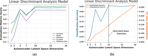
Figure 11. (a) Impact of the autoencoder latent space dimension size on the MLP model’s (a) performance metrics (b) accuracy and computational time.

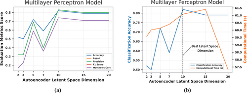
Figure 12. (a) Impact of the autoencoder latent space dimension size on the RF model’s (a) performance metrics (b) accuracy and computational time.

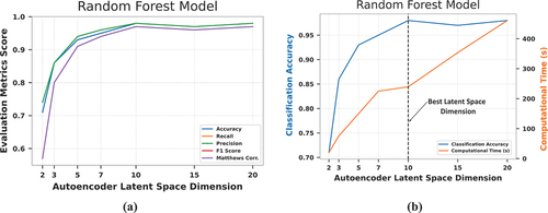
3.2. Effect of the autoencoder latent space dimension on the computational time of the models

Figures 10(b), 11(b), and Figure 12(b) shows the accuracies of the LDA, MLP, and RF models respectively on the left axis, while the right axis of the same figures captures the computational time of the models. From Figure 10(b), a linear positive relationship is observed between the computational time of the LDA model and the AE latent space dimension. A similar relationship is seen between the RF’s computational time and the AE latent space dimension (Figure 12(b)). This linear relationship is intuitive, as the larger the AE’s latent space dimension, the more the number of features to be learned by the ML model which will necessitate a greater investment in computing resources. Within the range of the number of latent space dimensions initially investigated, a non-linear relationship is observed between the MLP’s computation time and the AE latent space dimension, with a peak at 15 (Figure 11(b)). However, further investigations prove that the peak value observed in the graph is only a local maximum. Research over suitably wide dimensional size ranges demonstrates a continual rise in training time for the MLP model with increase in latent space dimension. As depicted in Figures 10(b), 11(b), and Figure 12(b), the optimum AE latent space dimension is 10, as the LDA, MLP, and RF models performed maximally at this dimension while consuming the least amount of computation time.

3.3. Hyperparameter optimization

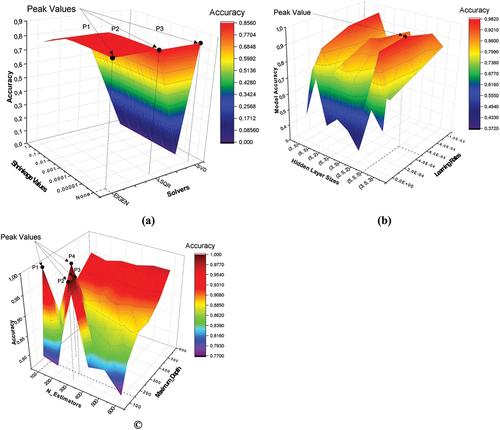
In Section 3.2, the optimal latent space dimension for the AE model was demonstrated to be 10. Consequently, after segmenting the vibration signals into windows of 1000 data samples, the entire dataset was compressed to a feature size of 10 by the AE model and fed to the ML models. The hyperparameters of the LDA, MLP, and RF models were optimized using GA. The best parameters obtained after five generations were collected and used as the reference point for the second phase of hyperparameter tuning. The second phase of hyperparameter tuning was done using the grid-search algorithm. Grid-search was performed using very refined grids around the parameters of the GA. The grid search result for the LDA, MLP and RF model is presented in Figure 13(a–c) and discussed in the subsections that follow.

Figure 13. Hyperparameter optimization plot for (a) the LDA model (b) MLP model (c) RF model.

3.3.1. Linear discriminant analysis model optimization

The LDA model requires an algorithm to compute the log-posterior. Among the estimation algorithms are eigen, LSQR, and SVD. Another important hyperparameter for the LDA model is the shrinkage value, which is a form of regularization used to improve the estimation of covariance matrices. The LDA hyperparameter optimization plot has three peaks, P1, P2 and P3 (Figure 13(a)). At these peaks, the accuracy of the model is 85.4%. At point P1, there is no shrinkage, the estimation algorithm is eigen. At point P2, there is no shrinkage, the estimation algorithm is the LSQR solver. At point P3, there is no shrinkage, the estimation algorithm is SVD. When deciding between the three aforementioned solvers, singular value decomposition is generally recommended because it does not require the computation of covariance matrices and performs well even when the dataset dimension is large [72]. Consequently, point P1, corresponding to a no shrinkage and the SVD estimation algorithm was selected as the final solution to the LDA optimization problem.

3.3.2. Multilayer perceptron model optimization

The most essential hyperparameters of the MLP model are the depth of the MLP, the number of neurons in the hidden layers, the learning rate, and the activation function [72]. The rectified linear unit (ReLU) activation function is generally employed in the hidden layer of the MLP model. ReLU solves the problem of vanishing gradients, enabling the model to coverage to a solution faster [75]. The hyperparameters of the MLP whose values were varied include the learning rate, the depth of the MLP, and the number of neurons in the hidden layers. The hyperparameter optimization plot for the MLP has only one peak (Figure 13(b)). At this peak, the accuracy of the MLP is 98.1%, the learning rate is 0.0005, the model has three hidden layers with five neurons in each layer.

3.3.3. Random forest model optimization

A random forest is an ensemble of decision tree classifiers. It’s essential hyperparameters are the number of trees in the forest (N-Estimators) and the maximum depth of the trees, among others [72]. The hyperparameter optimization plot for the RF model has four peaks, P1-P4 (Figure 13(c)). At these peaks, the accuracy of the model is 100%. The peak at P1, corresponds to 100 decision trees and a maximum depth of 150. The peak at P2, corresponds to 300 decision trees and a maximum depth of 100. The peak at P3 corresponds to 300 decision trees and a maximum depth of 150. The peak at P4 corresponds to 200 decision trees and a maximum depth of 250. When deciding between multiple solutions to a model optimization problem, it is generally recommended to pick the solution that result in the simplest model [76]. On this basis, the solution at peak P1 was selected as the RF’s hyperparameter optimization solution, as the resultant model at this peak has the fewest number of ensemble decision trees.

3.4. Comparison of the performance and computational time of the LDA, MLP and RF after hyperparameter optimization

The performance of the LDA, MLP, and RF models derived from the AE pre-processed vibration signals and optimized with a GA is presented in Table 4 A new nomenclature has been implemented to reflect the new status of the base models. The designations AE-Pre-GO-LDA, AE-Pre-GO-MLP, and AE-Pre-GO-RF denote the genetically optimized AE pre-processed LDA, MLP, and RF models respectively. The AE-Pre-GO-RF model performed best, scoring 100% for classification accuracy and all other performance metrics. The AE-Pre-GO-MLP model came next, with a classification accuracy of 98.1%; similar performance scores were also recorded for other evaluated metrics. The AE-Pre-GO-LDA model had the lowest performance, scoring 85.4% for classification accuracy and similar figures for other evaluated performance parameters. The confusion matrices of the AE-Pre-GO-LDA, AE-Pre-GO-MLP, and AE-Pre-GO-RF are presented in Figure 14(a–c) respectively. The AE-Pre-GO-RF model had no single misclassification. The AE-Pre-GO-MLP had a few misclassifications of the gearbox fault classes. There were more cases of misclassified faults with the LDA-based model compared to its counterparts. Fault 3, 4, 5 and 7 were the most misclassified fault conditions.

Figure 14. (a) Confusion matrix of the AE-Pre-GO-LDA model (b) confusion matrix of the AE-Pre-GO-MLP model (c) confusion matrix of the AE-Pre-GO-RF model (d) comparison of the computation time of the AE-Pre-GO-LDA, AE-Pre-GO-MLP and AE-Pre-GO-RF.

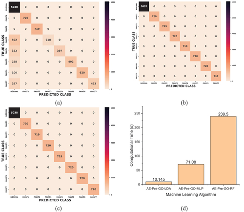
Table 4. Performance of the LDA, MLP and RF models based on the optimized hyperparameters.

Model	Accuracy (%)	Recall or Sensitivity (%)	Precision or Specificity (%)	F1-Score (%)	Matthew’s Correlation (%)	Training Time (s)
AE-Pre-GO-LDA	85.4	85.0	85.6	86.0	80.0	10.14
AE-Pre-GO-MLP	98.1	98.7	97.8	97.7	96.8	71.08
AE-Pre-GO-RF	100.0	100.0	100.0	100.0	100.0	239.50

The exceptional performance of the RF-based model is hardly unexpected. Previous research indicates that numerous authors [77–79] have utilized RF-based models in intelligent fault diagnostics to classify the health status of various types of rotating machinery with a 100% accuracy. This excellent performance of the RF-based model is associated with its ensemble characteristics. Ensemble predictions are derived from multiple ML models, achieving greater efficiency than a single ML model [80]. Moreover, by incorporating random division on subsets of features, the model decorrelates its constituent decision trees, thereby enhancing the accuracy of its predictions [80]. However, as presented in Figure 14(d) and Table 4, the computation time of RF-based model was high compared to the other models. The AE-Pre-GO-MLP model and the AE-Pre-GO-LDA model came next in computational cost. The high computational time in the RF-based model is due to the fact that the prediction time in a RF ensemble is the aggregate of the prediction times of the individual trees in the forest [81].

To ensure a well-informed conclusion, it is imperative to compare the findings of this study with those of similar wind turbine gearbox condition monitoring studies. Table 5 presents the findings of a review of select WT condition monitoring studies that used conventional methods for pre-processing gearbox vibrations. In these studies, vibration processing was performed in two stages: first, feature extraction was performed, and then feature selection or dimensionality reduction was performed. The highest classification accuracy achieved by the models in the studies is presented in the last column. Based on these results, it is seen that the models in our study have comparable classification accuracies with those in conventional studies. But more importantly, whereas the pre-processing of vibration signals in conventional studies requires two phases and expensive feature engineering, our AE-pre-processed models only require a single pre-processing step without feature extraction. Through manifold learning, this study demonstrates how AEs can be employed to mine essential features from raw gearbox vibration signals while simultaneously compressing the data, obviating the need for costly feature engineering.

Table 5. Comparison of wind turbine studies employing conventional methods for pre-processing gearbox vibration signals.

	Vibration Pre-processing Strategies
Reference	Features extraction strategy	Feature reduction technique	Machine learning algorithms	Classification accuracy (%)
[82]	Statistical feature extraction after empirical model decomposition	Decision tree feature selection	Support vector machine (SVM)	92.80
[83]	Time domain statistical feature extraction	Dynamic principal component analysis (DPCA)	Support vector machine (SVM)	82.0
[84]	Discrete wavelet transform followed by extraction of statistical features	Sequential feature selection	Artificial neural network (ANN) and support vector machine (SVM)	100.0
[85]	Histogram feature extraction	Feature selection using J48 decision tree algorithm.	K-nearest neighbour (KNN)	93.8
[27]	Time domain statistical feature extraction after empirical mode decomposition with adaptive noise. Frequency domain feature extraction after fast Fourier transform (FFT)	Recursive feature elimination (RFE) combined with chi-square test	Extreme learning machine (ELM) and support vector machine (SVM)	99.6
[86]	Feature extraction after discrete wavelet transforms (DWT)	Dimensionality reduction using singular value decomposition	Extreme learning machine (ELM)	99.9
This study	Manifold learning with AE		AE-Pre-GO-LDA	80
This study	Manifold learning with AE		AE-Pre-GO-MLP	96
This study	Manifold learning with AE		AE-Pre-GO-RF	100

4. Conclusion and future perspectives

4.1. Conclusion

The current investigation aimed to develop a novel AE pre-processing framework for vibration-based fault diagnosis in a WT gearbox. Windowed vibration signals are fed to fully connected AE layers to automatically learn the features in the vibration data while compressing the data, obviating the need for costly feature engineering and dimensionality reduction. The compressed features are fed to select downstream classifiers to identify the gearbox fault categories. The impact of the size of the AE’s latent space on the quality of features extracted, as evidenced by the classification performance of the downstream ML models, is investigated. Further, the study investigates the impact of the size of the AE’s latent space on the computational time of the downstream machine-learning models. The final AE model is designed based on the optimal latent space dimension. Three ML models, including LDA, MLP, and RF, are trained with the compressed representation of the vibration signals extracted from the AE’s latent space. The hyperparameters of the downstream classifiers are optimized by GA. The proposed methodologies are validated by experimental data sourced from the NREL’s Vibration Condition Monitoring Benchmarking Datasets. As a contribution to the wind turbine literature, the study’s findings provide an alternate technique to dealing with high-dimensional vibration data that avoids the time-consuming feature extraction process while producing accurate results. The important findings of the study are summarized as follows:

1. For accurate fault diagnosis, the optimal latent space dimension must be chosen for AE models employed in pre-processing vibration signals for wind turbine fault diagnostic models. The results of the current investigation demonstrate that the performance of the downstream models depends on the size of the AE’s latent space. As the size of the AE’s latent space increased, the quality of features extracted improved until a plateau was observed at a latent space dimension of 10.

2. The computational time of the downstream classifiers had a linear positive relationship with the size of the AE’s latent space. This means that as the latent space increases the computational resources required for the model development increases.

3. The RF model trained for the longest period of time, followed by the MLP and the LDA models. The AE-Pre-GO-RF model had the highest classification accuracy (100%), then the AE-Pre-GO-MLP (98.1%) and the AE-Pre-GO-LDA model (85.4%). The AE-Pre-GO-RF model is thus recommended for accurate condition monitoring of the wind turbine gearbox.

4. Both sensitivity and specificity for all the developed models were high. Therefore, implementing the proposed models for wind turbine condition monitoring will minimize the incidence of turbine false alarms.

5. The findings of the study demonstrate that the proposed AE vibration pre-processing framework is effective for multi-defect identification in WT gearboxes.

4.2. Future perspectives

This study proposed an AE pre-processing framework for diagnosing faults in a wind turbine gearbox using vibration data. Future research could examine the generalizability of this technique by employing the proposed methodology on other rotating components of WTs, such as the generator bearing and the main shaft bearing [87]. In addition, while the current investigation applied the proposed framework to turbine condition monitoring vibration data, future research could investigate the application of the same framework to turbine SCADA, where the curse of dimensionality is also a challenge.

Abbreviations

AE	=	Autoencoder
AE-Pre-GO-	=	Autoencoder pre-processed genetically optimized-
CWT	=	Continuous wavelet transforms
DWT	=	Discrete wavelet transforms
EMD	=	Empirical mode decomposition
FE-DR	=	Feature extraction – dimensionality reduction
FE-FS	=	Feature extraction – feature selection
FN	=	False negative
FP	=	False positive
GA	=	Genetic algorithm
KPCA	=	Kernel principal component analysis
LDA	=	Linear discriminant analysis
LSQR	=	least-squares
MAE	=	Mean absolute error
MCC	=	Matthew’s correlation coefficient
ML	=	Machine learning
MLP	=	Multilayer perceptron
NREL	=	National renewable energy laboratory
PCA	=	Principal component analysis
ReLU	=	Rectified Linear Unit
RF	=	Random forest
SCADA	=	Supervisory control and data acquisition
STFT	=	Short-time Fourier transform
SVD	=	Single-value decomposition
TN	=	True negative
TP	=	True positive
t-SNE	=	t-Distributed stochastic neighbor embedding
VMD	=	Variational mode decomposition
WT	=	Wind turbine

Nomenclature

b	=	Bias vector
CE	=	Cross entropy
F1-score	=	Harmonic mean of precision and recall
$\mathit{H}()$	=	Loss function
j	=	Data feature
$J_{\mathit{AE}}$	=	Autoencoder optimization operator
L1	=	Norm loss
N-Estimators	=	Number of estimators (decision trees)
Qm	=	Data at node m
${\mathrm{S}}_b$	=	Between-class scatter matrix
${\mathrm{S}}_w$	=	Within-class scatter matrix
s	=	Seconds
tm	=	Decision tree split threshold
tr(.)	=	Matrix trace operation
W	=	Weight matrix
$x_i$	=	Actual input
${\hat{x}}_{\mathit{i}}$	=	Reconstructed input
$y_i$	=	Ground truth
${\hat{y}}_{\mathit{i}}$	=	Predicted output
z	=	Autoencoder latent space representation
φ	=	Activation function
(.)T	=	Matrix transpose operation
$\mathit{\theta }$	=	Decision tree split operation

CRediT authorship contribution statement

Samuel M. Gbashi: Writing – original draft, Writing – review and editing, Visualization, Modelling, Data curation; Obafemi O. Olatunji: Supervision, Conceptualization, Methodology, Writing – review and editing. Paul A. Adedeji: Supervision, Data curation, Conceptualization, Methodology, Writing – review and editing. Nkosinathi Madushele: Funding, Supervision, Conceptualization, Methodology.

Disclosure statement

The authors affirm that they have no known competing financial interests or ties to other parties that may have potentially influenced the findings presented in this study.

Additional information

Funding

The authors acknowledge the financial support from the University of Johannesburg and the National Research Foundation through the Thuthuka Grant [129742] and the Department of Energy/National Renewable Energy Laboratory for providing the data for the study.

References

- Gbashi SM, Adedeji PA. Hyperparameter optimization on CNN using hyperband for fault identification in wind turbine high-speed shaft gearbox bearing. 2023 November;16–17.
- Alotaibi M, Honarvar Shakibaei Asli B, Khan M. Non-invasive inspections: a review on methods and tools. Sensors. 2021;21(24):8474. doi:10.3390/s21248474
- Ogaili AAF, Hamzah MN, Jaber AA. Enhanced fault detection of wind turbine using extreme gradient boosting technique based on nonstationary vibration analysis. J Fail Anal And Preven. 2024;24(2):877–895. doi: 10.1007/s11668-024-01894-x
- Ogaili AA, Hamzah MN, Jaber AA, et al. Application of discrete wavelet transform for condition monitoring and fault detection in wind turbine blades: an experimental study. Eng Techol J. 2024;42(1):104–116. doi: 10.30684/etj.2023.142023.1516
- Li X, Wang Y, Yao J, et al. Multi-sensor fusion fault diagnosis method of wind turbine bearing based on adaptive convergent viewable neural networks. Reliab Eng Syst Saf. 2024;245:109980. doi: 10.1016/j.ress.2024.109980
- Narasinh V, Mital P, Chakravortty N, et al. Investigating power loss in a wind turbine using real-time vibration signature. Eng Fail Anal. 2024;159:108010. doi: 10.1016/j.engfailanal.2024.108010
- Brethee KF, Ibrahim GR, Albarbar A-H, et al. Vibro-acoustic analysis for remotely condition monitoring approach of wind turbine. AIP Conf Proc. 2024;3009(1):030036.
- Jaber AA. Diagnosis of bearing faults using temporal vibration signals: a comparative study of machine learning models with feature selection techniques. J Fail Anal And Preven. 2024;24(2):752–768. doi: 10.1007/s11668-024-01883-0
- Wang J, Fu P, Zhang L, et al. Multilevel information fusion for induction motor fault diagnosis. IEEE/ASME Trans Mechatron. 2019;24(5):2139–2150. doi:10.1109/TMECH.2019.2928967
- Alharbi F, Luo S, Zhang H, et al. A brief review of acoustic and vibration signal-based fault detection for belt conveyor idlers using machine learning models. Sensors. 2023;23(4):1902. doi: 10.3390/s23041902
- Daiki G, Tsuyoshi I, Takekiyo H, et al. Failure diagnosis and physical interpretation of journal bearing for slurry liquid using long-term real vibration data. Struct Heal Monit. 2024;23(2):1201–1216. doi: 10.1177/14759217231184579
- Tang H, Tang Y, Su Y, et al. Feature extraction of multi-sensors for early bearing fault diagnosis using deep learning based on minimum unscented Kalman filter. Eng Appl Artif Intell. 2024;127:107138. doi: 10.1016/j.engappai.2023.107138
- Nayana BR, Geethanjali P. Analysis of statistical time-domain features effectiveness in identification of bearing faults from vibration signal. IEEE Sens J. 2017;17(17):5618–5625. doi:10.1109/JSEN.2017.2727638
- Pang B, Liu Q, Sun Z, et al. Time-frequency supervised contrastive learning via pseudo-labeling: an unsupervised domain adaptation network for rolling bearing fault diagnosis under time-varying speeds. Adv Eng Informatics. 2024;59:102304. doi: 10.1016/j.aei.2023.102304
- Li H, Wang D. Multilevel feature fusion of multi-domain vibration signals for bearing fault diagnosis. Signal Image Video Process. 2024;18(1):99–108. doi: 10.1007/s11760-023-02715-8
- Buchaiah S, Shakya P. Bearing fault diagnosis and prognosis using data fusion based feature extraction and feature selection. Measurement. 2022;188:110506. doi:10.1016/j.measurement.2021.110506
- Song Y, Cao J, Hu Y. In-process feature extraction of milling chatter based on second-order synchroextracting transform and fast kutrogram. Mech Syst Signal Process. 2024;208:111018. doi:10.1016/j.ymssp.2023.111018
- Li H, Zhang J, Zhang Z, et al. Priori-distribution-guided adaptive sparse attention for cross-domain feature mining in diesel engine fault diagnosis. Eng Appl Artif Intell. 2024;132:107975. doi: 10.1016/j.engappai.2024.107975
- Elias S. Vibration improvement of offshore wind turbines under multiple hazards. Structures. 2024;59:105800. doi: 10.1016/j.istruc.2023.105800
- Javorskyj I, Yuzefovych R, Lychak O, et al. Hilbert transform for covariance analysis of periodically nonstationary random signals with high-frequency modulation. ISA Trans. 2024;144:452–481. doi:10.1016/j.isatra.2023.10.025
- Gbashi SM, Olatunji OO, Adedeji PA, et al. A hybrid empirical mode decomposition (EMD)-support vector machine (SVM) for multi-fault recognition in a wind turbine gearbox. 2023 International Conference on Electrical, Computer and Energy Technologies (ICECET); 2023. p. 1–7. doi: 10.1109/ICECET58911.2023.10389608
- Akan A, Cura OK. Time–frequency signal processing: today and future. Digit Signal Process. 2021;119:103216. doi: 10.1016/j.dsp.2021.103216
- Vashishtha G, Kumar R. Pelton wheel bucket fault diagnosis using improved Shannon entropy and expectation maximization principal component analysis. J Vib Eng Technol. 2022;10(1):335–349. doi: 10.1007/s42417-021-00379-7
- Chauhan S, Vashishtha G, Kumar R, et al. An adaptive feature mode decomposition based on a novel health indicator for bearing fault diagnosis. Measurement. 2024;226:114191. doi: 10.1016/j.measurement.2024.114191
- Vashishtha G, Chauhan S, Singh M, et al. Bearing defect identification by swarm decomposition considering permutation entropy measure and opposition-based slime mould algorithm. Measurement. 2021;178:109389. doi:10.1016/j.measurement.2021.109389
- Vashishtha G, Chauhan S, Yadav N, et al. A two-level adaptive chirp mode decomposition and tangent entropy in estimation of single-valued neutrosophic cross-entropy for detecting impeller defects in centrifugal pump. Appl Acoust. 2022;197:108905. doi:10.1016/j.apacoust.2022.108905
- Tang Z, Wang M, Ouyang T, et al. A wind turbine bearing fault diagnosis method based on fused depth features in time–frequency domain. Energy Rep. 2022;8:12727–12739. doi:10.1016/j.egyr.2022.09.113
- Wang T, Han Q, Chu F, et al. Vibration based condition monitoring and fault diagnosis of wind turbine planetary gearbox: a review. Mech Syst Signal Process. 2019;126:662–685. doi:10.1016/j.ymssp.2019.02.051
- Hasan MJ, Sohaib M, Kim J-M. An explainable ai-based fault diagnosis model for bearings. Sensors. 2021;21(12):4070. doi:10.3390/s21124070
- Jović A, Brkić K, Bogunović N. A review of feature selection methods with applications. 2015 38th Int Convention On Inf And Commun Technol, Electron And Microelectronics (MIPRO). 2015;1(1): 1200–1205.
- Žvokelj M, Zupan S, Prebil I. Non-linear multivariate and multiscale monitoring and signal denoising strategy using kernel principal component analysis combined with ensemble empirical mode decomposition method. Mech Syst Signal Process. 2011;25(7):2631–2653. doi:10.1016/j.ymssp.2011.03.002
- Mordohai P, Medioni G,” S. Z. Li and A. Jain, editors. Manifold learning BT – Encyclopedia of Biometrics. Boston (MA): Springer US; 2009. p. 954–958. doi: 10.1007/978-0-387-73003-5_301
- Duque AF, Morin S, Wolf G, et al. Extendable and invertible manifold learning with geometry regularized autoencoders. 2020 IEEE International Conference on Big Data (Big Data); Atlanta, GA, USA. 2020. p. 5027–5036.
- Jordan J. Introduction to autoencoders. Datascience. 2018. Available from: https://www.jeremyjordan.me/autoencoders/
- González-Muñiz A, Díaz I, Cuadrado AA, et al. Two-step residual-error based approach for anomaly detection in engineering systems using variational autoencoders. Comput Electr Eng. 2022;101:108065. doi:10.1016/j.compeleceng.2022.108065
- Nam K, Wang F. An extreme rainfall-induced landslide susceptibility assessment using autoencoder combined with random forest in Shimane Prefecture, Japan. Geoenvironmental Disasters. 2020;7(1):1–16. doi: 10.1186/s40677-020-0143-7
- Zhang C, Hu D, Yang T. Anomaly detection and diagnosis for wind turbines using long short-term memory-based stacked denoising autoencoders and XGBoost. Reliab Eng Syst Saf. 2022;222:108445. doi:10.1016/j.ress.2022.108445
- Chopra P, Yadav SK. Fault detection and classification by unsupervised feature extraction and dimensionality reduction. Complex Intell Syst. 2015;1(1–4):25–33. doi: 10.1007/s40747-015-0004-2
- Mishra KM, Krogerus TR, Huhtala KJ. Fault detection of elevator systems using deep autoencoder feature extraction. 2019 13th International Conference on Research Challenges in Information Science (RCIS); Brussels, Belgium. 2019. p. 1–6.
- Venkatesh B, Anuradha J. A review of feature selection and its methods. Cybern Inf Technol. 2019;19(1):3–26. doi: 10.2478/cait-2019-0001
- Wu H, Chen J, Liu X, et al. One-dimensional CNN-based intelligent recognition of vibrations in pipeline monitoring with DAS. J Light Technol. 2019;37(17):4359–4366. doi: 10.1109/JLT.2019.2923839
- Sahu B, Dash S. Optimal feature selection from high-dimensional microarray dataset employing hybrid IG-Jaya model. Curr Mater Sci Former Recent Patents Mater Sci. 2024;17(1):21–43. doi: 10.2174/2666145416666230124143912
- Fan Y, Liu J, Tang J, et al. Learning correlation information for multi-label feature selection. Pattern Recognit. 2024;145:109899. doi: 10.1016/j.patcog.2023.109899
- Mostafa RR, Khedr AM, Al Aghbari Z, et al. An adaptive hybrid mutated differential evolution feature selection method for low and high-dimensional medical datasets. Knowledge-Based Syst. 2024;283:111218. doi: 10.1016/j.knosys.2023.111218
- Rao S, Zou G, Yang S, et al. A feature selection and ensemble learning based methodology for transformer fault diagnosis. Appl Soft Comput. 2024;150:111072. doi:10.1016/j.asoc.2023.111072
- Dai J, Huang W, Zhang C, et al. Multi-label feature selection by strongly relevant label gain and label mutual aid. Pattern Recognit. 2024;145:109945. doi: 10.1016/j.patcog.2023.109945
- Wang Y, Ran S, Wang G-G. Role-oriented binary grey wolf optimizer using foraging-following and lévy flight for feature selection. Appl Math Model. 2024;126:310–326. doi:10.1016/j.apm.2023.08.043
- Sarita K, Devarapalli R, Kumar S, et al. Principal component analysis technique for early fault detection. J Intell Fuzzy Syst. 2022;42(2):861–872. doi:10.3233/JIFS-189755
- Pozo F, and Vidal Y. Damage and Fault Detection of Structures Using Principal Component Analysis and Hypothesis Testing. In: Naik GR, editor. Advances in Principal Component Analysis. Singapore: Springer; 2018. p. 137–191. doi: 10.1007/978-981-10-6704-4_7
- Wang Z, Zhang G, Xing X, et al. Comparison of dimensionality reduction techniques for multi-variable spatiotemporal flow fields. Ocean Eng. 2024;291:116421. doi: 10.1016/j.oceaneng.2023.116421
- Liu L, Liu J, Wang H, et al. A multivariate monitoring method based on kernel principal component analysis and dual control chart. J Process Control. 2023;127:102994. doi: 10.1016/j.jprocont.2023.102994
- Yang Z, Xu B, Luo W, et al. Autoencoder-based representation learning and its application in intelligent fault diagnosis: a review. Measurement. 2022;189:110460. doi:10.1016/j.measurement.2021.110460
- Sarkodie K, Fergusson-Rees A, Abdulkadir M, et al. Gas-liquid flow regime identification via a non-intrusive optical sensor combined with polynomial regression and linear discriminant analysis. Ann Nucl Energy. 2023;180:109424. doi:10.1016/j.anucene.2022.109424
- Zhang R, Xu P, Guo L, et al. Z-score linear discriminant analysis for EEG based brain-computer interfaces. PLoS One. 2013;8(9):e74433. doi:10.1371/journal.pone.0074433
- Singh G, Pal Y, Dahiya AK. Classification of power quality disturbances using linear discriminant analysis. Appl Soft Comput. 2023;138:110181. doi: 10.1016/j.asoc.2023.110181
- Lipshutz D, Kashalikar A, Farashahi S, et al. A linear discriminant analysis model of imbalanced associative learning in the mushroom body compartment. PLoS Comput Biol. 2023;19(2):e1010864. doi:10.1371/journal.pcbi.1010864
- Dragović S. Artificial neural network modeling in environmental radioactivity studies – A review. Sci Total Environ. 2022;847:157526. doi: 10.1016/j.scitotenv.2022.157526
- Juan NP, Valdecantos VN. Review of the application of artificial neural networks in ocean engineering. Ocean Eng. 2022;259:111947. doi:10.1016/j.oceaneng.2022.111947
- Al Barsh YI, Duhair MK, Ismail HJ, et al. MPG prediction using artificial neural network. Int J Acad Inf Syst Res. 2020;4(11):7–16.
- Oliveira TP, Barbar JS, Soares AS. Computer network traffic prediction: a comparison between traditional and deep learning neural networks. Int J Big Data Intell. 2016;3(1):28–37. doi: 10.1504/IJBDI.2016.073903
- Ibrahim MH, Jihad KH, Kamal LL. Determining optimum structure for artificial neural network and comparison between back-propagation and Levenberg-Marquardt training algorithms. Int J Eng Sci. 2017;14887:14887–14890.
- Sun Z, Wang G, Li P, et al. An improved random forest based on the classification accuracy and correlation measurement of decision trees. Expert Syst Appl. 2024;237:121549. doi:10.1016/j.eswa.2023.121549
- Irsoy O, Alpaydın E. Distributed decision trees. Proceedings, Structural, Syntactic, and Statistical Pattern Recognition: Joint IAPR International Workshops, S+ SSPR 2022; Montreal, QC, Canada; 2023. p. 152–162. [2022 Aug 26–27].
- Zheng J, Liu Y, Ge Z. Dynamic ensemble selection based improved random forests for fault classification in industrial processes. IFAC J Syst Control. 2022;20:100189. doi: 10.1016/j.ifacsc.2022.100189
- Hu Q, Si X-S, Zhang Q-H, et al. A rotating machinery fault diagnosis method based on multi-scale dimensionless indicators and random forests. Mech Syst Signal Process. 2020;139:106609. doi:10.1016/j.ymssp.2019.106609
- Chauhan S, Vashishtha G. A synergy of an evolutionary algorithm with slime mould algorithm through series and parallel construction for improving global optimization and conventional design problem. Eng Appl Artif Intell. 2023;118:105650. doi:10.1016/j.engappai.2022.105650
- Adedeji PA, Olatunji OO, Madushele N, et al. Evolutionary-based hyperparameter tuning in machine learning models for condition monitoring in wind turbines–a survey. 2021 IEEE 12th International Conference on Mechanical and Intelligent Manufacturing Technologies (ICMIMT); Cape Town, South Africa. 2021. p. 254–258.
- Olatunji OO, Adedeji PA, Madushele N, et al. Evolutionary optimization of biogas production from food, fruit, and vegetable (FFV) waste. Biomass Convers Biorefinery. 2023:1–13. doi: 10.1007/s13399-023-04506-0
- Hollweg GV, de Oliveira Evald PJD, Mattos E, et al. Self-tuning methodology for adaptive controllers based on genetic algorithms applied for grid-tied power converters. Control Eng Pract. 2023;135:105500. doi: 10.1016/j.conengprac.2023.105500
- Adeleke O, Akinlabi S, Jen T-C, et al. Evolutionary-based neuro-fuzzy modelling of combustion enthalpy of municipal solid waste. Neural Comput Appl. 2022;34(10):7419–7436. doi:10.1007/s00521-021-06870-2
- Katoch S, Chauhan SS, Kumar V. A review on genetic algorithm: past, present, and future. Multimed Tools Appl. 2021;80(5):8091–8126. doi: 10.1007/s11042-020-10139-6
- Pedregosa F,Varoquaux, G., Gramfort, A et al. Scikit-learn: machine learning in python. J Mach Learn Res. 2011;12:2825–2830.
- Shao G, Tang L, Zhang H. Introducing image classification efficacies. IEEE Access. 2021;9:134809–134816. doi:10.1109/ACCESS.2021.3116526
- Trunz E, Weinmann M, Merzbach S, et al. Efficient structuring of the latent space for controllable data reconstruction and compression. Graph Vis Comput. 2022;7:200059. doi: 10.1016/j.gvc.2022.200059
- Ide H, Kurita T. Improvement of learning for CNN with ReLU activation by sparse regularization. 2017 international joint conference on neural networks (IJCNN); Anchorage, AK, USA. 2017. p. 2684–2691.
- Guan S, Loew M. Analysis of generalizability of deep neural networks based on the complexity of decision boundary. 2020 19th IEEE International Conference on Machine Learning and Applications (ICMLA); Miami, FL, USA. 2020. p. 101–106.
- Okumus H, Nuroglu FM. A random forest-based approach for fault location detection in distribution systems. Electr Eng. 2021;103(1):257–264. doi: 10.1007/s00202-020-01074-8
- Sun Y, Zhang H, Zhao T, et al. A new convolutional neural network with random forest method for hydrogen sensor fault diagnosis. IEEE Access. 2020;8:85421–85430. doi:10.1109/ACCESS.2020.2992231
- Tang X, Gu X, Rao L, et al. A single fault detection method of gearbox based on random forest hybrid classifier and improved Dempster-Shafer information fusion. Comput Electr Eng. 2021;92:107101. doi: 10.1016/j.compeleceng.2021.107101
- Sagi O, Rokach L. Ensemble learning: a survey. Wiley Interdiscip Rev Data Min Knowl Discov. 2018;8(4):e1249. doi: 10.1002/widm.1249
- Xu G, Liu M, Jiang Z, et al. Bearing fault diagnosis method based on deep convolutional neural network and random forest ensemble learning. Sensors. 2019;19(5):1088. doi:10.3390/s19051088
- Inturi V, Sabareesh GR, Sharma V. Integrated vibro-acoustic analysis and empirical mode decomposition for fault diagnosis of gears in a wind turbine. Procedia Struct Integr. 2019;14(2018):937–944. doi: 10.1016/j.prostr.2019.07.074
- Kordestani M, Rezamand M, Orchard M, et al. Planetary gear faults detection in wind turbine gearbox based on a ten years historical data from three wind farms. IFAC-Papersonline. 2020;53(2):10318–10323. doi: 10.1016/j.ifacol.2020.12.2767
- Biswal S, George JD, Sabareesh GR. Fault size estimation using vibration signatures in a wind turbine test-rig. Procedia Eng. 2016;144:305–311. doi:10.1016/j.proeng.2016.05.137
- Joshuva A, Sugumaran V. A lazy learning approach for condition monitoring of wind turbine blade using vibration signals and histogram features. Measurement. 2020;152:107295. doi:10.1016/j.measurement.2019.107295
- Pang Y, Jia L, Zhang X, et al. Design and implementation of automatic fault diagnosis system for wind turbine. Comput Electr Eng. 2020;87:106754. doi: 10.1016/j.compeleceng.2020.106754
- Gbashi SM, Madushele N, Olatunji OO, et al. Wind turbine main bearing: a mini review of its failure modes and condition monitoring techniques. 2022 IEEE 13th International Conference on Mechanical and Intelligent Manufacturing Technologies (ICMIMT); 25-27 May 2022; Cape Town, South Africa. 2022. doi: 10.1109/ICMIMT55556.2022.9845317