Mechanism of high-speed train carbody shaking due to degradation of wheel-rail contact geometry

ABSTRACT

The carbody shaking phenomenon (CSP) can greatly reduce the ride comfort of high-speed trains. To investigate the abnormal vibration feature and causes of the CSP, extensive field measurements and numerical simulations were conducted. A three-dimensional rigid-flexible coupled dynamic model of a high-speed vehicle is constructed to reproduce the CSP and reveal the key influence factors, in which the finite element model of the carbody is updated based on the experimental modal data. The field test show that the main vibration frequency of the carbody accelerations appear around 7.90 Hz, which is close to the natural frequency of the carbody diamond mode. The simulation results demonstrate that the CSP is caused by the carbody resonance vibrations induced by bogie hunting motion, which is triggered by the deterioration of wheel-rail contact geometry. When the train passes through turnouts at high speed, wheel-rail impact will further aggravate the CSPs. 

KEYWORDS:

• High-speed train
• carbody shaking phenomenon
• flexible resonance
• hunting motion
• wheel-rail contact
• degradation

1. Introduction

High-speed trains are widely used in China for people to travel medium and long distances due to the high ride comfort and convenience. Owing to the complex operation environment, high travel speed, lightweight design of carbody, degradation of wheel-rail matching and significant increase in departure frequency, etc., more and more faults related to the HST ride stability and comfort appear [1,2]. It not only poses a negative effect on ride comfort but also may threaten railway safety, leading to serious problems, such as fatigue damage of HST components. For example, a new type of Chinese HST has maintained satisfactory performance since it was put into operation. However, it is reported that the CSP appeared in several vehicles of this type of HST recently when running at a high speed of 350 km/h recently. This abnormal vibration phenomenon mainly occurred near the railway stations, which led to the high-frequency violent shaking of the high-speed train carbody, and the ride comfort was obviously reduced. In order to investigate the causes and countermeasures of the HST CSP, the authors carried out extensive experiments and numerical analyses, which has motivated the present study.

A large number of scholars have made theoretical and field experimental studies on the elastic vibrations of high-speed railway vehicles. Wei [3] and Shi [4] carried out the identification of HST carbody modes based on laboratory tests, and these tests matched with the modes of carbody vibration on site. Li et al. [5] proposed an improved modal superposition approach for fatigue simulation of the carbody under CSP conditions. Qi et al. [6] discovered the relationship between the abnormal vibration of various railway lines and the carbody in a field test and developed a technique to minimize the carbody abnormal vibration by adjusting the stiffness of the anti-yaw damper and the longitudinal positioning stiffness of the wheelset. Morales et al. [7] argued that passengers not only play the function of extra mass in vehicle vibration research, but also the role of dynamic vibration absorbers (DVAs), which may alter the vehicle mode.

In addition, other types of railway vehicles have similar abnormal vibration problems. Yang [8] and Tao [9] identified higher-order wheel polygons as the root cause of the abnormal vibration of locomotives, through tracking tests on more than 40 locomotives. Sun [10] claimed that inadequate wheel-rail contact conicity was the major source of the low-frequency locomotive shaking, and decreasing the stiffness and damping of the anti-yaw damper might suppress carbody abnormal vibrations. By establishing a theoretical model with 17 degrees of freedom (DOFs), it was verified in the studies of Xia et al. and Gong et al. [11,12] that the abnormal change of modal damping of the vehicle system was the root of the abnormal vibration of the vehicle. At the same time, the researchers put forward solutions to deal with vehicle abnormal vibration from the perspectives of optimizing the position or hanging parameters of the equipment under the carbody underframe, installing the DVA for the bogie, and optimizing the design of the bogie suspension system [13–18].

According to current research on vehicle abnormal vibration, the degradation of wheel-rail contact, failure of vehicle suspension mechanisms and deterioration of track structure may all cause the abnormal vibration of train carbody, and wheel-rail matching is the fundamental reason [19,20]. When the frequency of bogie hunting motion approaches the natural modal frequency of the vehicle system, resonance will occur, especially when the vehicle passes through specific railway sections. The most typical symptoms are low-frequency sway of the carbody and high-frequency shaking of the carbody. However, the core reason of HST carbody shaking problem is still unclear. At present, the simulation research of CSP is still relatively lacking. Particularly in terms of the systematic compilation of knowledge on the causes and vibration characteristics of CSP at the mechanism level.

The objective of this paper is to explore the mechanism of the HST CSP from the perspective of vehicle-track coupled model and rigid-flexible coupled dynamics theory and simulate and reproduce the elastic deformation of carbody on site. The rest content of this paper is outlined as follows: Section 2 introduces the field test of the HST CSP and will give typical vibration characteristics of the CSP and its influence on ride comfort. Section 3 presents the FE model updating of carbody (the basis for modelling coupled vehicle-track dynamics and accurate simulation reproduction of CSP). The FE and MBS coupling (FE-MBS) method was utilized to establish a rigid-flexible coupled model. Section 4 shows the dynamic simulations and analysis of the mechanism of the HST CSP, from the standpoint of wheel-rail profile matching and vehicle passing through the railway station turnouts at high speed. Section 5 presents the findings and recommendations for further study. As there are many abbreviations in this paper, the full name and specific meaning are given in the abbreviations list.

Table

Abbreviation
CSP	Carbody shaking phenomenon
HST	High-speed train
DM	Diamond mode
FEM	Finite element method
DAQ	Data acquisition system
GPS	Global positioning system
CWT	Continuous wavelet transform
WWP	Worn wheel profile
SWP	Standard wheel profile
BGRP	Before grinding rail profile
AGRP	After grinding rail profile
SRP	Standard rail profile
MAC	Modal assurance criterion
CBMSM	Craig-Bampton modal synthesis method
MBD	Multibody dynamics

2. Experimental investigation on abnormal vibration caused by CSP

2.1. Field test

Recently, CSPs appeared on the trailers of several high-speed trains with a maximum running speed of 350 km/h. The passengers felt extremely uncomfortable due to the abnormal vibration, which has attracted the attention of railway authorities. Therefore, the authors carried out a specific experiment on CSP. As illustrated in Figure 1(a–c), the on-board data acquisition system (DAQ) was utilized to continually record accelerations using accelerometers positioned on the bogie frame above the wheelset, as well as the front and rear floor of the carbody. The former is used to determine the operation stability of the vehicle, while the latter is used to evaluate the ride comfort of the carriage. The global positioning system (GPS) device mainly records information such as the speed and position of the vehicle, which is convenient for judging the section and speed where CSP appears.

Figure 1. Field test: (a) Measuring points arrangement; (b) Accelerometer on axle box above wheelset; (c) Accelerometers on carbody floor; (d) DAQ equipment.

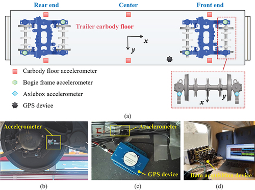
Six measure points were put on the floor to make it easier to compare the vibration characteristics at various places of the carbody floor. The lateral distance between the two measuring points is 2 m. Meanwhile, we employed the profile-measuring tool to record the wheel profiles in worn condition, which will be discussed later in detail. The core equipment of DAQ testing system is the HBM SoMat eDAQ data collector, as shown in Figure 1(d). All of the sensors employed in the experiments were three-dimensional sensors with a signal sampling rate of 4096 Hz. The operating mileage of the tested HST after wheel re-profile was about 224,000 km. During the test, the train operated without passengers on a no-load basis. The test area was the Beijing-Shanghai high-speed railway located between Shanghai and Nanjing in eastern China.

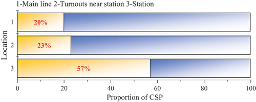
The distribution of CSP positions acquired by the GPS device is shown in Figure 2. The CSPs mainly occurred along sections of the railway main line, at railway stations, and 1 km around stations, with stations being the most prone to shaking, accounting for over 80% of the CSPs. Railway station area happens to be the area where turnouts are relatively concentrated, and there are many switch turnouts. The passing speed of the train at this moment was between 345 km/h and 350 km/h.

Figure 2. Statistics of CSPs location.

2.2. Experimental results

2.2.1. Ride comfort evaluation

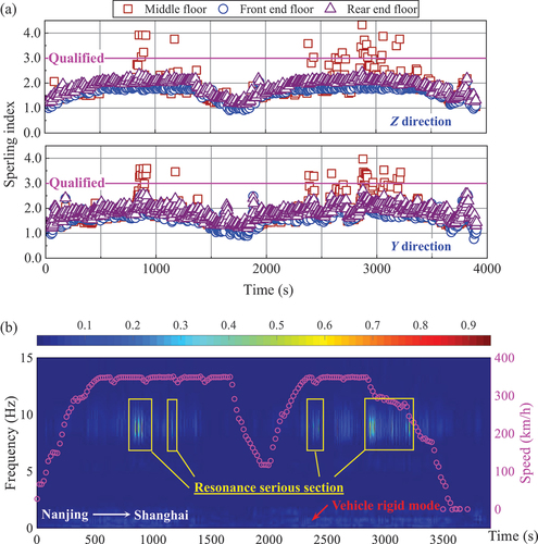
Figure 3(a) shows the ride comfort index (Sperling index) for the front, middle, and rear floor locations of the carbody for the whole operation period. According to China’s high-speed train dynamics code GB 5599–2019, when the Sperling index W_S is greater than 3, it will be regarded as unqualified. For the good, medium, and qualified grades, the maximum values of the Sperling index are 2.5, 2.75, and 3.0, respectively. In Figure 3(b), the middle floor measurement points were selected for time-frequency analysis, and the Morlet continuous wavelet transform (CWT) analysis method was performed to extract time-frequency features of the CSPs. It has the characteristics of multiresolution analysis and can characterize the local characteristics of signals in time domain and frequency domain. The discrete data points in magenta in the figure represent the speed information recorded by GPS. From Figure 3, the following information was obtained:

1. The uncomfortable phenomenon generated by the CSP was concentrated during the running speed was approximately 350 km/h, when the vertical and lateral W_S reached maximum values of 4.31 and 4.02, respectively. Therefore, the CSP has a great negative impact on the ride comfort of passengers.

2. The vertical exceedance of the floor was more serious than the lateral exceedance, and the central floor was worse than the front and rear floor. The duration of CSP varies from several seconds to tens of seconds, depending on the state of the railway line.

3. The time-frequency diagram monitors the frequency bands of 8 Hz and 0.5–2 Hz during operation. When this indication is exceeded, the energy at 8 Hz rises sharply, and the colour on the CWT becomes darker. The vertical sensitive frequency of human body is just 4–8 Hz. So at this time, the passengers will obviously feel distressed.

Figure 3. (a) Sperling index of front, middle and rear position of floor; (b) CWT of vertical acceleration in middle floor.

To prevent phase delay induced by filtering, the acceleration signals are processed by a fourth-order Butterworth filter with a cut-off frequency of 0.3 to 15 Hz [5]. The vertical accelerations of the two measurement points on the middle floor are within 0.05 g of the vehicle in the normal section. But when the carbody shaking condition occurs, the acceleration fluctuates around 0.15 g, with a three-fold overall expansion, and the CSP lasts for about 20 s, as shown in Figure 4(a). The acceleration reaches the maximum value of 0.172 g. In Figure 4(c), the diagonal measurement points of bogie frame were selected for research, and the peak value reaches 0.771 g. Due to the guiding effect of the front wheelset, the front end of the frame vibrates more intensively. When CSP develops, both the carbody and the frame show significant harmonic vibration (see Figure 4(b,d)).

Figure 4. Test results for the vehicle: (a) Vertical acceleration of middle floor; (b) Partial enlargement of Figure (a); (c) Lateral acceleration of bogie frame; (d) Partial enlargement of Figure (c); (e) PSD comparison of middle floor, frame and axle box; (f) Identified carbody DM in modal testing.

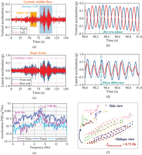
As shown in Figure 4(e), it is obvious that in the Power Spectral Density (PSD) curves, the carbody floor, bogie frame, and axle box have significant frequency peaks near 7.90 Hz, and the frame has a maximum peak at 7.90 Hz, followed by the floor and the axle box. The abnormal frequency is considered to be caused by the bogie hunting [3,4,20]. The vertical acceleration of the carbody likewise peaks at 0.62 Hz, which is the rigid vehicle mode frequency. Modal test was carried out in a laboratory to identify which order of modal frequency of the vehicle structure corresponds to 7.90 Hz, as illustrated in Figure 4(f). DM shape is one of the most easily excited modal shapes of the train during operation, and its deformation is characterized by the obvious deformation of the underframe and the middle of the roof [5,14]. Figure 4(f) depicts that the DM with a frequency of 8.73 Hz obtained from the carbody modal test, which is close to the peak frequency of the CSP in the field. It is slightly different from 7.90 Hz on site, owing to the fact that the DM frequency in the field was the modal frequency of the vehicle during operation, accompanied by some other vehicle mode patterns. The DM in the laboratory, on the other hand, is a single elastic deformation mode of the carbody.

2.2.2. Vibration response of train passing turnout

Turnouts and crossings are critical assets of the railway infrastructure as they allow trains to move from one line to another and consequently, the network to function. This is also the weakness of the railway line. Its structure and impact on vehicles are relatively unique when compared to the main line. HSTs on the line will produce traction, braking, and other complex wheel-rail rolling contact behaviours, making the dynamic interaction among the turnouts more complex. The wheel-turnout interaction grows more complicated as the passing speed rises.

The numerous impact reactions generated by multiple groups of turnouts in the area of a railway station. Figure 5(a) depicts the time domain response to the lateral acceleration of the bogie frame when the train passes through the multiple sets of turnout section at high speed. When the train runs through several turnouts, the curve clearly reveals a unique periodic hunting motion, as shown in Figure 5(b). Especially, before the impact of the second turnout on the vehicle had completely disappeared, the third turnout starts to excite, which leads to the continuous periodic vibration of the bogie frame.

Figure 5. Bogie frame acceleration in turnout section: (a) Time domain; (b) Partial enlargement.

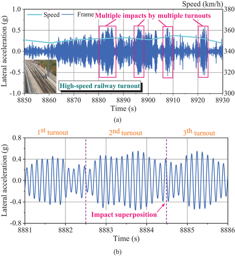
The above-mentioned field test results show that the peak value of the main vibration frequency of CSP vehicles is around 7.90 Hz, which is close to the natural frequency of the diamond-shaped mode of the carbody. The CSPs were exacerbated by the wheel-rail impacts on turnouts. To validate this view, extensive numerical analyses were conducted to reproduce such an abnormal vibration phenomenon and to reveal the mechanism of the HST CSP, which will be presented in the next sections.

3. Numerical modelling

A FE-MBS dynamic model was built to study the mechanism of the CSP. The first step will therefore be to update the carbody FE model, and the second step will be to build on the first step and carry out modelling of the vehicle-track coupled dynamic model.

3.1. FE model updating of the carbody

FE model updating is an important part of numerical simulation of structural engineering. The aim is to calibrate the FE model of the structure, so that the numerical results match the results obtained from modal tests [21–25]. Generally, an accurate model can be obtained by FE modelling for the aluminium structure of the HST carbody, but the HST carbody becomes extremely complex under service environment, and its structure includes not only the aluminium alloy structure of the HST carbody, but also the internal components of the carbody and the various equipment under and inside the carbody. Therefore, based on the measured modal data of the carbody, the model updating work of the carbody under service environment was performed [26,27].

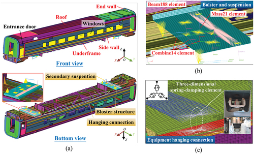
The refined carbody FE model was established by HyperMesh software, and the modal calculation was carried out by ANSYS software. The bolster structure above the bogie was considered for the carbody, and the spring spring-damping force elements (Combine14 element) corresponding to the secondary suspension were established at the bogie bolster (as shown in Figure 6(a)) to bring the FE model closer to the service condition. Figure 6(b,c) show the detailed features of the FE model, i.e. the bolster and secondary suspension system, and the elastic hanging connection of the equipment beneath the underframe. The Mass21 element was used to represent electrical equipment and sewage equipment beneath the vehicle, and provides the related mass and moment of inertia. The RBE3 and Combine14 elements were adopted to simulate the elastic hanging connection of equipment. The FE model is made up of 2,420,442 elements and 1,958,653 nodes, with shell elements being the most important.

Figure 6. Carbody FE model under service environment: (a) Overall view; (b) Bolster and secondary suspension; (c) Equipment hanging connection.

The carbody FE model was calibrated and validated based on experimentally identified modal parameters, namely natural frequencies and mode shapes. The test modal and simulation modal of carbody are judged by modal assurance criterion (MAC) index. $[\mathrm{\Phi }]=\left\{{\varphi }_{1r},{\varphi }_{2r},\begin{array}{c}\cdots \end{array},{\varphi }_{Nr}\right\}$ represent r-th modal vector. Let the r-th modal vector of experimental mode is Φ_r, and the k-th modal vector of computational mode is Φ_k^′. The MAC expression between the two groups of vectors is as follows

(1) $MA{C}_{rk}=\frac{{({{\mathrm{\Phi }}_r}^{t\ast }\mathrm{\Phi }{ }_k^{\prime })}^2}{({{\mathrm{\Phi }}_r}^{t\ast }{\mathrm{\Phi }}_r)(\mathrm{\Phi }{ }_k^{\prime }{{ }^t}^{\ast }\mathrm{\Phi }{ }_k^{\prime })}$(1)

where $t\ast$ stands for conjugate transpose, and the more linearly the two sets of vectors Φ_r,Φ_k^′ are related, the closer the MAC is to 1, which indicates that the k-th experimental mode shape is the same as the r-th calculated mode shape, otherwise, the lower the correlation.

The model was updated based on the concept of equivalent stiffness, which means that the stiffness change of the carbody caused by equipment and interior were taken into account. The carbody was divided into four sections based on the properties of the aluminium alloy structure: underframe, side wall, roof, and end wall. The iterative method was selected to modify the carbody FE model under service environment based on experimental modal parameters. According to the experimental modal parameters, the carbody FE model was modified by iterative method. Figure 7 shows the flow chart of iterative algorithm in the calibration of FE model. As shown in Table 1, the FE modal simulation results are in good agreement with the measured results, and the modal parameters are in agreement with the experimental results. The final parameters are 112.0 GPa for the E_underframe, 55.2 GPa for the E_roof, 66.4 GPa for the E_{side wall}, and 65.7 GPa for the E_{end wall}. The equivalent elastic modulus of each region is not all higher than the 69.0 GPa elastic modulus of aluminium alloy material, and some regions have lower elastic modulus.

Figure 7. FE model updating flow chart.

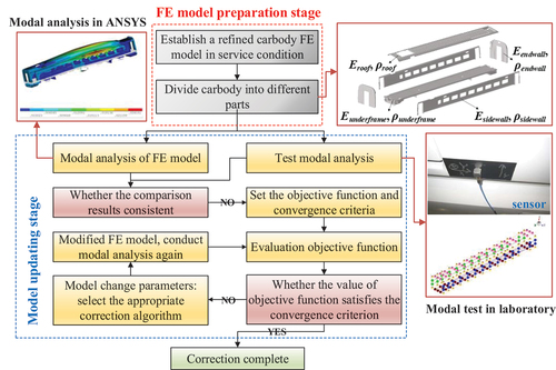
Table 1. Comparison of experimental and simulated modal results.

Mode	Mode of vibration	FEM (Hz)	Test (Hz)	Difference (%)	MAC
1	First-order diamond	8.92	8.73	2.18	0.913
2	First-order respiratory	10.23	9.96	2.71	0.901
3	First-order vertical bending	13.07	12.91	1.24	0.935
4	Second-order diamond	15.25	15.86	3.66	0.883
5	First-order torsion and first order lateral bending	18.36	17.79	3.20	0.895
6	Second-order torsion and second-order lateral bending	18.71	19.04	1.73	0.929

3.2. Vehicle-track coupled dynamics model

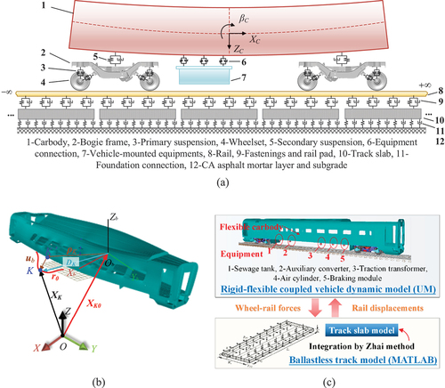
The 3D vehicle-track coupled model reported in the studies of Zhai, Ling et al. and Luo et al. [1,28,29] has been extended to capture the flexible vibration features of HST carriage using the rigid-flexible coupled method. The refined vehicle-track coupled dynamics model is shown in Figure 8(a). The model is composed of a vehicle sub-model with flexible carbody and a slab track sub-model [1]. A wheel-rail contact sub-model as shown in Section 3.2 connects the two sub-models [30,31].

Figure 8. (a) Schematic view of vehicle-track coupled dynamics model; (b) Floating reference frame for carbody; (c) Schematic diagram of co-simulation of vehicle system and track system.

3.2.1. Modelling of flexible carbody

Due to the small elastic deformation of other essential vehicle components and the consideration of reducing calculation time, they were regarded as rigid bodies with six DOFs (longitudinal, lateral, vertical, roll, pitch, and yaw motions) in simulations. We propose a flexible model of the HST carbody based on the FEM and the multibody dynamics (MBD) approaches. The rigid motion of the vehicle is predicted using the MBD theory, and carbody structural deformation is computed using FEM and the modal synthesis approach in the model. In the body-fixed frame of reference, the carbody flexible displacement is expected to be minor and might be represented using linear FE analysis. Incorporating flexible bodies into a mechanical system model allows for the creation of more comprehensive models and more accurate simulation results. The kinematics of the carbody are described with the use of the floating coordinate system O_b-X_bY_bZ_b, as illustrated in Figure 8(b). The global coordinate system O-XYZ position of a specific point K in the carbody is defined by

(2) ${\mathbf{X}}_K={\mathbf{X}}_{K0}+{\mathbf{T}}_{OB}{\mathbf{D}}_K={\mathbf{X}}_{K0}+{\mathbf{T}}_{OB}({\mathbf{u}}_b+\mathit{\rho }{ }_K)$(2)

where X_K0 is radius vector of the origin of O_b-X_bY_bZ_b in O-XYZ, T_OB is transformation matrix, ρ_k is radius vector of point K of undistorted flexible body in O_b-X_bY_bZ_b, vector u_b presents elastic displacements of the point. Small elastic displacements of point K in O_b-X_bY_bZ_b are the product of the modal matrix and the matrix-column of modal coordinates

(3) ${\mathbf{u}}_b(x,y,z,t)=\left[\begin{array}{c}{\mathbf{u}}_{bx}\\ {\mathbf{u}}_{by}\\ {\mathbf{u}}_{bz}\end{array}\right]=\left[\begin{array}{c}\sum _{i=1}^S{\phi }_{ix}(x,y,z)q_i(t)\\ \sum _{i=1}^S{\phi }_{iy}(x,y,z)q_i(t)\\ \sum _{i=1}^S{\phi }_{iz}(x,y,z)q_i(t)\end{array}\right]=\sum _{i=1}^N{\mathrm{\Phi }}_i{q}_i={\mathbf{\Phi }}_b{\mathbf{q}}_b$(3)

where Φ_i is the i-th modal matrix of the carbody, q_i is i-th the modal coordinate that describes flexible displacements. N is referred as the number of used modes. q_b is the overall modal coordinate. Φ_b is called modal matrix which is solved by Craig-Bampton modal synthesis method (CBMSM) [32]. Combining Equations. (2)(2) ${\mathbf{X}}_K={\mathbf{X}}_{K0}+{\mathbf{T}}_{OB}{\mathbf{D}}_K={\mathbf{X}}_{K0}+{\mathbf{T}}_{OB}({\mathbf{u}}_b+\mathit{\rho }{ }_K)$(2) and (3(3) ${\mathbf{u}}_b(x,y,z,t)=\left[\begin{array}{c}{\mathbf{u}}_{bx}\\ {\mathbf{u}}_{by}\\ {\mathbf{u}}_{bz}\end{array}\right]=\left[\begin{array}{c}\sum _{i=1}^S{\phi }_{ix}(x,y,z)q_i(t)\\ \sum _{i=1}^S{\phi }_{iy}(x,y,z)q_i(t)\\ \sum _{i=1}^S{\phi }_{iz}(x,y,z)q_i(t)\end{array}\right]=\sum _{i=1}^N{\mathrm{\Phi }}_i{q}_i={\mathbf{\Phi }}_b{\mathbf{q}}_b$(3) ), the velocity and acceleration vectors of point K on the flexible carbody in the overall coordinate system O-XYZ can be obtained by taking the derivative of time t in Equation (2)(2) ${\mathbf{X}}_K={\mathbf{X}}_{K0}+{\mathbf{T}}_{OB}{\mathbf{D}}_K={\mathbf{X}}_{K0}+{\mathbf{T}}_{OB}({\mathbf{u}}_b+\mathit{\rho }{ }_K)$(2)

(4) $\left\{\begin{array}{c}{\dot{\mathbf{X}}}_K={\dot{\mathbf{X}}}_{K0}+{\dot{\mathbf{T}}}_{OB}({\mathbf{u}}_b+{\rho }_K)+{\mathbf{T}}_{OB}{\mathbf{\Phi }}_b{\dot{\mathbf{q}}}_b\\ {\ddot{\mathbf{X}}}_K={\ddot{\mathbf{X}}}_{K0}+{\ddot{\mathbf{T}}}_{OB}({\mathbf{u}}_b+{\rho }_K)+2{\dot{\mathbf{T}}}_{OB}{\mathbf{\Phi }}_b{\dot{\mathbf{q}}}_b+{\mathbf{T}}_{OB}{\mathbf{\Phi }}_b{\ddot{\mathbf{q}}}_b\end{array}\right.$(4)

According to CBMSM, the displacement of substructures can be divided into the displacement of nodes in the structure and the displacement of nodes at the interface, so the undamped dynamic equation can be written as a block matrix

(5) $\left[\begin{array}{cc}{\mathbf{M}}_i^{{ }_{II}}& {\mathbf{M}}_i^{{ }_{{ }_{BI}}}\\ {\mathbf{M}}_i^{IB}& {\mathbf{M}}_i^{BB}\end{array}\right]\left[\begin{array}{c}{\ddot{\mathbf{u}}}_b^I\\ {\ddot{\mathbf{u}}}_b^B\end{array}\right]+\left[\begin{array}{cc}{\mathbf{K}}_i^{{ }_{II}}& {\mathbf{K}}_i^{{ }_{{ }_{BI}}}\\ {\mathbf{K}}_i^{IB}& {\mathbf{K}}_i^{BB}\end{array}\right]\left[\begin{array}{c}{\mathbf{u}}_b^I\\ {\mathbf{u}}_b^B\end{array}\right]=\left[\begin{array}{c}0\\ {\mathbf{F}}_b^B\end{array}\right]$(5)

where ${\mathbf{M}}_i^{{ }_{II}},{\mathbf{M}}_i^{BB},{\mathbf{K}}_i^{{ }_{II}},{\mathbf{K}}_i^{BB}$ are mass matrix and stiffness matrix at internal and interface of substructure i. ${\mathbf{u}}_b^I,{\mathbf{u}}_b^B$ are the node displacement in substructure and node displacement at interface. ${\mathbf{F}}_b^B$ is the internal force matrix at interface.

(6) ${\mathbf{u}}_b={\mathbf{\Phi }}_b{\mathbf{q}}_b=\left[\begin{array}{c}{\mathbf{u}}_b^I\\ {\mathbf{u}}_b^B\end{array}\right]=\left[\begin{array}{cc}{\mathbf{\Phi }}_n& {\mathbf{\Phi }}_c\end{array}\right]\left[\begin{array}{c}{\mathbf{q}}_b^I\\ {\mathbf{q}}_b^B\end{array}\right]$(6)

where ${\mathbf{\Phi }}_n$ represents the main modal matrix of the fixed interface, which is the modal matrix obtained by fully restricting the fixed interface points; ${\mathbf{\Phi }}_c$ represents the constraint modal matrix, namely the modal matrix obtained by successively releasing each node with each degree of freedom.

The modal matrix obtained by the above equation contains six rigid body modes, which can be clearly separated by matrix transformation of matrix. This is because the rigid body mode is the smallest, which is basically 0, and the smallest six modes can be obtained by matrix transformation. In order to transform the modal matrix in the above process, the eigenvalue analysis is carried out:

(7) $\left\{\begin{array}{c}\left[{\bar{\mathbf{K}}}_i-{\omega }_i^2{\bar{\mathbf{M}}}_i\right]{\mathbf{\Phi }}_b=0\\ {\bar{\mathbf{K}}}_i={\mathbf{\Phi }}_b^T{\mathbf{K}}_i{\mathbf{\Phi }}_b,{\bar{\mathbf{M}}}_i={\mathbf{\Phi }}_b^T{\mathbf{M}}_i{\mathbf{\Phi }}_b\end{array}\right.$(7)

where ω is the frequencies of structure. The original modal coordinates are represented by a new Craig-Bampton modal coordinate. So the physical coordinates can be approximately expressed as

(8) ${\mathbf{u}}_b=\sum _{i=1}^N{\mathrm{\Phi }}_i{q}_i=\sum _{i=1}^N{\mathrm{\Phi }}_i\mathbf{N}{\bar{q}}_i=\sum _{i=1}^N{\bar{\mathrm{\Phi }}}_i{\bar{q}}_i$(8)

where N is the transformation matrix, ${\bar{\mathrm{\Phi }}}_i,{\bar{q}}_i$ are the normalized modal matrix and modal coordinate vector. The carbody damping matrix includes the material damping of the carbody itself and can be given by

(9) $\left\{\begin{array}{c}{\mathbf{C}}_b=\alpha {\bar{\mathbf{M}}}_b+\beta {\bar{\mathbf{K}}}_b\\ \alpha =\frac{2{\xi }_b{\omega }_i{\omega }_j}{{\omega }_i+{\omega }_j},\beta =\frac{2{\xi }_b}{{\omega }_i+{\omega }_j}\end{array}\right.$(9)

where ω_i and ω_j are the natural frequencies of the two flexible modes chosen, and ξ_b is the carbody’s material dependent damping ratio. α and β are the Rayleigh damping coefficients.

In this work, the CBMSM procedure was performed in ANSYS software, and 30 global deformable modes of the carbody were retrieved. The converted carbody FE model has an effective frequency range of 35 Hz, which is suitable for investigating the low and medium frequency vibration response of carbody.

As illustrated in Figure 8(c), the vehicle model is a FE-MBS system with four wheelsets, eight axle boxes, two bogie frames, two bolsters, five vehicle-mounted equipment, one flexible carbody, primary and secondary suspensions. The bogie frames, vehicle-mounted equipment, bolsters, and wheelsets all have six independent DOFs, which, respectively, allow unrestricted movement and rotations in the XYZ directions. Finally, the axle boxes have one degree of freedom in relation to the wheelset (rotation about y-axis). The DOFs of all the vehicle components are listed in Table 2.

Table 2. Degrees of freedom of vehicle system.

Component	Type of motion
	Longitudinal	Lateral	Vertical	Roll	Pitch	Yaw
Bolster (i = 1–2)	Xci	Yci	Zci	ϕci	βci	ψci
Vehicle-mounted equipment (i = 1–5)	Xtri	Ytri	Ztri	ϕtri	βtri	ψtri
Frame (i = 1–2)	Xti	Yti	Zti	ϕti	βti	ψti
Wheelset (i = 1–4)	Xwi	Ywi	Zwi	ϕwi	βwi	ψwi
Axle box (i = 1–4)	–	–	–	–	βmi	–

The Maxwell model, which takes into account the stiffness of the joint and the nonlinear damping behaviour, was used to determine the damping forces of the vehicle suspension systems. The nonlinear spring and damper parts were used to replicate air springs. Special spring and damper elements were used to imitate rubber components and bearings. For example, the elastic connection between on-board equipment and vehicle underframe. The dynamic equilibrium equations of vehicle may be written in the following general form

(10) ${\mathbf{M}}_{tv}{\ddot{\mathbf{X}}}_{tv}+{\mathbf{C}}_{tv}{\dot{\mathbf{X}}}_{tv}+{\mathbf{K}}_{tv}{\mathbf{X}}_{tv}={\mathbf{F}}_{wr}$(10)

where ${\mathbf{X}}_{tv},{\dot{\mathbf{X}}}_{tv},{\ddot{\mathbf{X}}}_{tv}$ represent the displacement, velocity, and acceleration vectors of the vehicle, respectively. M_tv is the mass matrix of the train, C_tv and K_tv are the damping and stiffness matrices, respectively; u_tv is the displacement vector of train components; F_wr is the vector of the nonlinear wheel-rail contact forces. Detailed dynamics equation and its derivation process can be found in Zhai’s study [1].

3.2.2. Modelling of slab track

High-speed railways with running speed of 300 km/h and higher often use ballastless track types. In this study, the dynamics of a slab ballastless track are treated as an object. The ballastless track dynamics model is referenced in the lower part of Figure 8(a). The calculation process of the ballastless track model was completed in MATLAB (see Figure 8(c)) [1]. In the dynamics model, the rails were simplified as Timoshenko beam elements, the differential equations that take into account both shear and rotary inertia effect, the equations written as

(11) $\left\{\begin{array}{c}E{J}_y\frac{{\mathrm{\partial }}^2\psi }{\mathrm{\partial }{x}^2}-k_{z}AG\left(\frac{\mathrm{\partial }\psi }{\mathrm{\partial }x}+\psi \right)-\rho J_y\frac{{\mathrm{\partial }}^2\psi }{\mathrm{\partial }{t}^2}=0\\ E{J}_z\frac{{\mathrm{\partial }}^2\theta }{\mathrm{\partial }{x}^2}+k_{y}AG\left(\frac{\mathrm{\partial }\phi }{\mathrm{\partial }x}-\theta \right)-\rho J_z\frac{{\mathrm{\partial }}^2\theta }{\mathrm{\partial }{t}^2}=0\\ E{J}_{\omega }\frac{{\mathrm{\partial }}^4\phi }{\mathrm{\partial }{x}^4}-G{J}_x\frac{{\mathrm{\partial }}^2\phi }{\mathrm{\partial }{x}^2}-\rho J_{\omega }\frac{{\mathrm{\partial }}^4\phi }{\mathrm{\partial }{x}^2\mathrm{\partial }{t}^2}+\rho z_{s}A\frac{{\mathrm{\partial }}^{2}v}{\mathrm{\partial }{t}^2}-\rho y_{s}A\frac{{\mathrm{\partial }}^{2}w}{\mathrm{\partial }{t}^2}+\rho J_p\frac{{\mathrm{\partial }}^2\phi }{\mathrm{\partial }{t}^2}=\\ M_x(t)\delta [x-x_w(t)]+\sum _{i\in N}\delta (x-x_i^s)M_{x_i}^s(t)\end{array}\right.$(11)

(12) $\left\{\begin{array}{c}EA\frac{{\mathrm{\partial }}^{2}u}{\mathrm{\partial }{x}^2}-\rho A\frac{{\mathrm{\partial }}^{2}u}{\mathrm{\partial }{t}^2}=F_x(t)\delta [x-x_w(t)]+\sum _{i\in N}\delta (x-x_i^s)F_{x_i}^f(t)\\ k_{y}AG\left(\frac{{\mathrm{\partial }}^{2}v}{\mathrm{\partial }{x}^2}-\frac{\mathrm{\partial }\theta }{\mathrm{\partial }x}\right)-\rho A\frac{{\mathrm{\partial }}^{2}v}{\mathrm{\partial }{t}^2}-\rho z_{s}A\frac{{\mathrm{\partial }}^2\phi }{\mathrm{\partial }{t}^2}=F_y(t)\delta [x-x_w(t)]+\sum _{i\in N}\delta (x-x_i^s)F_{y_i}^f(t)\\ k_{z}AG\left(\frac{{\mathrm{\partial }}^{2}w}{\mathrm{\partial }{x}^2}+\frac{\mathrm{\partial }\psi }{\mathrm{\partial }x}\right)-\rho A\frac{{\mathrm{\partial }}^{2}w}{\mathrm{\partial }{t}^2}+\rho y_{s}A\frac{{\mathrm{\partial }}^2\phi }{\mathrm{\partial }{t}^2}=F_z(t)\delta [x-x_w(t)]+\sum _{i\in N}\delta (x-x_i^s)F_{z_i}^f(t)\end{array}\right.$(12)

where E, G are modulus of elasticity and shear modulus, ρ is material density, A is a cross-section area, J_v,J_z are central principal moments of inertia, J_x is St. Venant’s torsional constant, J_w is warping constant, k_y,k_z are shear correction factors in principal planes, J_p is polar moment of inertia, y_s,z_s are coordinates of shear centre relative to centre of gravity in principal central frame of reference, δ is Dirac delta function. θ, ψ, and u are the angular coordinate of the centre of gravity in the YZ direction and the displacement in the X direction. φ, w, and v are the angular coordinate of the shear centre in the X direction and the displacement in the YZ direction. x_w(t) is current longitudinal coordinates of the wheelset, F_x(t), F_v(t), F_z(t) and M_x(t) are longitudinal forces, lateral forces, vertical forces, and relative longitudinal rail axis moment that act on the rail from the wheel, x_i^S are longitudinal coordinates of sleepers.

The fastener system was simplified to a spring-damping system in spatial directions, accounting for the slab ballastless track’s actual force situation. The stiffness and damping matrix K_s-r, C_s-r are respectively

(13) ${\mathit{K}}_{r-s}=\left[\begin{array}{cccccc}{k}_x& \hspace{0.17em}& \hspace{0.17em}& \hspace{0.17em}& \hspace{0.17em}& \hspace{0.17em}\\ \hspace{0.17em}& k_y& \hspace{0.17em}& \hspace{0.17em}& 0& \hspace{0.17em}\\ \hspace{0.17em}& \hspace{0.17em}& k_z& \hspace{0.17em}& \hspace{0.17em}& \hspace{0.17em}\\ \hspace{0.17em}& \hspace{0.17em}& \hspace{0.17em}& k_{ax}& \hspace{0.17em}& \hspace{0.17em}\\ \hspace{0.17em}& 0& \hspace{0.17em}& \hspace{0.17em}& k_{ay}& \hspace{0.17em}\\ \hspace{0.17em}& \hspace{0.17em}& \hspace{0.17em}& \hspace{0.17em}& \hspace{0.17em}& k_{az}\end{array}\right],{\mathit{C}}_{r-s}=\left[\begin{array}{cccccc}{c}_x& \hspace{0.17em}& \hspace{0.17em}& \hspace{0.17em}& \hspace{0.17em}& \hspace{0.17em}\\ \hspace{0.17em}& c_y& \hspace{0.17em}& \hspace{0.17em}& 0& \hspace{0.17em}\\ \hspace{0.17em}& \hspace{0.17em}& c_z& \hspace{0.17em}& \hspace{0.17em}& \hspace{0.17em}\\ \hspace{0.17em}& \hspace{0.17em}& \hspace{0.17em}& c_{ax}& \hspace{0.17em}& \hspace{0.17em}\\ \hspace{0.17em}& 0& \hspace{0.17em}& \hspace{0.17em}& c_{ay}& \hspace{0.17em}\\ \hspace{0.17em}& \hspace{0.17em}& \hspace{0.17em}& \hspace{0.17em}& \hspace{0.17em}& c_{az}\end{array}\right]$(13)

where k_x,k_v,k_z,k_ax,k_ay,k_az are the stiffness in different directions, c_x,c_v,c_z,c_ax,c_ay,c_az are the damping in different directions. The vertical motion of the track slab is reduced to elastic thin slab vibration, and the lateral motion is reduced to rigid body motion; the CA mortar is reduced to Winkler elastic foundation; and the concrete base and substructure are considered rigid boundaries.

3.2.3. Modelling of turnout

In contrast to the main line, the rail cross-section of turnout section will vary with distance, and the structural forms such as rail shape, rail top width, and height will continually change, making force transmission more complicated and increasing vibration influencing variables. A high-speed railway turnout consists of three panels: a switch, a closure, and a crossing (see in Figure 9). The movable elements and varied railhead portions along the switch rail are two key aspects of the switch panel (see partial view (a) in Figure 9).

Figure 9. Schematic diagram of turnout near high-speed railway station.

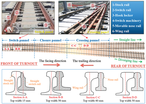
When a train approaches, the crossing panel is a zone where large vertical and lateral loads are exerted. When a train travels over a crossing panel, it exerts significant vertical and lateral forces. On the inner side of the nose rail, near the crossing panel, wing rails have a considerable influence on the wheel-rail rolling contact behaviour and the dynamic interaction of the turnout system. In recent years, scholars have consistently taken into consideration the various cross-section aspects of turnout in order to produce a more realistic turnout model that is more in line with the actual line [33–35].

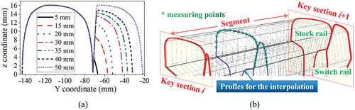
The wheel-rail profile measurement equipment is used to measure the important parts of Chinese No. 18 high-speed turnouts as well as their longitudinal locations along the track, as illustrated in Figure 10(a). The structural forms of spatial turnouts are calculated using discrete data from sections with varying distances. The fitting processing diagram is shown in Figure 10(b), and nonlinear factors such as changes in rail profiles were taken into account in the turnout model.

Figure 10. (a) Key sections of switch rail; (b) Schematic diagram of key sections fitting method.

3.2.4. Modelling of wheel-rail contact

The normal and tangential forces in the wheel-rail contact region are generally comparable in the wheel-rail interaction. The Kik-Piotrowski model for wheel-rail contact is non-elliptical multi-point contact model based on the virtual penetration contact theory [30,31], which assumes that the form of the contact site is directly dictated by the wheel-rail profile and the degree of indentation. The Kik-Piotrowski model solves for the wheel-rail contact patch normal force N, moment of the normal force M and the maximum pressure p₀ can be calculated as follows:

(14) $N=\frac{\pi E{\delta }_0}{2(1-{\mu }^2)}\frac{{\int }_{y_r}^{y_l}{\int }_{-x_l(y)}^{x_l(y)}\sqrt{x_l{(y)}^2-x^2}dxdy}{{\int }_{y_r}^{y_l}{\int }_{-x_l(y)}^{x_l(y)}\sqrt{\frac{x_l{(y)}^2-x^2}{x^2+y^2}}dxdy}$(14)

(15) $M=\frac{p_0}{x_l(0)}{\int }_{y_r}^{y_l}{\int }_{-x_l(y)}^{x_l(y)}\sqrt{x_l{(y)}^2-x^2}dxdy$(15)

(16) $p_0=\frac{N\sqrt{2R{\delta }_0}}{{\int }_{y_r}^{y_l}{\int }_{-x_l(y)}^{x_l(y)}\sqrt{x_l{(y)}^2-x^2}dxdy}$(16)

where δ₀ is the amount of penetration at the centre of the contact patch, x_l(y) are the coordinates of the left edge of the contact area, E, μ are the elastic parameter of the material and R is the principal radius of curvature of the wheel profile at the point of contact.

The tangential force is solved using the FASTSIM technique. The FASTSIM algorithm is a general approach in that sense that its application area is not limited to the elliptical contact, but it can be used for an arbitrary area of contact. In such case, there is difficulty in computing compliance coefficients, since they are only well defined for elliptic area of contact. The modified FASTSIM algorithm was therefore used to solve for the tangential forces

(17) $\left\{\begin{array}{c}{F}_x={\int }_{y_r}^{y_l}{\int }_{-x_l}^{x_l}{q}_x(x,y)dxdy=-\frac{4R}{L_1}{\xi }_x{\int }_{y_r}^{y_l}g(y)dy+\frac{4R}{L_3}\psi {\int }_{y_r}^{y_l}yg(y)dy\\ F_y={\int }_{y_1}^{y_2}{\int }_{-x_l}^{x_l}{q}_y(x,y)dxdy=-\frac{4R}{L_2}{\xi }_y{\int }_{y_r}^{y_l}g(y)dy+\frac{4\sqrt{2}}{3L_3}\psi {\int }_{y_r}^{y_l}{[Rg(y)]}^{\frac{3}{2}}dy\end{array}\right.$(17)

where Ψ is the spin, ξ_x,ξ_y are the longitudinal and lateral creepages. The interpenetration function g(y) is defined to be

(18) $g(y)=\left\{\begin{array}{c}{\delta }_0-h(y),h(y)\le {\delta }_0\\ 0(y)>{\delta }_0\end{array}\right.$(18)

where the compliance parameters can be found by equalling the resulting tangent loads to the creep forces obtained according to the linear theory of rolling contact

(19) $\left\{\begin{array}{c}{L}_1=\frac{4\pi R}{GA{C}_{11}}{\int }_{y_r}^{y_l}g(y)dy\\ L_2=\frac{4\pi R}{GA{C}_{22}}{\int }_{y_r}^{y_l}g(y)dy\\ L_3=\frac{4\sqrt{2{\pi }^3{R}^3}}{G{A}^{3/2}{C}_{23}}{{\int }_{y_r}^{y_l}g(y)}^{3/2}dy\end{array}\right.$(19)

where coefficients of creep and spin C_ij are tabulated using data of an equivalent elliptic area of contact as parameters.

3.3. Numerical integration method

As depicted in Figure 8(c), the track system and the vehicle system are solved independently in this paper, with the two independent systems using rail displacement and wheel-rail force as iterative exchange intermediate variables to complete the solution of the dynamics equations for the whole system. For multi-degree-of-freedom nonlinear time-varying dynamical systems, the numerical integration method is generally used to solve them. In this paper, a new fast explicit integration method (Zhai method [36]) is used to solve the system of differential equations for the dynamics of track systems in the following integration format

(20) $\left\{\begin{array}{c}{\mathbf{X}}_{n+1}={\mathbf{X}}_n+{\dot{\mathbf{X}}}_n\mathrm{\Delta }t+(0.5+\psi ){\ddot{\mathbf{X}}}_n\mathrm{\Delta }{t}^2-\psi {\ddot{\mathbf{X}}}_{n-1}\mathrm{\Delta }{t}^2\\ {\dot{\mathbf{X}}}_{n+1}={\dot{\mathbf{X}}}_n+(1+\varphi ){\ddot{\mathbf{X}}}_n\mathrm{\Delta }t-\varphi {\ddot{\mathbf{X}}}_{n-1}\mathrm{\Delta }t\end{array}\right.$(20)

where Δt is the time integration step; n represents the number of integration steps; ψ and φ are independent parameters controlling the characteristics of the integration method and are generally taken to be 0.5.

In contrast, the vehicle dynamics equations for the rigid-flexible system are solved using the Park integral method [37]

(21) $\left\{\begin{array}{c}{\dot{\mathbf{X}}}_{n+1}=(6\mathrm{\Delta }t{)}^{-1}(10{\mathbf{X}}_{n+1}-15{\mathbf{X}}_n+6{\mathbf{X}}_{n-1}-{\mathbf{X}}_{n-2})\\ {\ddot{\mathbf{X}}}_{n+1}=(6\mathrm{\Delta }t{)}^{-1}(10{\dot{\mathbf{X}}}_{n+1}-15{\dot{\mathbf{X}}}_n+6{\dot{\mathbf{X}}}_{n-1}-{\dot{\mathbf{X}}}_{n-2})\end{array}\right.$(21)

The integration steps for both methods take the value 10⁻⁴ s. The vehicle model and the track model are jointly calculated by interacting rail displacement and wheel-rail force.

4. Numerical results and discussion on CSP

To investigate the influence of wheel-rail wear profiles on the HST CSP, the numerical simulations in Section 4 were carried out in terms of wheel-rail wear profiles and turnout impacts. The wheel-rail profiles were collected from the measured profiles of vehicles or railway lines where CSP occurred in the field, and the turnout key section data were taken from the turnout design drawings.

4.1. Influence of wheel-rail wear profiles

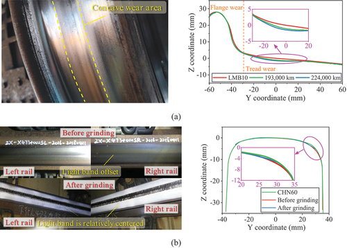
A static analysis of wheel-rail contact geometric relationship on the main line section was first carried out. Figure 11 shows that after 193,000 km and 224,000 km, there are obvious concave wear areas on the wheels, mainly in the range of −20 mm to 20 mm, accompanied by a certain degree of rim wear, as shown by collecting wheel profiles during the vehicle shaking period and rail profiles on some sections where CSP occurred. The maximum wear depth near the wheel nominal rolling circle is 1.44 mm. The rail profiles were checked twice: once before CSP, when the rail was unpolished, and again after it had been trimmed, ground, and polished. Further examination of the site rail profiles reveals that:

1. Before grinding, the average width of the light bands is 37.5 mm, about 11.6 mm from the inner working edge and 20.9 mm from the outer non-working edge.

2. After grinding, the rail left and right light bands are 20 mm wide. The width is moderate and uniform, kept in the middle, and the left and right strands have good symmetry. The height of rail shoulder is reduced, which can reduce the equivalent conicity matching with the worn wheel profile (WWP).

Figure 11. Measured wheel and rail profiles: (a) Wheel profiles; (b) Rail profiles

S

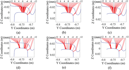
The WWP (224,000 km) and the standard wheel profile (SWP) were selected for static contact geometry analysis, where the rail profiles before and after grinding and the standard CHN60 rail profiles (abbreviated as BGRP, AGRP, and SRP in turn) were considered. According to the distribution of contact lines in Figure 12, the distribution of contact points on the wheel is very concentrated for typical wheel-rail profile matching, and with the lateral movement of wheelsets, the distribution moves quite steadily. The distribution of contact lines, which matches the profile before grinding, is unaffected by changes in rail profile, and the distribution of contact points is broader towards the gauge angle. The wheel concave wear profile is more influenced by the rail profile before grinding. Concave wear will lead to multi-point contact distribution on the rail top surface, resulting in conformal contact and amplifying wheel-rail interaction, as shown in Figure 12(e) for WWP. There is a ”jump” in the distribution of contact points on the WWP. The distribution of contact points on wheels is more dispersed than that on the SWP.

Figure 12. Wheel-rail contact pairs: (a) SWP-CHN60; (b) SWP-BGRP; (c) SWP-AGRP; (d) WWP-CHN60; (e) WWP-BGRP; (f) WWP-AGRP.

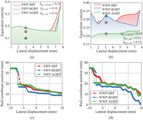
Figure 13 gives the results of the wheel-rail contact geometry analysis for matching the standard and abrasive wheel profiles with different types of rail profiles. The UIC519 technique is used to calculate equivalent conicity. Figure 13(a) shows that WRP reduces the nominal equivalent taper (3 mm location in curve) of SWP from 0.15 to 0.10, but after grinding, the equivalent conicity value soon returns to the SWP-SRP situation. In contrast, as shown in Figure 13(b), following the concave wear of the wheel, the equivalent conicity of the wheel and rail will grow greatly, while the abnormal wear of the rail will further increase the equivalent conicity, and the maximum value might approach 0.33. The distribution of contact point coordinates on the rail top surface for various wheel-rail matches is shown in Figure 13(c,d).

Figure 13. Geometric analysis of wheel-rail contact: (a) Equivalent conicity of SWP; (b) Equivalent conicity of WWP; (c) Rail coordinate position of SWP; (d) Rail coordinate position of WWP.

The curve of standard wheel-rail profile matching is considerably more pronounced, while the curve of standard wheel-rail profile matching is much flatter. It is simple to obtain the hunting motion frequency formula of wheelsets under free and full stiff restrictions using nominal equivalent conicity values and hunting motion Equation. (22)(22) $\left\{\begin{array}{c}{L}_t=\frac{1}{2\pi }\sqrt{\frac{b{r}_0}{\lambda }\left(\frac{b^2+L_b^2}{b^2}\right)},\begin{array}{c}\hspace{0.17em}\end{array}{L}_w=L_t\sqrt{\frac{b^2}{b^2+L_b^2}}\\ f_t=\frac{v_c/3.6}{L_t},\begin{array}{c}\hspace{0.17em}\end{array}{f}_w=\frac{v_c/3.6}{L_w}\end{array}\right.$(22) .

(22) $\left\{\begin{array}{c}{L}_t=\frac{1}{2\pi }\sqrt{\frac{b{r}_0}{\lambda }\left(\frac{b^2+L_b^2}{b^2}\right)},\begin{array}{c}\hspace{0.17em}\end{array}{L}_w=L_t\sqrt{\frac{b^2}{b^2+L_b^2}}\\ f_t=\frac{v_c/3.6}{L_t},\begin{array}{c}\hspace{0.17em}\end{array}{f}_w=\frac{v_c/3.6}{L_w}\end{array}\right.$(22)

where L_t represents the hunting wavelength of wheelset under rigid bogie positioning, f_t is the corresponding frequency; L_w represents the hunting wavelength of wheelset under free bogie positioning, f_w is the corresponding frequency; L_b is half of the bogie wheelbase, b is half of the nominal rolling circle distance of the wheels on the left and right side of the wheelset, and v_c is the train running speed.

In practice, due to the elastic positioning of the wheelset, the actual hunting motion wavelength L_e falls somewhere in between varying with speed

(23) $L_e=L_w\sqrt{1+(\frac{L_b}{b})(1-\eta )}$(23)

where η is the influence of the wavelength L_w and the σ and Z required to calculate δ are determined by Equations 22(22) $\left\{\begin{array}{c}{L}_t=\frac{1}{2\pi }\sqrt{\frac{b{r}_0}{\lambda }\left(\frac{b^2+L_b^2}{b^2}\right)},\begin{array}{c}\hspace{0.17em}\end{array}{L}_w=L_t\sqrt{\frac{b^2}{b^2+L_b^2}}\\ f_t=\frac{v_c/3.6}{L_t},\begin{array}{c}\hspace{0.17em}\end{array}{f}_w=\frac{v_c/3.6}{L_w}\end{array}\right.$(22) –23(23) $L_e=L_w\sqrt{1+(\frac{L_b}{b})(1-\eta )}$(23)

(24) $\left\{\begin{array}{c}\eta =\frac{(1-\sigma Z)}{1+Z^2}\\ \sigma =(2p-3){\beta }^2,\begin{array}{c}\hspace{0.17em}\end{array}Z=\beta K^p\end{array}\right.$(24)

(25) $\left\{\begin{array}{c}\beta =\frac{b}{L_b},\begin{array}{c}\hspace{0.17em}\end{array}p=1+\frac{k_{p\psi }}{k_{p\psi }+k_{py}{L}_b^2}\\ K=\frac{L_w}{2\pi f_{creep}{b}^2}\frac{k_{p\psi }{k}_{py}{L}_b^2}{k_{p\psi }+k_{py}{L}_b^2}\end{array}\right.$(25)

where k_pψ represents yaw stiffness of primary suspension, k_py is lateral stiffness of primary suspension, f_creep is a comprehensive creep coefficient, which is related to the wheel-rail contact patch. According to the definition, 1 ≤ p ≤ 2, and σ and Z are single increasing functions. It is easy to deduce 0 ≤ δ ≤ 1, f_t ≤ f_e ≤ f_w. The lateral stiffness of the high-speed bogie wheelset studied in the paper is 919.8 kN/m, the primary suspension springs with a lateral span of 2 m and k_py of 919.8 kN.m/rad, L_b = 1.25 m, b = 0.7465 m, associating Equations 22(22) $\left\{\begin{array}{c}{L}_t=\frac{1}{2\pi }\sqrt{\frac{b{r}_0}{\lambda }\left(\frac{b^2+L_b^2}{b^2}\right)},\begin{array}{c}\hspace{0.17em}\end{array}{L}_w=L_t\sqrt{\frac{b^2}{b^2+L_b^2}}\\ f_t=\frac{v_c/3.6}{L_t},\begin{array}{c}\hspace{0.17em}\end{array}{f}_w=\frac{v_c/3.6}{L_w}\end{array}\right.$(22) –25(25) $\left\{\begin{array}{c}\beta =\frac{b}{L_b},\begin{array}{c}\hspace{0.17em}\end{array}p=1+\frac{k_{p\psi }}{k_{p\psi }+k_{py}{L}_b^2}\\ K=\frac{L_w}{2\pi f_{creep}{b}^2}\frac{k_{p\psi }{k}_{py}{L}_b^2}{k_{p\psi }+k_{py}{L}_b^2}\end{array}\right.$(25) , f_creep in accordance with the literature [5] suggests taking the average value of the wheel longitudinal creep coefficient and lateral creep coefficient, here 1.36. See Table 3 for the corresponding calculation results. Table 3 clearly shows that the hunting motion frequency of the elastic positioned bogie is approximately the DM frequency of the carbody for nominal equivalent conicity of 0.28 and 0.33.

Table 3. Cause classification of hunting motion frequency of bogie.

No.	Wheel-rail matching type	Equivalent conicity (3 mm position)	Rigid positioned bogie	Elastic positioned bogie
1	SWP-SRP	0.15	5.24	5.83
2	SWP-BGRP	0.10	4.28	4.88
3	SWP-AGRP	0.16	5.41	6.22
4	WWP-SRP	0.28	7.16	7.72
5	WWP-BGRP	0.33	7.78	8.31
6	WWP-AGRP	0.22	6.35	6.97

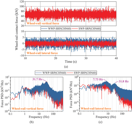
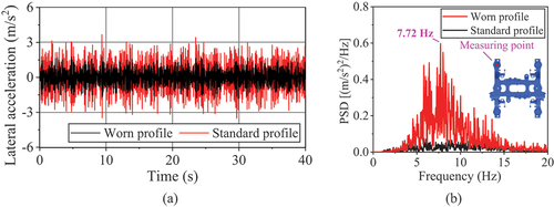
Then, numerical simulation was carried out by using the rigid-flexible coupled dynamic model mentioned above. When CSP occurred, the railway random irregularity was modelled using the China high-speed ballastless railway spectrum, the simulation distance was set to 4,000 m, and the vehicle speed was set to 350 km/h. Figure 14 depicts time histories and PSD comparison of wheel-rail contact forces for WWP and SWP under the CHN60 rail profile. The wheel-rail vertical forces are mostly unaffected by concave wheel wear, but the lateral forces are significantly affected. SWP creates strong peaks at 7.73 Hz and 31.8 Hz frequencies in the lateral direction, with a considerable increase in the mid- and high-frequency components, as seen in PSD comparison diagrams. SWP has practically negligible influence in the low- and mid-frequency sections of the vertical direction.

Figure 14. Simulation results of wheel-rail force: (a) Time domain; (b) PSD of wheel-rail vertical force; (c) PSD of wheel-rail lateral force.

Figure 15(a,b) clearly shows that WWP has a remarkable effect on the vibration performance of the carbody middle floor in both vertical and lateral directions, with the vertical maximum acceleration jumping from 0.444 m/s² to 0.604 m/s² and the root mean square value doubling from 0.0512 m/s² to 0.106 m/s². The lateral maximum acceleration increases from 0.175 m/s² to 0.376 m/s² and the root mean square increases from 0.0993 m/s² to 0.181 m/s². For the convenience of comparison and analysis, the calculation results of WWP and SWP are plotted on the time-frequency diagram in Figure 15(c,d). According to the CWT diagrams, it can be clearly seen that when the WWP is near 8 Hz, the area of energy concentration is obviously darker than SWP. At the same time, the colour depth in the CWT diagram is also related to the track factors such as the amplitude and wavelength of the track irregularity.

Figure 15. Simulation results of middle floor: (a) Time domain of vertical acceleration; (b) Time domain of lateral acceleration; (c) CWT of vertical acceleration; (d) CWT of lateral acceleration.

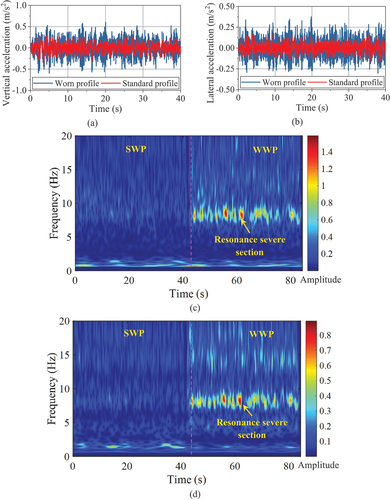
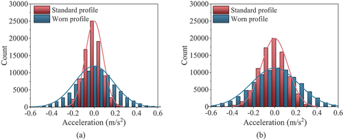
This section of the simulation demonstrates that the frequency of hunting motion generated by wheel concave abrasion causes elastic resonance in the vehicle carbody, and that the effect is stronger in the vertical direction than in the lateral direction, which matches the field test findings. The statistical distribution in Figure 16 shows that WWP results in more data dispersion, flatter distribution curves, and a reduction in the quantity of data around the zero mean.

Figure 16. Distribution comparison diagram of carbody middle floor acceleration: (a) Vertical; (b) Lateral.

The time domain and frequency domain diagrams for the lateral acceleration of the bogie frame are shown in Figure 17. The bogie hunting motion frequency under concave wheel wear is 7.72 Hz in the spectrum, which is near to the carbody DM frequency and is the fundamental cause of the peak in carbody acceleration at 8 Hz. This further confirms that the 8 Hz peak frequency that appears on the floor of the carbody is the cause of the hunting of the bogie.

Figure 17. Bogie frame lateral acceleration: (a) Time-domain; (b) PSD.

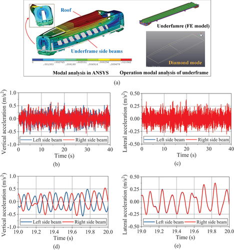
Due to the diamond-shaped deformation of the carbody, the underframe side beams in the middle of the carbody and the left and right sides of the carbody roof are the most obvious (see in Figure 18(a)). In order to further determine that the carbody has diamond deformation, the acceleration time history curves of the left- and right-side beams of the underframe were also investigated in the simulation. The results shown in Figure 18(c-e) suggest that the vertical vibration of the side beams is in the same direction, and the lateral vibration is opposite, which belongs to the typical DM deformation feature. The results in Figures 14 to 18 are analysed primarily in terms of wheel material wear, and from previous test work [38] and [39–42] it is clear that the condition of the rail profile can also play a crucial role in the dynamic performance of the vehicle.

Figure 18. Time-domain of carbody underframe side beam accelerations: (a) Operation modal test; (b) Vertical acceleration; (c) Lateral acceleration; (d) Partial enlargement of Figure (a); (e) Partial enlargement of Figure (c).

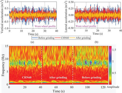
Figure 19 compares the impact of different rail profiles on CSP. The wheel profiles were uniformly set by WWP. Combined with the previous results of wheel-rail contact geometry analysis, the wheel-rail profile matching under BGRP deteriorates further, resulting in a hunting frequency closer to the DM frequency of the carbody, thus aggravating the CSP. Grinding the rail can effectively reduce the vibration amplitude of the carbody, and the overall fluctuation can be reduced by half as shown in Figure 19(a,b). According to the time-frequency diagram in Figure 19(c), the carbody floor acceleration after grinding becomes lighter near 8 Hz, which proves that CSP is relieved. By grinding the rail in a planned way, the wheel-rail equivalent conicity can be reduced and the matching relationship between wheel and rail can be improved.

Figure 19. Comparison diagrams of middle floor accelerations before and after rail grinding: (a) Time-domain; (b) PSD.

4.2. Influence of wheel-rail impact at turnout

This sub-section further investigates the dynamic response of a vehicle straight passing through a multiple turnout sections at high-speed. According to the No. 18 turnout design specification, the passing speed is 350 km/h. In order to highlight the influence of inherent structural irregularity of turnout and due to the good maintenance of line conditions near the station, the influence of conventional track irregularity was not considered in this simulation.

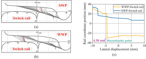
Figure 20(a,b) give the wheel-switch rail geometrical contact relationships in switch panel with top width with 35 mm of SWP and WWP, respectively. A clear difference in the distribution of the contact lines between the WWP and SWP can be clearly observed in the diagram. Due to concave abrasion of WWP, the contact point will jump to the left on the stock rail, which is distributed jointly on the stock rail and switch point rail. Figure 20(c) describes the comparison curves of SWP and WWP at the rail coordinate position after matching with the switch rail. WWP has obvious jump phenomenon and evident fluctuation when the wheelset displacement is equal to 4.30 mm, while SWP has the first jump at 7.80 mm, but the jump amplitude is much smaller than WWP.

Figure 20. (a) SWP-Switch rail with top width of 35 mm; (b) WWP-Switch rail with top width of 35 mm; (c) Rail coordinate position of WWP-Switch rail.

In order to simulate the vibration response of a train passing through multiple turnout sections at high speed in a straight direction, based on the actual layout of the turnouts at the station. Figure 21(a,b) depict the two turnout layouts adopted in this study, Type A and Type B. In the simulation, a total of four turnouts were set in the order of A-B-A-B, and the second and third turnouts are closer to each other. Figure 21(c,d) presents the characteristics of the vertical and lateral acceleration signals in the middle floor when passing through this section at a high speed of 350 km/h. It is evident to observe that the floor was subject to the continuous impact effect of the unevenness of the turnout structure, and the WWP aggravates the impact response of the vehicle passing through the turnout at high speed. The vertical and lateral acceleration peaks of the floor can reach 0.76 m/s² and 0.53 m/s², respectively.

Figure 21. Type of turnout layout and middle floor acceleration: (a) Type A; (b) Type B; (c) Vertical; (d) Lateral.

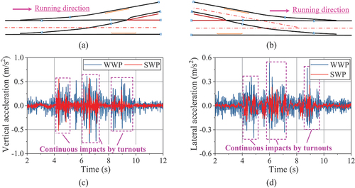
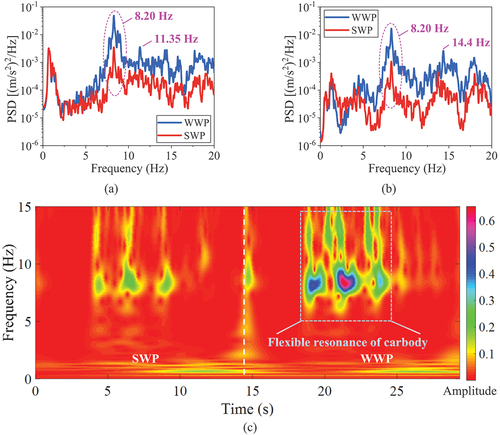
Figure 22(a,c) show that when the vehicle passing through many turnouts at high speeds, the turnout structure may cause elastic deformation of the vehicle carbody, which appears in the energy concentration area of about 8.20 Hz for both SWP and WWP. On the other hand, WWP may amplify the CSP to a certain extent, resulting in a larger peak in the dominant frequency.

Figure 22. Middle floor acceleration: (a) PSD of vertical acceleration; (b) PSD of lateral acceleration; (c) CWT of vertical acceleration under SWP and WWP condition.

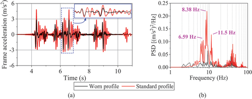
The time-domain and frequency-domain analysis diagram of bogie frame lateral acceleration is shown in Figure 23. The frame is clearly vibrated harmonically by WWP, and the spectrum diagram can be easily detected. At this point, the bogie hunting motion frequency of 8.38 Hz is highly noticeable. The frequencies of 6.59 Hz and 11.5 Hz represent the roll motion of front and rear wheelset of bogie and the pitch motion of frame.

Figure 23. Bogie frame lateral acceleration: (a) Time-domain; (b) PSD.

5. Conclusions and outlook

This paper reported the mechanism of the CSP of an HST in Chinese high-speed railway. The vibration characteristics, wheel-rail contact geometry, and geographical location of the newly discovered CSPs were systematically tested on site. Based on the vehicle-track coupled dynamics theory and CBMSM, a rigid-flexible coupled dynamics model was established to reproduce the CSP of the HST on a real high-speed railway line. Hence, the following conclusions are drawn:

1. A FE model updating approach that combined measured modal data with simulation modal data was applied to build the rigid-flexible coupled dynamics model. The modal updating process ensures the accuracy of the carbody FE model. CSP modelling depends on an accurate carbody FE model.

2. The worn wheel-rail profiles have a significant influence on the CSP, and CSP is easy to appear in the case of worn rail and concave worn wheel. The appearance of the CSP on the railway main line is mainly related to the deterioration of wheel-rail contact geometry. This means that the wheel-rail contact geometry should be inspected in time to avoid the development of the CSP.

3. The combination of the wheel-rail impacts in multiple turnout sections and the WWP will aggravate the CSP when HST passing through railway stations. In order to avoid serious CSP in turnout area, it is a possible countermeasure to appropriately reduce the running speed of HST passing through the station.

The CSP suppression strategies are ongoing, from the viewpoints of maintaining a healthy wheel-rail contact geometry and optimal design of HST carbody structure, as well as conducting field trials to verify the effectiveness of the countermeasures.

Highlights

• The vibration feature of high-speed train (HST) carbody shaking phenomenon (CSP) is presented;

• A three-dimensional rigid-flexible coupled dynamic model for HST is constructed;

• The mechanism and root cause of the CSP occurring on a type of HST are revealed;

• The CSP is mainly caused by the vehicle system resonance induced by deterioration of wheel-rail contact geometry;

• Wheel-rail impacts at turnouts can aggravate the CSP of HSTs.

Acknowledgments

The authors wish to thank all the staff members involved in the field test at the CRRC Changchun Railway Vehicle Co., Ltd., Changchun, China.

Disclosure statement

No potential conflict of interest was reported by the author(s).

Additional information

Funding

This work was supported by the National Natural Science Foundation of China [grant numbers 51735012, U19A20110, 52072317], [grant number B16041], and the Key Science and Technology Projects of CRRC [grant No. 2020CYB147].

References

- Zhai W. Vehicle-track coupled dynamics: theory and applications. Singapore: Springer Nature; 2020.
- Jing L, Wang KY, Zhai WM. Impact vibration behavior of railway vehicles: a state-of-the-art overview. Acta Mech Sin. 2021;37(8):1193–1221.
- Wei L, Zeng J, Chi M, et al. Carbody elastic vibrations of high-speed vehicles caused by bogie hunting instability. Vehicle Syst Dyn. 2017;55(9):1321–1342.
- Shi H, Wu P. Flexible vibration analysis for car body of high-speed EMU. J Mech Sci Technol. 2016;30(1):55–66.
- Li F, Wu H, Liu C, et al. Vibration fatigue analysis of high-speed railway vehicle carbody under shaking condition. Vehicle Syst Dyn. 2021;1–21. doi:10.1080/00423114.2021.1880013
- Qi Y, Dai H, Song C, et al. Shaking analysis of high-speed train’s carbody when cross lines. J Mech Sci Technol. 2019;33(3):1055–1064.
- Morales AL, Chicharro JM, Palomares E, et al. Experimental analysis of the influence of the passengers on flexural vibrations of railway vehicle carbodies. Vehicle Syst Dyn. 2021;1–20. DOI:10.1080/00423114.2021.1927119
- Yang Y, Ling L, Liu P, et al. Experimental investigation of essential feature of polygonal wear of locomotive wheels. Measurement. 2020;166:108199.
- Tao G, Wen Z, Jin X, et al. Polygonisation of railway wheels: a critical review. Railway Eng Sci. 2020;28(4):317–345.
- Sun J, Chi M, Jin X, et al. Experimental and numerical study on carbody hunting of electric locomotive induced by low wheel-rail contact conicity. Vehicle Syst Dyn. 2021;59(2):203–223.
- Xia Z, Zhou J, Gong D, et al. On the modal damping abnormal variation mechanism for railway vehicles. Mech Syst Signal Proc. 2019;122:256–272.
- Gong D, Liu G, Zhou J. Research on mechanism and control methods of carbody chattering of an electric multiple-unit train. Multibody Syst Dyn. 2021;53(2):135–172.
- Tomioka T, Takigami T. Reduction of bending vibration in railway vehicle carbodies using carbody-bogie dynamic interaction. Vehicle Syst Dyn. 2020;48(S1):467–486.
- Huang C, Zeng J. Suppression of the flexible carbody resonance due to bogie instability by using a DVA suspended on the bogie frame. Vehicle Syst Dyn. 2021;1–20. DOI:10.1080/00423114.2021.1930071
- Yang S, Li F, Shi H, et al. A roll frequency design method for underframe equipment of a high-speed railway vehicle for elastic vibration reduction. Vehicle Syst Dyn. 2021;1–20. doi:10.1080/00423114.2021.1899252
- Gong D, Duan Y, Wang K, et al. Modelling rubber dynamic stiffness for numerical predictions of the effects of temperature and speed on the vibration of a railway vehicle car body. J Sound Vibr. 2019;449:121–139.
- Chen X, Yao Y, Shen L, et al. Multi-objective optimization of high-speed train suspension parameters for improving hunting stability. Int J Rail Transp. 2021;10(2):159–176.
- Yao Y, Li G, Wu G, et al. Suspension parameters optimum of high-speed train bogie for hunting stability robustness. Int J Rail Transp. 2020;8(3):195–214.
- Alizadeh Kaklar J, Ghajar R, Tavakkoli H. Modelling of nonlinear hunting instability for a high-speed railway vehicle equipped by hollow worn wheels. Proc Inst Mech Eng Pt K-J Multi-Body Dyn. 2016;230(4):553–567.
- Polach O, Nicklisch D. Wheel/rail contact geometry parameters in regard to vehicle behavior and their alteration with wear. Wear. 2016;366:200–208.
- Girardi M, Padovani C, Pellegrini D, et al. A finite element model updating method based on global optimization. Mech Syst Signal Proc. 2021;152:107372.
- Zhu H, Li J, Tian W, et al. An enhanced substructure-based response sensitivity method for finite element model updating of large-scale structures. Mech Syst Signal Proc. 2021;154:107359.
- Mukesh K, Rodrigo A, Ramin M, et al. Bayesian updating and identifiability assessment of nonlinear finite element models. Mech Syst Signal Proc. 2022;167:108517.
- Zanarini A. Full field optical measurements in experimental modal analysis and model updating. J Sound Vibr. 2019;442:817–842.
- Tian W, Weng S, Xia Y. Model updating of nonlinear structures using substructuring method. J Sound Vibr. 2022;521:116719.
- Li F, Wu H, Wu P. Vibration fatigue dynamic stress simulation under non-stationary state. Mech Syst Signal Proc. 2021;146:107006.
- Akiyama Y, Tomioka T, Takigami T, et al. A three-dimensional analytical model and parameter determination method of the elastic vibration of a railway vehicle carbody. Vehicle Syst Dyn. 2020;58(4):545–568.
- Ling L, Zhang Q, Xiao X, et al. Integration of car-body flexibility into train-track coupling system dynamics analysis. Vehicle Syst Dyn. 2018;56(4):485–505.
- Luo J, Zhu S, Zhai W. An advanced train-slab track spatially coupled dynamics model: theoretical methodologies and numerical applications. J Sound Vibr. 2021;501:116059.
- Sun Y, Zhai W, Ye Y, et al. A simplified model for solving wheel-rail non-hertzian normal contact problem under the influence of yaw angle. Int J Mech Sci. 2020;174:105554.
- Piotrowski J, Kik W. A simplified model of wheel/rail contact mechanics for non-Hertzian problems and its application in rail vehicle dynamic simulations. Vehicle Syst Dyn. 2008;46(1–2):27–48.
- Boo SH, Kim JH, Lee PS. Towards improving the enhanced Craig-Bampton method. Comput Struct. 2018;196:63–75.
- Xu L, Liu X. Matrix coupled model for the vehicle-track interaction analysis featured to the railway crossing. Mech Syst Signal Proc. 2021;152:107485.
- Jing G, Siahkouhi M, Qian K, et al. Development of a field condition monitoring system in high speed railway turnout. Measurement. 2021;169:108358.
- Ge X, Ling L, Guo L, et al. Dynamic derailment simulation of an empty wagon passing a turnout in the through route. Vehicle Syst Dyn. 2022;60(4):1148–1169.
- Zhai W. Two simple fast integration methods for large-scale dynamic problems in engineering. Int J Numer Methods Eng. 1996;39(24):4199–4214.
- Pogorelov D. Differential–algebraic equations in multibody system modeling. Numer Algorithms. 1998;19(1):183–194.
- Zhai W, Liu P, Lin J, et al. Experimental investigation on vibration behaviour of a CRH train at speed of 350 km/h. Int J Rail Transp. 2015;3(1):1–16.
- Ye Y, Vuitton J, Sun Y, et al. Railway wheel profile fine-tuning system for profile recommendation. Railway Eng Sci. 2021;29(1):74–93.
- Torstensson PT, Nielsen JC, Baeza L. Dynamic train-track interaction at high vehicle speeds-Modelling of wheelset dynamics and wheel rotation. J Sound Vibr. 2011;330(22):5309–5321.
- Xu K, Feng Z, Wu H, et al. Investigating the influence of rail grinding on stability, vibration, and ride comfort of high-speed EMUs using multi-body dynamics modelling. Vehicle Syst Dyn. 2018;57(11):1621–1642.
- Cuervo PA, Santa JF, Toro A. Correlations between wear mechanisms and rail grinding operations in a commercial railroad. Tribol Int. 2015;82:265–273.