Experimental validation of a non-linear train-track-bridge dynamic model of a stone arch railway bridge under freight traffic

ABSTRACT

This article presents the validation of a non-linear FE numerical model of a multi-span stone arch railway bridge based on experimental tests and under in-service freight trains. Static loading tests allow evaluating the bridge response in terms of vertical displacements in the arches, opening/closure deformations on specific block joints of the arches, and vertical compressive stress variations in the piers.      The bridge FE model is developed by combining the potentialities of a global continuous homogeneous model, based on FEM and Drucker-Prager model, and a local modelling approach based on a dedicated non-linear contact model. The freight vehicle modelling is based on a flexible FE approach, and the validation of the dynamic behaviour of the train-bridge system involved the comparison between numerical and experimental responses. All the numerical responses are in very good agreement with the experimental responses. Finally, a simulation of the dynamic behaviour of the train-bridge system is performed for realistic scenarios of freight traffic considering speeds between 40 and 140 km/h.  

KEYWORDS:

• Railway masonry bridges
• train-bridge dynamic interaction
• non-linear dynamic analysis
• experimental testing
• model validation
• simulation

1. Introduction

Currently, in several railway networks all over the world, there is a significant number of masonry arch bridges still in operation. According to data provided by UIC, most of railway bridges are either arched or culverts and 70% of the total number of bridges are aged between 100 and 150 years [1]. The longevity of thousands of masonry arch railway bridges in current operation is an unquestionable evidence of their good performance even in relation to the new demands of passenger and freight railway traffic, particularly the increasing axle loads and speeds. Despite their resilience, masonry arch bridges are deteriorating over time mainly due to damages induced by the prolonged exposure to traffic loads, large vibrations, foundation settlements and aggressive environmental conditions [2]. Therefore, there is an increasing need of defining efficient condition assessment strategies aiming to extend the life cycle of these older structures.

Typically, the condition assessment of railway bridges under traffic loads is performed based on dedicated dynamic analyses which allows to evaluate the structural safety, traffic safety and passenger comfort [3–6]. These dynamic studies rely on the development of advanced numerical models capable of simulating the complex dynamic behaviour of the train-track-bridge system, and its interfaces, particularly the wheel-rail and the track – bridge interfaces [7].

The vehicle – bridge dynamic interaction can be solved using two main distinct formulations: (i) a coupled formulation, which considers the vehicle and structure as a coupled system in which the equations of each subsystem are assembled into a global system of equations solved simultaneously [8–10]; (ii) an uncoupled formulation, where the vehicle and the structure subsystems are modelled separately and solved by means of an iterative procedure that guarantees the compatibility of forces and displacements at the contact points at each time step [4,11]. Alternatively, a simplified moving loads approach, in which the vehicle loads are simulated by a series of moving forces over the bridge, is commonly used [12]. Despite its computational efficiency, this last approach cannot provide information about the vehicle responses and wheel-rail contact forces, nor simulate the track irregularities.

Regarding the ballasted track over the bridges, the most advanced numerical models are 3D finite element (FEM) models, where the ballast layer, sleepers and rail pads are modelled using volume finite elements, while rails are modelled by beam finite elements [13–15]. These complex models allow for a better simulation of distinct track components and the consideration of complex geometries, necessary for a more rigorous analysis of the behaviour of the track subsystem. The inclusion of the ballasted track in the numerical models of the bridges has several advantages, particularly it: i) guarantees an efficient distribution of the trains’ axle-loads [16], ii) acts as a filter removing the high-frequency content from the bridge’s dynamic response [17], iii) considers the track-bridge composite effect due to the longitudinal shear stress transmission occurring between rails and bridge deck, through the ballast layer [18], iv) simulates the track continuity between neighbouring decks and between the deck and the embankment [19], and v) considers the damping mechanisms due to energy dissipation on the track components caused by structure-induced movements [20]. Concerning the ballast modelling, several examples from literature show that using a FEM approach is adequate to simulate the bridge global behaviour [14,15], however, for simulating local phenomena a discrete element (DEM) model should be more suitable.

Regarding vehicle modelling, two main strategies can be found in the literature. The first is based on multibody dynamics formulation and the second relies on finite element method (FEM) formulations [21,22]. Alternatively, the FE models consider the vehicle components’ flexibility using shell, volume and beam finite elements [23,24]. This strategy is less widespread for the modelling of railway vehicles due to the high computational costs. However, in problems where the influence of local modes of vibration is relevant, specifically those related to the bending/torsion vibration of the vehicle platform, the use of these models is required. Typically, the contribution of the local dynamic response is relevant in studies regarding the assessment of passenger comfort [25], fatigue life prediction [26] as well as cargo stability [27].

Concerning the masonry bridge numerical models, several strategies can be found in the literature [28] according to distinct methodologies associated with different levels of complexity. The most simple is the limit state analysis-based methods following Heyman’s hypotheses and assuming that the arch is on the eminence of collapse based on a multiple hinges mechanism [29,30]. However, the most advanced computational formulations are based on discrete element (DEM) [31] and finite element methods (FEM) [14,32–34]. In DEM is followed a micro-modelling approach in which the masonry is modelled by rigid blocks and the joints between blocks, where the contact occurs. This approach is adequate for modelling strongly non-linear behaviours, particularly the ones associated with joint sliding and the total separation of blocks, but with high computational costs. In FEM, a macro-modelling approach is adopted, which means that masonry is described as an equivalent continuum and its mechanical properties are either determined by experimental investigations or derived through homogenization techniques. However, FEM global models are less effective in localized conditions, particularly when modelling cracking along the interfaces. Therefore, a combination of FEM with contact elements allows a better representation of the cracking behaviour.

Normally, the damaged structural condition found in many masonry bridges requires adopting non-linear behaviour models for the materials. Typically, continuous damage-based [35–37] and plasticity-based formulations [38–40] are adopted. In the continuous damage-based models, it is considered the stress tensor as a basic entity, and a scalar damage variable is introduced in the stress-strain constitutive law, to reproduce the damage evolution. In plasticity formulations, the smeared crack model is widely used for describing the mechanical behaviour of brittle materials (e.g. concrete or masonry). This model considers cracking as a distributed effect over the damaged finite elements, and, therefore, the corresponding material is simulated as a continuous material with anisotropic characteristics [38,39]. Other plasticity formulations are also found in the literature based on combined models. The most frequent, use the orthotropic Rankine multi-criterion for tension, and an isotropic Drucker Prager criterion for shear and compression failures [40].

The accuracy of the train, track and bridge numerical models strongly depends on their experimental calibration and validation, which is usually performed through dedicated structural tests, particularly, ambient vibration tests [41–43] and static and dynamic tests under traffic actions [44–46], respectively.

Regarding model calibration, in Bayraktar et al [42]. a FE model of one historical masonry arch bridge was manually updated based on ambient vibration tests, achieving a reduction of the average frequency errors between experimental and numerical from 18% to 7%. Pepi et al [43]. calibrated the FE model of a severely damaged stone bridge based on ambient vibration tests, performing a manual updating and a sensitivity analysis leading to a reduction of the average frequency errors from 5.2% to 1.2%. In two studies by Atei et al [41,47], ambient vibration and static load tests were used for the calibration of a multi-span stone arch bridge subjected to freight train passages, by adjusting the elasticity modulus of the masonry to obtain a good agreement between numerical and experimental vertical displacements.

Concerning model validation, Castellazzi et al [44]. used vertical displacement measurements under static loads for the validation of a 3D linear-elastic FE model of a multi-span masonry arch bridge. Then, the model was employed to evaluate the structural condition of the bridge in its actual state and after strengthening. In Cocking et al [45], a 3D linear-elastic FE model is validated under service loads based on strains and vertical displacements measured data. In subsequent numerical simulations, the dynamic response was found to agree reasonably well with monitoring data in regions of low levels of damage. Yazdani et al [46]. used vertical displacement measurements of two plain concrete arch bridges under static and dynamic loading to validate non-linear FE models considering a Drucker-Prager model. Then, the validated model was used to assess the bridges’ dynamic performance under the passage of high-speed trains at distinct circulation speeds.

Thus, this work intends to give innovative contributions to the thematic of the structural condition assessment of masonry railway bridges, with special emphasis on the following aspects:

- The validation of the dynamic behaviour of the bridge was based on advanced vehicle-bridge dynamic interaction models, including the measured track irregularities. Both, bridge and vehicle FE models, were previously calibrated based on dedicated dynamic tests [14,48].

- The bridge model is developed by combining the potentialities of a global continuous homogeneous model, based on FEM, and a local non-linear modelling approach based on dedicated behaviour models. This local approach allows to reproduce specific cracking patterns identified in some arches derived from a visual inspection campaign. Additionally, the vehicle model was based on a flexible FE model which takes into consideration the dynamic behaviour associated with the rigid body and flexural modes of the platform. This detailed model is rarely found for freight vehicles, due to difficulties in obtaining technical details from the manufacturers.

- The validation of the numerical model of a masonry arch railway bridge was based on more extended experimental data, in this case, both dynamic and static load tests, and considering freight train loading. The use of freight trains is particularly relevant since in most of the works reported in the existing bibliography the bridge condition assessment is mainly performed for passenger trains. Also, the validation was performed for an extended type of measurements, such as accelerations, displacements, stresses and crack opening. This last measurement is not typically reported in the validation of FE models of railway bridges under traffic actions.

- The prediction of the bridge response is performed for realistic scenarios of freight traffic, some of them may be implemented in the near future due to the high demand for freight traffic on the bridge, particularly the increase of circulation speeds.

2. Durrães railway bridge

2.1. Description

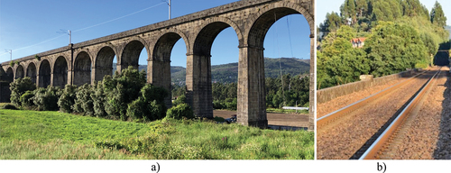
The Durrães bridge, illustrated in Figure 1a, is a multi-span stone arch bridge built in 1878. The bridge extends over 178 m, with 5.3 m width and a maximum height of 22 m from the deck to the ground. It consists of 16 arches, each one with 9 m span, supported by 15 piers and two abutments. The bridge deck (Figure 1b) carries a single electrified railway track on Iberian gauge, with UIC60 type rails and bi-block concrete sleepers laid on a granite ballast layer. On the bridge, it is allowed the circulation of freight and passenger trains with maximum speeds of 100 km/h and 120 km/h, respectively. The bridge is located in northern Portugal as part of Minho railway line which connects Porto to the Spanish border (posteriorly connecting to the region of Galicia). More recently, a daily freight train started to operate on the Minho line transporting timber logs between the Spain production centres and Portuguese pulp factories.

Figure 1. Durrães railway bridge: a) overview; b) railway track.

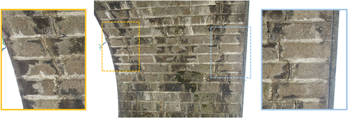
In general, the bridge is in a good condition considering its age (over 100 years old), with minor anomalies associated with the ageing processes of materials. However, there is one relevant structural damage observed in some arches consisting of the existence of longitudinal crack patterns with visible opening of joints. This longitudinal cracking follows the interface between the stones in the first and second row of the arches’ intrados. This is predictably associated with an excessive concentration of stresses due to the traffic loads derived from the increasing traffic. Figure 2 shows a view from the intrados of arch A15, where this damage is visible, with opening joints in the longitudinal direction essentially in the first row of the arch barrel.

Figure 2. Durrães railway bridge: details of the longitudinal cracks on the intrados of arch A15.

2.2. Experimental testing

An extensive experimental campaign was performed in Durrães bridge, comprising both material testing and dedicated structural tests.

The material testing consisted of laboratory tests, for mechanical characterization of the stone and masonry joints, in-situ tests based on Ménard pressuremeter tests, for the characterization of the infill materials, and single/double flat-jack tests for the characterization of the masonry components. The main results of these material testing are available in Arêde et al [49]. In turn, the structural tests involved an ambient vibration test for modal identification [14], as well as dynamic and static tests under freight trains for the characterization of the structural responses in terms of displacements, accelerations and stresses. This section gives an overview of both types of structural testing and the corresponding main results.

2.2.1. Ambient vibration tests

The ambient vibration tests aimed at the estimation of the modal parameters of the bridge, namely, the natural frequencies, mode shapes and damping coefficients. Two dedicated tests were performed, one envisaging the identification of global modal parameters of the bridge, mainly in the transversal and longitudinal directions (Figure 3a), and another focused on the identification of the coupled vertical-longitudinal modal parameters of the central spans of the bridge (Figure 3b).

Figure 3. Experimental setups of the ambient vibration tests: a) global test; b) local test.

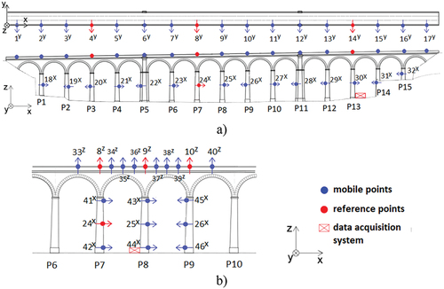
The dynamic tests were performed based on a technique that considers fixed reference points (marked in red colour) and mobile measuring points (marked in blue colour). The ambient vibration response was evaluated in terms of the accelerations in the longitudinal (X) transverse (y) and vertical (z) directions. Six sensor arrangement layouts were used, four in the global test and two in the local test, totalizing 46 measurement points: 25 located on the deck and 21 on the piers.

The tests were performed using 16 uniaxial piezoelectric accelerometers, model 393B12 from PCB, whose main characteristics are presented in Table 1. The table also shows the characteristics of model 393A03, which will be used later. The accelerometers were connected to the side stone guards of the deck as well as to the piers by steel plates glued or bolted to the stone surface. Data acquisition was performed using a cDAQ-9172 system from NI (National Instruments) equipped with 24-bit resolution IEPE type analogue input modules (NI 9234). The time series have been acquired during periods of 10 min, with a sampling frequency of 2048 Hz, posteriorly decimated to 256 Hz.

Table 1. Technical specifications of the accelerometers.

Model	PCB ICP/393B12	PCB ICP/393A03
Resolution (μg)	8	10
Sensitivity (mV/g)	10000	1000
Measurement range (g)	±0.5	±5
Frequency range (Hz)	0.15-1k	0.5–2k
Dimensions (mm)	30.2x55.6	30.2x55.6

The modal identification was performed using the ARTeMIS software based on the Enhanced Frequency Domain Decomposition (EFDD) method [50]. Figure 4 presents the curves of the average normalized singular values of the spectral density matrices. This allowed identifying 11 natural frequencies and corresponding modal configurations of the bridge accordingly to the peaks identified in the figure.

Figure 4. Ambient vibration test: average normalized singular values of the spectral density matrices of all test setups.

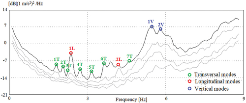
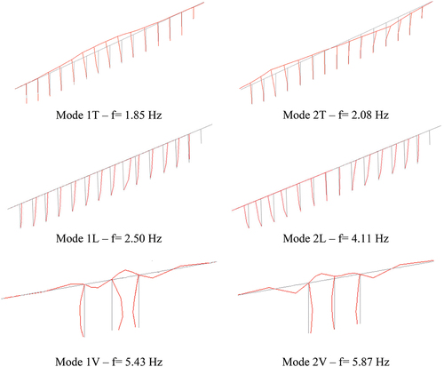
A summary of the modal parameters identified on both global and local ambient vibration tests are presented in Table 2, with an indication of the type of mode shape as well as the natural frequencies and damping coefficient values. The analysis of the modal configurations allows identifying bending movements of the deck and piers in transverse (1T to 7T) and longitudinal (1 L and 2 L) directions and two vertical modes (1 V and 2 V). The average values of the damping coefficients are between 1.34% and 3.61%.

Table 2. Experimental frequencies and damping coefficients identified for Durrães bridge.

Order	Type of mode	Frequency (Hz)	Damping coefficient (%)	Test
1T	Transverse	1.85	2.83	Global
2T	Transverse	2.08	2.43
3T	Transverse	2.41	2.40
1L	Longitudinal	2.50	3.61
4T	Transverse	2.79	3.37
5T	Transverse	3.31	2.51
6T	Transverse	3.83	1.81
2L	Longitudinal	4.11	2.36
7T	Transverse	4.33	1.34
1V	Vertical	5.43	1.67	Local
2V	Vertical	5.87	1.34

In Figure 5 are illustrated, in perspective, the modal configurations of some modes of vibration, particularly the first and second transversal modes, as well as the two first longitudinal and vertical modes. The vertical modes of the bridge’s central arches involve anti-symmetrical (mode 1 V) and symmetrical (mode 2 V) bending movements of the deck as well as the bending of the piers due to structural compatibility.

Figure 5. Experimental modal configurations.

2.2.2. Static loading tests

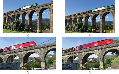
Static load tests aimed at evaluating the bridge response, in terms of deformations and stresses on the piers and arches, under in-service freight trains at specific positions. The instrumented piers and arches were P11/P14 and A11/A15 (see Figure 3), respectively, and the static loading was performed using similar freight trains on two consecutive days. Thus, for Test 1 performed under the first-day train, the instrumentation was installed in arch A11 and pier P11, while for Test 2, referring to the second-day train, the transducers were in arch A15 and pier P14. The transducer layout adopted for Test 1 was repeated for Test 2. The freight train belongs to Takargo, a Portuguese private freight company, and comprises a diesel locomotive Euro 4000 which pulls 14 freight Sgnss type waggons (more details in section 3.2). The instrumentation layout used in the arches and piers is presented in Figure 6.

Figure 6. Static load tests: experimental setup.

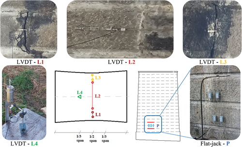
In the arches were installed a set of four Linear Variable Differential Transformers (LVDTs) from RDP (model DCTH) with a measurement range between 5 mm and 15 mm. One LVDT (L4) was used to monitor the vertical displacements at 1/3 span, and the other three (L1, L2 and L3) were strategically positioned at 1/2 span to monitor the opening/closure deformations at different joints located in the arch intrados. Additionally, the stresses in the piers were directly evaluated based on flat-jacks (P) installed at the lower part of the piers in the same positions of previous experimental campaigns performed on the bridge [49]. The flat-jacks were inserted in pre-existing cuts on piers P11 and P14 and a constant pressure was applied to the masonry.

In Test 1, the train entered the bridge at very reduced speed and performed two momentary stops, as illustrated in Figure 7a,b: the first stop (position 1.1) with the front bogie of the locomotive type Euro 4000 over the mid-span of arch A10 (Figure 7a) and the second stop (position 1.2) with the front bogie of the locomotive over the mid-span of arch A11, having its rear bogie over the mid-span of arch A10 (Figure 7b). For Test 2, the train entered the bridge at a very reduced speed, and similarly to Test 1 performed momentary stops as illustrated in Figure 7c,d: the first stop (position 2.1) with the front bogie of a locomotive of the same type over the 1/3 span of arch A15 and the rear bogie over the pier P14 (Figure 7c), and a second stop (position 2.2) with the front bogie of the locomotive over the 1/3 span of arch A16 (Figure 7d).

Figure 7. Static load tests: a) position 1.1; b) position 1.2; c) position 2.1; d) position 2.2.

2.2.3. Dynamic tests under railway traffic

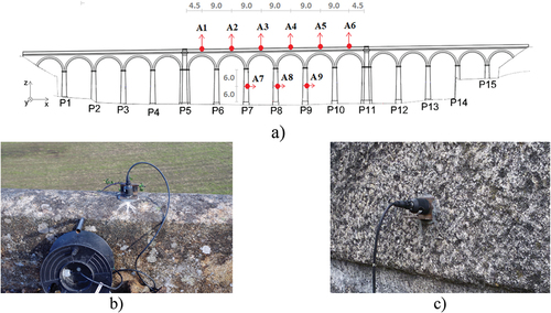
The dynamic test involved measuring vertical accelerations in the arches, as well as longitudinal accelerations in the piers, during the passage of an in-service Takargo freight train (formed by 1 locomotive Euro 4000 and 14 Sgnss waggons). The accelerations were measured in six points on the arches (at the deck level) and three points on the central piers (approximately at half-height), as shown in Figure 8. Uniaxial piezoelectric accelerometers were used, PCB model 393A03 (see Table 1), with a sensitivity of 1 V/g and a measurement range of ±5 g, attending to the higher acceleration levels expected under traffic actions.

Figure 8. Dynamic test: a) setup measurement points in arches and piers (distances in meters); b) accelerometer on the deck; c) accelerometer on the pier.

3. FE numerical models

3.1. Bridge

In a previous work (Costa et al [14]) a global 3D FE model of Durrães bridge was developed and calibrated using modal parameters estimated from the global ambient vibration test. This work contributes to this model improvement at a local level, particularly in the region of arch A15 where longitudinal cracks in arch intrados were identified through visual inspections. This localized damage involves the use of dedicated contact FE elements with adjusted constitutive models to simulate the non-linear behaviour of the discrete cracks within the continuous homogeneous model. Furthermore, the non-linear simulation of the bridge global behaviour is made using a Drucker-Prager model.

Thus, in the first stage, the global modelling and calibration strategy is addressed, and posteriorly, in the second stage, the local modelling and verification strategy is detailed as the main contribution of this work.

3.1.1. Global modelling and calibration

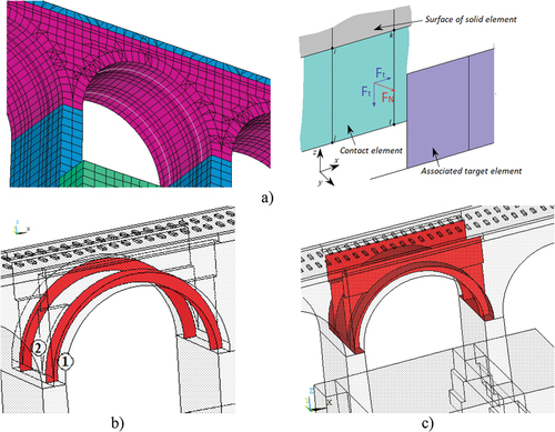
The global numerical modelling of Durrães bridge was performed using a 3D FE model developed in ANSYS® software [51]. Figure 9 shows the numerical model of the bridge with the identification of several structural components. The arches, piers, spandrel walls, backfill, abutments, foundations, embankment, rails, ballast and sleepers, were modelled using volumetric finite elements of hexahedral and parallelepiped shape with 6 and 8 nodes, respectively. The side guards were modelled through mass elements distributed over both spandrel walls. The boundary conditions were established using rigid supports fixing all displacements of the nodes of the finite element mesh located at the base of the foundations and abutments. The complete model of Durrães bridge consists of 88,908 FE elements and 105,306 nodes. The mean element size is 0.40, while the maximum and minimum element dimensions are equal to 0.96 m and 0.09 m, respectively.

Figure 9. 3D global numerical model of Durrães bridge [39].

The global calibration of the FE model of the bridge relied on modal parameters, particularly natural frequencies and mode shapes, and involved the application of an iterative methodology based on an optimization process. The optimization involved the use of a genetic algorithm envisaging the minimization of the residuals of an objective function that includes the residuals of the natural frequencies and modal configurations. From the calibration, the optimal values of 8 material parameters were obtained, particularly the correction factors of the elastic modulus of the masonry elements, including the arches, spandrel walls, piers and abutments, located in different areas of the bridge.

Some other parameters related to specific material properties of the masonry and infill of the bridge were directly defined based on the results of laboratory and in-situ tests according to the details presented in Costa et al [14]. These parameters were not included in the calibration process and considered as deterministic.

The elastic material properties of the masonry (in the bridge zones of foundations, piers, arches and spandrel walls) and infill are characterized by the elastic modulus, Poisson’s ratio and unit weight listed in Table 3. The elastic characteristics of the ballast, sleepers, embankments and rails are also summarized in Table 3.

Table 3. Elastic and mass parameters of the FE model of Durrães bridge.

Parameter	Material	Adopted value	Unit
Elastic modulus	Masonry of arches, spandrel walls, piers and abutments (*)	6.6–10.7	GPa
	Masonry of foundations	15
	Infill (upper/lower) (**)	0.6/1.0
	Embankments	0.75
	Ballast	0.15
	Sleepers	36.0
	Rail	210.0
Unit weight	Masonry	24.5	kN/m^3
	Infill	21.5
	Embankments	20.0
	Ballast	20.0
	Sleepers	28.9
	Rail	78.5
Poisson’s ratio	All	0.2	-

*Optimal values obtained through optimization.

**Estimated values based on in-situ experimental tests.

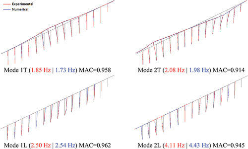
After the calibration process, the average error of the natural frequencies associated to global modes, taking as reference the corresponding experimental values, was equal to 4.0% and the average MAC value equal to 0.926. Figure 10 shows the comparison between the experimental and numerical configurations of two transversal (1T and 2T) and longitudinal (1 L and 2 L) mode shapes (according to Figure 4). In the figure, is also indicated in brackets, the values of the experimental (in red) and numerical (in blue) natural frequencies, as well as the corresponding MAC values.

Figure 10. Comparison between some of the numerical and experimental global modal parameters of Durrães bridge.

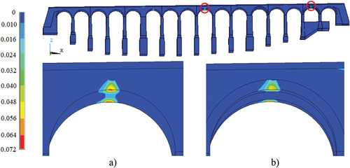
3.1.2. Local modelling and verification

The local modelling strategy involves a refinement of the global FE model in the region of arch A15 where longitudinal cracks were observed on both sides of the arch intrados (see Figure 2b). The damage simulation involves the use of contact FE elements to simulate the non-linear behaviour of the joints between the masonry blocks, following the methodology presented in [52]. Thus, a surface-to-surface contact model including friction and cohesive behaviours is used for the block-to-block interfaces of arch A15. Figure 11a schematically represents the layout of a surface-to-surface contact model in ANSYS®.

Figure 11. 3D local numerical model of Durrães bridge: a) arch A15 and adopted contact model; b) location of contact/target elements on both spandrel walls interfaces; c) location of contact/target elements on other interfaces.

The interaction between the two surfaces in contact is controlled by the forces they exert on each other, and how the forces are transferred in both normal and tangential directions at the points of contact [53]. The force vector can be resolved into normal and tangential components F_N and F_T, dependent of a normal contact stiffness, K_n, and a friction contact stiffness, K_s, respectively. The normal component prevents the surfaces from penetrating into each other, as the tangential component prevents from sliding over each other.

Pairs of contact/target elements (CONTA173/TARGE170) with 4 nodes were included in specific locations of the FE model and merged to the surfaces of the masonry solid elements of the arch A15. Thus, two sets of contact/target FE elements with different contact properties were defined:

1. on both spandrel walls’ interfaces, where the longitudinal cracks were observed (Figure 11b). In this case, the contact/target elements, as well as the masonry solid elements, were positioned in a straight alignment which approximately follows the real crack path, with a depth of 0.6 m (identified by 1 and 2).

2. on other interfaces, namely, the interfaces between arch and infill, spandrel walls and infill, and arch with piers (Figure 11c). For these interfaces no experimental results are available.

The two simulated longitudinal cracks shown in Figure 11b represents longitudinal cracks that are already open and with a zero tensile strength, whose opening resistance is only controlled by the bed joints with shear strength. In these bed joints, the shear strength is characterized for exhibiting only residual shear behaviour. Therefore, the assumed straight alignment for the longitudinal cracks represents the shear behaviour (controlled by K_s) by means of a normal stress behaviour joint, with tensile strength (controlled by K_n). Thus, a frictional contact was established at the interface by assigning in the normal direction a stiffness K_n in compression and no tension stiffness, as well as a shear stiffness K_s in the tangential direction. For this contact formulation, the Penalty function algorithm was adopted [53].

Figure 12a presents the normal contact model behaviour. The normal stress–displacement curve (σ-δ) shows a linear elastic loading associated with a constant normal stiffness (K_n) followed by a linear softening branch (represented in red in Figure 15a) where the tensile stress decrease from its maximum value (σ_max) until zero. The tension behaviour is reproduced by adopting a Cohesive Zone Model (CZM), available in ANSYS® and proposed by Alfano and Crisfield [54]. When under compression the recontact of the two surfaces is always possible defined by the normal stiffness parameter.

Figure 12. Contact model behaviour: a) normal direction; b) tangential direction.

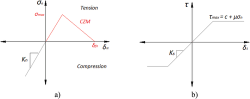
Figure 12b presents the tangential contact model, in this case, a Coulomb friction model, which is characterized by a proportionality between frictional (τ) and normal (σ) forces. The two surfaces have a specific friction coefficient and null cohesion (c). The slippage occurs when the critical load value (τ_max) is reached.

Normal and friction stiffness contact parameters were derived from the values estimated from shear tests conducted in joint samples extracted from the bridge, as detailed by Arêde et al [49]. These tests allowed to estimate the shear response using split joint samples and considering three different normal stress levels. The results showed two phases, a quasi-linear elastic phase until reaching the maximum shear stress values, followed by a residual strength phase.

For the contact/target elements simulating the longitudinal cracks in the arch, a normal-stress stiffness value (K_n) of 0.60 MPa/mm and 0.40 MPa/mm was adopted, respectively for alignments 1 and 2 (see Figure 11), and a shear-stress stiffness value (K_s) equal to 10 MPa/mm. For the other interfaces, a higher value of normal stiffness was considered to prevent excessive deformation. Table 4 lists the main contact parameters assigned to all the contact/target FE elements.

Table 4. Contact elements’ parameters.

Contact/target interface	Kn (MPa/mm)	Ks (MPa/mm)	Coefficient of friction
Arch and Infill	6	10	0.75
Spandrel and Infill
Arch and Piers
Crack - alignment 1	0.4
Crack - alignment 2	0.6

The non-linear material behaviour of the masonry (arches, spandrel walls and piers) and infill was reproduced by the Drucker-Prager model available in ANSYS software [51] and presented in Figure 13.

Figure 13. Material model behaviour: a) exponential hardening and softening in compression; b) exponential softening in tension.

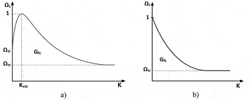
Drucker-Prager model requires the definition of the uniaxial and biaxial compressive strengths, f_c and f_cb respectively, and the tensile strength f_t, as input material properties. An associated flow rule was followed by defining the dilatancy factor, ∆, equals to 1. The definition of these values was based on the experimental characterization of masonry and infill materials detailed in Arêde et al [49]. In the compression domain, an exponential hardening/softening function (Figure 13a) was adopted based on the following parameters: plastic strain at uniaxial compressive strength, K_cm; relative stress at onset of hardening, Ω_ci; residual compressive relative stress, Ω_cr; and Mode I specific fracture energy in compression, G_fc. In the tension domain, an exponential softening function (Figure 13b) was adopted based on the following parameters: residual tensile relative stress, Ω_tr and Mode I specific fracture energy in tension, G_ft .

All the input parameter values required for both compression and tension models are presented in Table 5. These values were derived from a numerical simulation of the double flat-jack tests performed on the bridge [49], using the methodology presented in Costa et al [55]. based on non-linear FE modelling.

Table 5. Drucker-Prager (D-P) model parameters.

D-P input parameters		Hardening/softening model
Parameter	Value/Unit	Parameter	Value/Unit
ft	0.1 MPa	∆	1.0
fc	4.0 MPa	Kcm	3.9 ‰
fcb	4.8 MPa	Ωci	0.30
		Ωcr	0.30
		Gfc	16 N/mm
		Ωtr	0.1
		Gft	0.025 N/mm

The local model verification was based on the comparison between the experimental and numerical modal parameters for two identified local vertical modes (Figure 14). This comparison is performed considering the longitudinally cracked model of Durrães bridge presented in Figure 11. As can be stated by the figure, there is a very good correlation between experimental and numerical results. In particular, the frequencies relative errors are equal to 2.7% and 4.9%, and the MAC values are 0.891 and 0.904, for modes 1 V and 2 V respectively. In the Figure 14 were also included the frequencies values derived from the numerical model without longitudinal cracks (marked with asterisk). As can be stated the differences between the frequencies values obtained with the non-cracked and cracked models are very small.

Figure 14. Comparison between the numerical and experimental local vertical modal parameters of Durrães bridge.

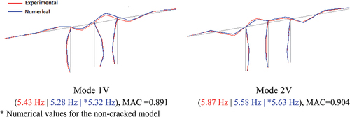
* Numerical values for the non-cracked model

3.2. Train

The freight train used in the experimental testing of Durrães bridge, summarily described in section 2, is composed of a diesel locomotive Euro 4000 and 14 freight waggons Sgnss series loaded with timber logs (Figure 15a). Figure 15b shows a schematic representation of the locomotive and waggons with information about axle loads and axle spacings. The locomotive has 6 axles with an average axle load of 204 kN, and the Sgnss waggon has 4 axles and an average axle load of 202 kN. In normal operation, each waggon is considered to have an average mass of timber logs equal to 82 t and a tare load of 26.5 t, totalizing 202 kN per axle. The mass of timber logs was estimated based on weighting data obtained during the waggons unloading at Navigator pulp industry.

Figure 15. Takargo freight train: a) general view; b) loading scheme (dimensions in metres and static loads in kN); c) train dynamic signature.

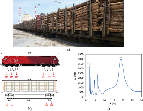
Figure 15c shows the dynamic signature (S₀) of the train considering wavelengths between 1 m and 30 m. The dynamic signature of a train is a reference parameter for representing the parametric dynamic excitation induced by the train, which depends on the values of axle loads and distance between axles, and can be obtained by [56]:

(1) $S_0\left(\lambda \right)=\underset{i=1,N}{max}\sqrt{{\left[\sum _{k=0}^i{P}_{k}cos\left(\frac{2\pi x_k}{\lambda }\right)\right]}^2+{\left[\sum _{k=0}^i{P}_{k}sin\left(\frac{2\pi x_k}{\lambda }\right)\right]}^2}$(1)

where $\lambda$ represents the wavelength, P_k is the load value of the k axle, x_k is the distance of the k axle to the first axle of the train and N is the number of axles of the train. The peaks identified in Figure 15c correspond to the wavelengths for which the train is more aggressive and, consequently, more prone to excite the railway bridge. Particularly, the wavelength of 19 m is related to the distance between groups of two consecutive axles belonging to different waggons. Also, the wavelength of 1.8 m represents the axle distance. The identified wavelengths may not correspond to the exact distances between the train axle groups due to perturbations caused by nearby wavelengths from the locomotive or other characteristic distances of the waggons.

In a previous work, Silva et al [48], developed a 3D FE model of the Sgnss waggon in ANSYS® software (Figure 16a). This model was calibrated based on modal parameters derived from a dynamic test and considering two distinct static loading configurations, tare weight and current operational overload [48].

Figure 16. Freight train FE model: a) Sgnss waggon, b) bogie detail.

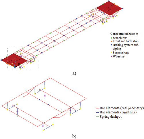
The waggon’s main platform, bogie frames and axles were modelled with beam finite elements (BEAM 188), considering their corresponding geometrical properties. The plates attached to the platform extremities were modelled through shell elements (SHELL 181) considering their real thickness. The bogie frames and axles were modelled using flexible beam elements, based on their corresponding geometrical properties, and the axle boxes and spring holders were modelled using rigid beam elements. The suspensions were modelled as spring-dashpot assemblies using COMBIN14 elements in the vertical direction. The wheel-rail contact is modelled by a spring-dashpot assembly in the vertical direction (COMBIN14) whose stiffness is estimated from the Hertz contact theory [57].

The vehicle tare mass was incorporated into the model by an equivalent density of the steel girders and plates, however, concentrated mass elements (MASS21) were added to consider the mass of specific non-structural elements, namely the stanchions, suspensions and other bogie components. The positioning of the concentrated masses is presented in Figure 16, where a detail of one bogie is also shown.

The calibration of the waggon FE model relied on modal parameters, particularly natural frequencies and mode shapes, and involved the application of an iterative methodology based on a genetic algorithm. From the calibration, optimal values of 8 numerical parameters were estimated, namely, the side bearers’ vertical stiffness, the stanchion masses, the vertical stiffness of the primary suspensions, the steel deformability modulus and the masses of the back and front metallic plates. Table 6 presents the geometrical and mechanical characteristics of the main elements of the loaded Sgnss waggon, with the identification of the parameters obtained through the optimization process.

Table 6. Main parameters of the numerical model of Sgnss vehicle (loaded configuration).

Parameter	Value	Unit
Steel properties
Deformability Modulus	215*	GPa
Density	8.0	g/cm^3
Masses
Mass of metallic plates (per node)	320*	kg
Mass of stanchion (per node)	100*	kg
Mass of braking system and piping	150	kg
Mass of wheelset	1112	kg
Mass of suspensions components	220	kg
Primary Suspension
Vertical stiffness Spring set 1 Spring set 2 Spring set 3 Spring set 4	6600* 6600* 6000* 6000*	kN/m
Side bearers vertical stiffness	1650*	kN/m
Damping	19	kN.s/m
Secondary Suspension
Stiffness	1x10^9	kN/m
Hertzian spring wheel-rail	1.53x10^7	kN/m

*Optimal values obtained through optimization.

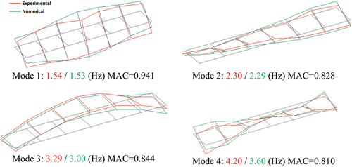
Figure 17 shows the comparison between some experimental and numerical modal parameters of the loaded Sgnss waggon. The results show a good correlation between the experimental (in red) and numerical (in green) modal configurations, with an average error of natural frequencies equal to 4.8% and an average MAC value of 0.851.

Figure 17. Comparison between some of the numerical and experimental modal parameters of Sgnss wagon (loaded configuration).

The calibrated waggon model on loaded configuration will be considered for the train-bridge dynamic interaction analysis of Durrães bridge (Sections 4 and 5). The locomotive is simply introduced into the dynamic problem as a set of constant moving loads according to the respective axle positions.

3.3. Train–bridge interaction

The numerical analysis of the train-bridge system was based on a dynamic analysis considering vehicle – structure interaction and including the measured track irregularities.

The vehicle – bridge dynamic interaction was implemented in ANSYS® software based on a dedicated contact approach. The dynamic interaction only considers the vertical direction and allows the sliding and loss of contact at the wheel–rail interface. The vertical wheel-rail contact deformability was simulated based on a Hertzian spring (Table 6). Figure 18a presents an overview of the vehicle – structure dynamic interaction model.

Figure 18. Train–bridge interaction model: a) overview; b) detail of the wheel-rail contact and c) contact/target pair scheme.

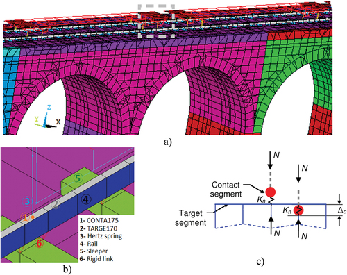
The dynamic analysis of the vehicle-bridge system is performed considering both subsystems, train and bridge, modelled as a coupled system using advanced contact finite elements at the wheel–rail interface. In particular, the wheel–rail interaction was modelled using a node-to-surface contact algorithm, defining as contact point (CONTA175) the end of the wheel-rail spring element, and as target surface (TARGE170) the top of the rail profile defined by solid finite elements. The connection between rails and sleepers was performed through rigid links. The flexibility provided by the rail pads, and corresponding filtering effect, was neglected. The inclusion of this flexibility would be relevant to properly evaluate the dynamic response on the track components, however, have typically a negligible effect on the global dynamic responses of the bridge [3]. The geometry of the rail was simplified to a rectangle with area and inertia equal to the original UIC60 type. This simplified approach is feasible since this study is focused only on the vertical wheel-rail dynamic interaction, and therefore the lateral and longitudinal interactions are not considered.

Figure 18b shows a detail of the wheel-rail contact and Figure 18c the contact/target pair formulation. For the wheel–rail interaction, the Penalty algorithm was adopted [53] and the full Newton – Raphson method [58] was used to solve the non-linear equations of the problem. Some key options of the pair-based contact model are presented in Table 7.

Table 7. Key options set for the contact-pair model [51].

Key option (number)	Adopted setting
Contact algorithm (2)	Penalty function
Adjusting initial conditions (ICONT) (5)	Auto ICONT
Effect of initial penetration or gap (9)	Exclude both
Contact Stiffness Update (10)	Update each iteration
Behaviour of contact surface (12)	No separation

According to the contact formulation schematized in Figure 18c, the normal contact force appears when there is a certain penetration, Δc, of the contact element into the target element. The normal force, N, is proportional to Δc, and the constant of proportionality is the normal stiffness parameter, K_n. Dynamic systems are very sensitive to K_n, so a high value of K_n would produce high impact forces and accelerations; otherwise, a low value of K_n would produce smaller forces and large penetrations [59]. In order to achieve contact compatibility and convergence, a value of K_n equal to 1.0 × 10⁸ kN/m was adopted.

An additional track extension was modelled before and after the bridge, to provide continuous support for the train model during the dynamic analysis. The movement of the vehicle over the rails was defined by a prescribed speed in the x-direction to all nodes of the train model, which makes the contact element move together [60]. Vertical static loads were applied to all the contact nodes.

3.4. Track irregularities

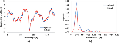
The track irregularities were obtained based on records provided by EM120 track inspection vehicle from the Portuguese railway infrastructure manager. Figure 19a illustrates the longitudinal levelling profiles of the left and right rail over Durrães bridge. These records consider the contributions related to wavelengths between 3 m and 70 m spaced from 0.25 m. The longitudinal levelling values are inside 6 mm in amplitude, except for the central part of the bridge where they reach a value close to 10 mm. Figure 19b shows the auto-spectra amplitude for the irregularities on both rails, as a function of the wavenumber (1/λ). The highest amplitudes are registered for wavelengths values between 40 m and 50 m, and with a less pronounced peak in the interval between 14 m and 17 m. The irregularity profiles were directly modelled on the rail finite elements by a detailed geometric adjustment at each 0.25 m spacing.

Figure 19. Irregularities profile on Durrães bridge: a) longitudinal levelling b) auto-spectra amplitude.

4. Validation

The validation of the non-linear FE numerical model of Durrães bridge (section 3.1) involves a two-step strategy. First, the results derived from a numerical static analysis under the locomotive Euro 4000, at two specific positions, are compared with the corresponding responses obtained from the static loading tests. Second, a numerical dynamic analysis of the train-bridge system is performed for the passage of Takargo train and the corresponding responses are compared with the ones obtained from the dynamic tests under railway traffic.

4.1. Static analysis

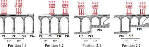
The numerical static analysis was performed considering four different positions of the locomotive Euro 4000, according to the loading schemes detailed in Figure 24, which simulate the experimental configurations. In this figure, the isolated forces (in red) represent the axle loads of each bogie of the locomotive Euro 4000. To simulate the load test 1, two positions were considered, positions 1.1 and 1.2, while for load test 2, two additional positions were defined, in this case positions 2.1 and 2.2.

Figure 21 shows the values of the experimental and numerical vertical displacements evaluated with the LVDTs installed at 1/3 span of arches A11 and A15, for loading tests 1 and 2, respectively, in correspondence to the positions of Figure 20. For these positions, the graphs allow reading the corresponding static displacement values.

Figure 20. Loading cases for the static numerical analysis.

The experimental results plotted in Figure 21a referred to arch A11 show that for position 1.1 the load applied in arch A10 causes an upward movement on arch A11 around 0.10 mm. This result is consistent with the influence line relative to the vertical displacement at 1/3 span of arch A11, for which a descending load applied in arch A10 causes an opposite direction deflection in arch A11. When the train moves to position 1.2, with the first bogie of the locomotive passing over the 1/3 span of arch A11, the maximum downward deflection reaches around 0.45 mm and then reduces to 0.30 mm when the train stops at the established position. For arch A15, the graph in Figure 21b shows that the experimental maximum downward displacement is around 0.60 mm and occurs for the train in position 2.1. For position 2.2, the maximum upward vertical displacement measured in arch A15 is around 0.15 mm. Again, considering the influence line for the vertical deflection at 1/3 span of arch A15, the load applied in adjacent arches has an opposing effect in the response measured in arch A15.

Figure 21. Experimental vs Numerical static vertical displacements: a) load test 1 (positions 1.1 and 1.2); b) load test 2 (positions 2.1 and 2.2).

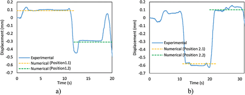
For both tests, a very good agreement was found between numerical and experimental vertical displacements. In particular, the numerical vertical displacement at 1/3 span of arch A11 for position 1.1 was equal to +0.09 mm and for position 1.2 equal to −0.30 mm. In the case of load test 2, the vertical displacement at 1/3 span of arch A15 for position 2.1 was equal to −0.58 mm and for position 1.2 equal to +0.10 mm.

The vertical stress records measured by the flat-jacks installed on piers P11 and P14 are presented in Figure 22a,b, respectively. The results evidence that the relative variations of vertical stresses in the masonry piers are in accordance with the train axles’ movements shown in Figure 21a,b. For pier P11, a minimum vertical stress release of approximately −20 kPa is observed, which is consistent with the corresponding upward displacement of arch A11 in position 1.1. Afterwards, the maximum vertical stress increases to 29 kPa (close to 20s) corresponding to the passage of the front bogie of the locomotive over pier P11. For pier P14, the maximum vertical stress occurs when the front bogie of the locomotive passes over P14, is around 28 kPa and is in accordance with position 2.1.

Figure 22. Stress variation on the bridge piers under permanent and live loads for pier P11 and P14: a) and b) experimental results; c) and d) numerical results.

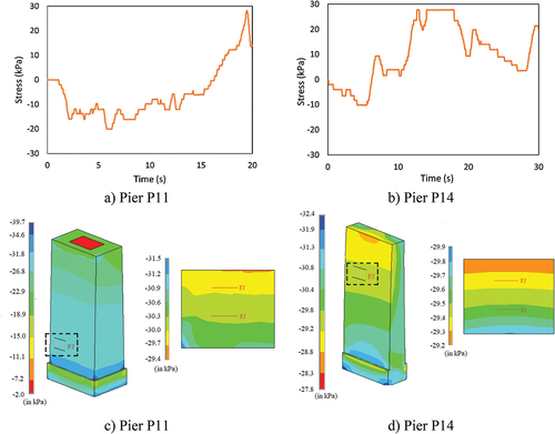
Figure 22c,d shows the variation of the vertical compressive stresses, evaluated numerically, in the piers P11 and P14, due to the locomotive loading. For each case, the results due to the live loads are presented. Also, the exact locations in both piers where the flat-jack tests were performed are identified by ‘FJ.’ The numerical responses on both piers are in good agreement with the flat-jack test results of Figure 22a,b. For pier P11, shown in Figure 22c an average stress variation of 30 kPa was estimated under the same loading conditions. For pier P14, shown in Figure 26c a maximum stress variation of around 29.5 kPa is measured for the loading scheme corresponding to the locomotive front bogie positioned over the pier.

The values of compressive stresses due to permanent loads are equal to 577 kPa and 614 kPa for piers P11 and P14, respectively. This finding proves that the vertical stress variation values due to the passage of the locomotive are approximately 5% of the values registered for permanent loads on both masonry piers.

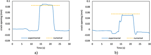
Figure 23 presents the relative displacements in the longitudinal cracks located on the spandrel wall interfaces of arch A15 measured by the LVDTs L1 to L3, respectively. Specifically, a comparison is performed between the values obtained from the numerical analysis and the experimental tests. The magnitudes of these opening movements are quite small for the monitored arch portions based on L1 and L3 transducers. For the contact interface located on the side of transducer L1, the maximum value of crack opening equals 0.06 mm, and on the side of transducer L3, a maximum value of 0.08 mm is achieved. As stated by the figures, these numerical values are in very good agreement with the displacements measured on the experimental tests.

Figure 23. Experimental and numerical crack opening values on the spandrel wall interfaces of arch A15: a) on the side of transducer L1; b) on the side of transducer L3.

4.2. Dynamic analysis

The non-linear dynamic analysis considered the train-track-bridge interaction and the measured irregularities profiles. The Rayleigh damping coefficients for the bridge (α = 0.208 and β = 0.002) were estimated setting the damping coefficients equal to 2% for the 1st and the 10th vibration modes of the bridge. These two modes correspond to the first transversal and vertical modes, respectively. The time step considered in the analyses was equal to 0.01 s.

Figure 24 shows a comparison of the experimental and numerical vertical acceleration time series in the locations A2 and A5 of the bridge deck (according to Figure 8a) for the passage of the freight train at 60 km/h. The power spectrum density (PSD) function of the acceleration records is also presented, as well as the dynamic signature of the train as a function of the frequency of excitation. Figure 25 presents similar information but considers the experimental and numerical longitudinal acceleration time series in locations A8 and A9 at half-height of the bridge piers (according to Figure 8a). The experimental time series were filtered using a Butterworth low-pass digital filter with a 30 Hz cut-off frequency and filter order of 5. The maximum vertical accelerations experimentally recorded on the deck occurred during the passage of the locomotive, with peak values around 0.30 m/s². Concerning the piers, the maximum longitudinal accelerations recorded were considerably lower than those measured on the deck and approximately equal to 0.10 m/s².

Figure 24. Dynamic responses for the passage of the freight train at 60 km/h at mid-span of the arches in the vertical direction: a) accelerations time series, b) PSD amplitude, c) train dynamic signature.

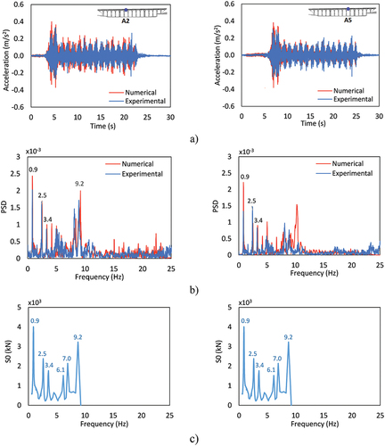
Figure 25. Dynamic responses for the passage of the freight train at 60 km/h at half-height of piers in the longitudinal direction: a) acceleration time series, b) PSD amplitude, c) train dynamic signature.

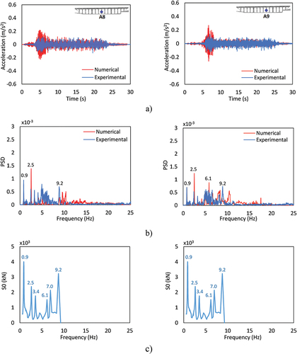
The vertical acceleration records presented in Figures 24a and 25a show a good agreement between numerical and experimental responses, particularly concerning the parts of the records related to the passage of the waggons. For these parts of the records, the breathing effect induced by the passage of regularly spaced groups of axles is quite well reproduced, as well as the peak acceleration values. For the initial parts of the records, related to the passage of the locomotive, the peak acceleration values obtained from the numerical simulation are higher in comparison to those derived from the experimental measurements. These differences are probably related to the fact the locomotive was simply simulated as a set of moving loads, due to the inexistence of information from the manufacturer. The consideration of a locomotive-bridge interaction would allow an energy transfer between these two subsystems, which would predictably reduce the bridge response, guaranteeing a better convergence between experimental and numerical results.

Comparing the PSD plots of Figures 24b and 25b, a good agreement is found in terms of amplitude peaks between the experimental and numerical dynamic responses. Most of the main peaks are directly justified by the influence of the parametric excitation of the train action. For a speed of 60 km/h the frequency (f) associated with the passage of regularly spaced bogies, λ = 19 m, is equal to 0.9 Hz (f=v/λ), and the frequency associated with the passage of the regularly spaced axles, λ = 1.8 m, is equal to 9.2 Hz. Also, for the frequency of 2.5 Hz, associated with the distance between axles of two consecutive waggons, some dynamic amplification phenomenon is observed, particularly for the longitudinal responses. In fact, this frequency is also related to the natural frequency of the first longitudinal mode of the bridge.

The track irregularities present prominent wavelengths between 10 m and 50 m, and therefore are particularly prone to excite the bridge in the frequencies interval between 1.7 Hz and 0.3 Hz, respectively. At these frequencies range, a good approximation between experimental and numerical results was verified.

Figure 26 shows the state of plasticity of the bridge structural elements in terms of maximum principal plastic strains for the passage of a freight train at 60 km/h. As can be stated, for this service loading the bridge response exhibits non-linear incursions at several arches, particularly at arches A9 and A15. The maximum values of 0.072‰ and 0.056‰ obtained, respectively, for arch A9 and arch A15 are concentrated in the lateral zones of the arches, where occur significant tensile stresses. These identified critical zones are in accordance with the damages observed in the arches’ intrados, where longitudinal cracks were found between the first and second rows of the masonry blocks (see section 2.1). For the infill material, no plastic deformations are observed, as stated in Figure 26.

Figure 26. Plastic strain level in terms of principal maximum strains (in ‰) for the freight train passage at 60km/h: a) arch A9; b) arch A15.

5. Simulation

5.1. Scenarios

The train running speed over the bridge is one of the parameters that most affect the dynamic response of the train-bridge system. Although the maximum circulation speed over Durrães bridge is 100 km/h, in the dynamic study of the bridge it should be predicted the possible future increase of the operating speed for freight trains. Thus, a simulation of the dynamic behaviour of the train-bridge system was performed for speeds between 40 km/h and 140 km/h, with increments of 10 km/h, and considering the track irregularities. This study will allow to identify critical operating speeds that would amplify the dynamic response at specific arches.

5.2. Bridge response

The bridge dynamic response was evaluated based on the maximum values of the vertical displacements and accelerations in specific arches, as a function of the circulation speed. Figure 27 shows the results of the maximum vertical displacements (Figure 27a) and accelerations (Figure 27b) monitored at the mid-span of the arches A1, A2, A8, A9, A11, A15 and A16. The results are presented for the arches located on both extremities of the bridge, as well as in the central region of the bridge, including the arches A11 and A15, which were experimentally tested.

Figure 27. Maximum vertical dynamic response of several arches of Durrães bridge for the passage of the freight train for speeds between 40 km/h and 140 km/h in terms of: a) displacements; b) accelerations.

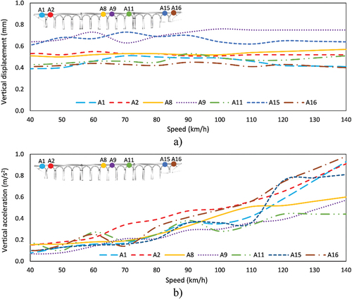
The maximum vertical displacements on the arches show a reduced variation as a function of the circulating speed. The maximum values are obtained for arch A9, located in the central region of bridge, with a value of around 0.7 mm.

The maximum vertical accelerations on the arches are ranging between 0.1 m²/s and 1.0 m²/s for the maximum speed considered. The results show a global tendency of increasing accelerations with the increasing of speeds for all arches. Particularly, for speeds higher than 60 km/h the maximum acceleration levels tend to vary linearly with the speed increase. The arches located in the extremities of the bridge (A1, A2, A15 and A16) are the ones that present higher acceleration values. For the speed of 140 km/h, arch A16 is the one that presents the maximum acceleration value, probably due to the shorter height piers, which conducts to a higher global stiffness. All the acceleration values are within the regulatory limit of 3.5 m²/s for ballasted tracks according to EN 1990-Annexe A2 [61].

Based on the analysis of Figure 27, no resonance speeds, nor speeds eventually responsible for higher amplifications of the dynamic responses, were identified. This may be justified due to the separation between the main natural frequencies of the bridge from the parametric excitation frequencies of the waggons, according to the train dynamic signature. As an example, considering the dynamic signature peaks associated with wavelengths (λ) of 1.8 m and 19 m, and for the extreme speeds (v) of 40 km/h and 140 km/h the mobilized frequencies (f=v/λ) are within the range [6.17–21.6] Hz, for λ = 1.8 m, and [0.58–2.0] Hz, for λ = 19 m. Since the main natural frequencies of the bridge are in the range [1.85–5.87] Hz, the train excitation frequencies are outside this critical interval.

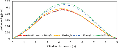
Figure 28 shows the maximum crack opening in the longitudinal crack simulated on arch A15. The results are obtained for five different speeds and measured in the contact elements along the arch span. For the train passage at 60 km/h, the maximum crack opening value is around 0.09 mm, and this value remains approximately the same until a speed of 100 km/h. For the speeds of 120 km/h and 140 km/h, the values significantly increase until reaching a maximum deformation of around 0.11 mm at a speed of 140 km/h.

Figure 28. Crack opening values on the spandrel wall interface of arch A15 due to the freight train passages at 60, 80, 100, 120 and 140 km/h.

5.3. Train response

Figure 29 shows the maximum vertical acceleration of the first, intermediate and last waggons of the freight train, for the speed range between 40 km/h and 140 km/h, and considering the measured track irregularities. Monitoring points are in five positions, namely, at the mid-span and extremities of the waggon platform and in two positions on the bogies.

Figure 29. Maximum vertical accelerations at different points of the waggon’s platform for the: a) first waggon, b) intermediate waggon, c) last waggon.

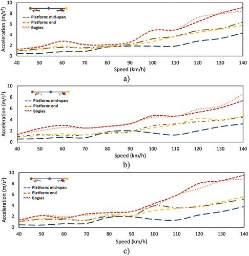
Concerning the platform, the maximum values obtained at the extremities are larger than those evaluated at the mid-span, due to the contribution of the pitching vibrations. Additionally, the results show that the maximum acceleration values evaluated on the waggon’s platform are lower than the values obtained on the bogies. Particularly, the order of magnitude of the accelerations on the waggon’s platform is between 1.0 m/s² and 6.0 m/s², and in the bogies between 1.0 m/s² to 10.0 m/s². This is due to the filtering effect of the secondary suspension system, which is responsible for removing the high-frequency content of the bogies’ acceleration records and consequently reducing the maximum accelerations at the platform’s level. Finally, the acceleration levels on the first, intermediate and last waggons of the freight train remain approximately similar. This is probably due to the high vertical stiffness of the bridge and the reduced amplification levels of displacement during the passage of the successive train waggons.

6. Conclusions

This article described the validation of a FE numerical model of Durrães bridge based on experimental data obtained from static and dynamic tests under freight traffic actions. The train consists of a locomotive Euro 4000 and Sgnss waggons transporting timber logs. The dynamic analysis of the vehicle-bridge system was based on advanced interaction models, including the measured track irregularities. Both, the bridge and the freight waggon FE models were previously calibrated based on dedicated dynamic tests.

An extensive experimental campaign was performed on Durrães bridge, comprising both material testing and dedicated structural tests. The structural tests involved an ambient vibration test for modal identification, as well as static and dynamic tests under freight trains. The static load tests comprised the measurement of vertical displacements in the arches, stresses on the piers and the opening/closure deformations in different joints between masonry blocks of the arches. The magnitudes of these opening movements are reduced, in the order of 0.06 mm to 0.08 mm. For the maximum vertical deflection, values of 0.45 mm and 0.60 mm were measured at 1/3 span of arch A11 and arch A15, respectively. Resorting to a flat-jack test installation in two piers, the relative variations of vertical stresses due to the train axle loading were measured in the masonry, with a maximum value around 30 kPa obtained for both locations. The dynamic tests comprised the measurement of vertical accelerations in the bridge deck, as well as longitudinal accelerations in the piers, for a train passage at 60 km/h. The maximum vertical accelerations recorded on the deck occurred during the passage of the locomotive, with peak values around 0.30 m/s² and for the passage of the regularly spaced axles of the waggons a peak value of 0.20 m/s².

For the bridge numerical model, a non-linear model was adopted using a Drucker-Prager model allowing a softening representation in the tensile domain, which is particularly important for the masonry material. Additionally, the bridge numerical model was improved at a local level, in the case of arch A15, where longitudinal cracks in arch intrados were identified through visual inspections. This localized damage involved the use of dedicated contact FE elements with adjusted constitutive models. The adopted strategy allowed simulating the non-linear behaviour of the discrete cracks within the continuous homogeneous model.

The validation of the non-linear FE model of the bridge involved a two steps strategy. Firstly, the results derived from a numerical static analysis under the locomotive were compared with the corresponding responses obtained from the static loading tests. The numerical values are in very good agreement with the displacements measured on the experimental tests, namely, vertical deflections and opening displacements on the longitudinal cracks. For the compressive stresses, the numerical responses on both piers are in good agreement with the stress variation registered in the flat-jack tests. Secondly, a numerical dynamic analysis of the train-bridge system was implemented in ANSYS® based on a dedicated contact formulation and the numerical responses were compared with the ones obtained from the dynamic tests. The numerical and experimental vertical acceleration records show a good agreement, in terms of peak acceleration values as well as amplitude peaks obtained through PSD plots.

Finally, the dynamic behaviour of the train-bridge system was performed for realistic scenarios of freight traffic comprising speeds between 40 km/h and 140 km/h. A maximum vertical acceleration value of 1 m/s² was obtained on the arches for the freight train passage, which is within the normative limits of EN 1990-Annexe A2. No resonance phenomenon, nor speeds eventually responsible for higher amplifications of the dynamic responses in the arches were identified. Concerning the response in the waggons of the freight train, the results showed that the maximum acceleration values evaluated on the first, intermediate and last waggons remain approximately similar, probably due to the high vertical stiffness of the bridge and reduced amplification levels of the displacement during the successive waggon’s passage.

Acknowledgements

The authors would like to acknowledge the support of the Base Funding UIDB/04708/2020 and Programmatic Funding UIDP/04708/2020 of the CONSTRUCT (Instituto de I&D em Estruturas e Construções) funded by national funds through the FCT/MCTES (PIDDAC). The first author acknowledges the support provided by FCT PhD programme iRail based on the scholarship PD/BD/127812/2016.

Disclosure statement

No potential conflict of interest was reported by the author(s).

Additional information

Funding

The work was supported by the Fundacao para a Ciencia e a Tecnologia [PD/BD/127812/2016].

References

- SB. Masonry arch bridges background document D4.7. sustainable bridges. EU FP6; 2007.
- Ozaeta García-Catalán R. Martín-Caro lamo. ja: catalogue of damages for masonry arch bridges-final draft. International Union of Railways. In: Improving assessment, optimization of maintenance and development of database for masonry arch bridges (UIC project I/03/U/285). Paris: UIC; 2006: 128.
- Ribeiro D, Calçada R, Brehm M, et al. Calibration of the numerical model of a track section over a railway bridge based on dynamic tests. Vol. 34. Structures; 2021. pp. 4124–4141.
- Ticona Melo LR, Malveiro J, Ribeiro D, et al. Dynamic analysis of the train-bridge system considering the non-linear behaviour of the track-deck interface. Eng Struct. 2020;220:110980.
- Zhai W, Wang S, Zhang N, et al. High-speed train–track–bridge dynamic interactions – Part II: experimental validation and engineering application. Int J Rail Trans. 2013;1(1–2):25–41. DOI:10.1080/23248378.2013.791497
- Zhai W, Xia H, Cai C, et al. High-speed train–track–bridge dynamic interactions – Part I: theoretical model and numerical simulation. Int J Rail Trans. 2013;1(1–2):3–24. DOI:10.1080/23248378.2013.791498
- Zhai W, Han Z, Chen Z, et al. Train–track–bridge dynamic interaction: a state-of-the-art review. Veh Syst Dyn. 2019;57(7):984–1027. DOI:10.1080/00423114.2019.1605085
- Xu L, Zhai W, Li Z. A coupled model for train-track-bridge stochastic analysis with consideration of spatial variation and temporal evolution. Appl Math Modell. 2018;63:709–731.
- Zhu Z, Gong W, Wang L, et al. Efficient assessment of 3D train-track-bridge interaction combining multi-time-step method and moving track technique. Eng Struct. 2019;183:290–302.
- Montenegro PA, Neves SGM, Calçada R, et al. Wheel–rail contact formulation for analyzing the lateral train–structure dynamic interaction. Vol. 152. Computers & Structures; 2015. pp. 200–214.
- Zhang N, Tian Y, Xia H. A train-bridge dynamic interaction analysis method and its experimental validation. Eng. 2016;2(4):528–536.
- De Antonio M, Carvalho H, Montenegro A, et al. Influence of the double composite action solution in the behavior of a high-speed railway viaduct. J Bridge Eng. 2020;25(7):05020002. DOI:10.1061/(ASCE)BE.1943-5592.0001563
- Zangeneh A, Svedholm C, Andersson A, et al. Identification of soil-structure interaction effect in a portal frame railway bridge through full-scale dynamic testing. Eng Struct. 2018;159:299–309.
- Costa C, Ribeiro D, Jorge P, et al. Calibration of the numerical model of a stone masonry railway bridge based on experimentally identified modal parameters. Eng Struct. 2016;123:354–371.
- Ribeiro D, Calçada R, Delgado R, et al. Finite element model updating of a bowstring-arch railway bridge based on experimental modal parameters. Eng Struct. 2012;40:413–435.
- Axelsson E, Syk A, Ülker-Kaustell M, et al. Effect of axle load spreading and support stiffness on the dynamic response of short span railway bridges. Structural Engineering International. 2014;24(4):457–465. DOI:10.2749/101686614X13854694314360
- Rigueiro C, Rebelo C, Simões da Silva L. Influence of ballast models in the dynamic response of railway viaducts. J Sound Vibr. 2010;329(15):3030–3040.
- Rebelo C, Simões da Silva L, Rigueiro C, et al. Dynamic behaviour of twin single-span ballasted railway viaducts — Field measurements and modal identification. Eng Struct. 2008;30(9):2460–2469. DOI:10.1016/j.engstruct.2008.01.023
- Ticona Melo LR, Ribeiro D, Calçada R, et al. Validation of a vertical train–track–bridge dynamic interaction model based on limited experimental data. Struct Infrastruct Eng. 2020;16(1):181–201. DOI:10.1080/15732479.2019.1605394
- Stollwitzer A, Fink J, Malik T. Experimental analysis of damping mechanisms in ballasted track on single-track railway bridges. Eng Struct. 2020;220:110982.
- Bruni S, Vinolas J, Berg M, et al. Modelling of suspension components in a rail vehicle dynamics context. Veh Syst Dyn. 2011;49(7):1021–1072. DOI:10.1080/00423114.2011.586430
- Weidemann C. State-of-the-art railway vehicle design with multi-body simulation. J Mech Syst Transp Logist. 2010;3(1):12–26.
- Bragança C, Neto J, Pinto N, et al. Calibration and validation of a freight wagon dynamic model in operating conditions based on limited experimental data. Veh Syst Dyn. 2021;1–27.
- Ribeiro D, Calçada R, Delgado R, et al. Finite-element model calibration of a railway vehicle based on experimental modal parameters. Veh Syst Dyn. 2013;51(6):821–856. DOI:10.1080/00423114.2013.778416
- Akiyama Y, Tomioka T, Takigami T, et al. A three-dimensional analytical model and parameter determination method of the elastic vibration of a railway vehicle carbody. Veh Syst Dyn. 2020;58(4):545–568. DOI:10.1080/00423114.2019.1590606
- Liu X, Zhang Y, Xie S, et al. Fatigue failure analysis of express freight sliding side covered wagon based on the rigid-flexibility model. International Journal of Structural Integrity. 2021;12(1):98–108. DOI:10.1108/IJSI-11-2019-0122
- Xue R, Ren Z, Fan T, et al. Vertical vibration analysis of a coupled vehicle-container model of a high-speed freight EMU. Veh Syst Dyn. vol. 60, 2020;1–25.
- Sarhosis V, De Santis S, de Felice G. A review of experimental investigations and assessment methods for masonry arch bridges. Struct Infrastruct Eng. 2016;12(11):1439–1464.
- Harvey B, Obvis home page. 2020: http://www.obvis.com.
- Gilbert M, RING home page. 2020: http://www.shef.ac.uk/ring.
- Lemos JV. Discrete element modeling of masonry structures. Int J Archit Herit. 2007;1(2):190–213.
- Fanning PJ, Boothby TE. Three-dimensional modelling and full-scale testing of stone arch bridges. Computers & Structures. 2001;79(29):2645–2662.
- Cavicchi A, Gambarotta L. Collapse analysis of masonry bridges taking into account arch–fill interaction. Eng Struct. 2005;27(4):605–615.
- Milani G, Lourenço PB. 3D non-linear behavior of masonry arch bridges. Vol. 110. Computers & Structures; 2012. pp. 133–150. UK.
- Gatta C, Addessi D, Vestroni F. Static and dynamic nonlinear response of masonry walls. Int J Solids Struct. 2018;155:291–303.
- Addessi D. A 2D Cosserat finite element based on a damage-plastic model for brittle materials. Vol. 135. Computers & Structures; 2014. pp. 20–31. UK.
- Addessi D, Gatta C, Nocera M, et al. Nonlinear dynamic analysis of a masonry arch bridge accounting for damage evolution. Geosciences. 2021;11(8):343. DOI:10.3390/geosciences11080343
- Gibbons N, Fanning PJ, Progressive cracking of masonry arch bridges. Proceedings of the Institution of Civil Engineers - Bridge Engineering, 2016. 169( 2): 93–112.
- Franck S, Bretschneider N, Slowik V. Safety analysis of existing masonry arch bridges by nonlinear finite element simulations. Int J Damage Mech. 2019;29:105678951986599.
- Domede N, Sellier A, Stablon T. Structural analysis of a multi-span railway masonry bridge combining in situ observations, laboratory tests and damage modelling. Eng Struct. 2013;56:837–849.
- Ataei S, Miri A, Tajalli M. Dynamic load testing of a railway masonry arch bridge: a case study of Babak bridge. Sci Iran. 2017;24(4):1834–1842.
- Bayraktar A, Altunişik AC, Birinci F, et al. Finite-element analysis and vibration testing of a two-span masonry arch bridge. J Perform Constr Facil. 2009;24(1):46–52.
- Pepi C, Cavalagli N, Gusella V, et al. An integrated approach for the numerical modeling of severely damaged historic structures: application to a masonry bridge. Adv Eng Software. 2021;151:102935.
- Castellazzi G, De Miranda S, Mazzotti C. Finite element modelling tuned on experimental testing for the structural health assessment of an ancient masonry arch bridge. Math Prob Eng. 2012;495019.
- Cocking S, Acikgoz S, DeJong M. Interpretation of the dynamic response of a masonry arch rail viaduct using finite-element modeling. Journal of Architectural Engineering. 2020;26(1):05019008.
- Yazdani M, Azimi P. Assessment of railway plain concrete arch bridges subjected to high-speed trains. Structures. 2020;27:174–193.
- Ataei S, Jahangiri Alikamar M, Kazemiashtiani V. Evaluation of axle load increasing on a monumental masonry arch bridge based on field load testing. Constr Build Mater. 2016;116:413–421.
- Silva R, Ribeiro D, Bragança C, et al. Model updating of a freight wagon based on dynamic tests under different loading scenarios. Appl Sci. 2021;11(22):10691. DOI:10.3390/app112210691
- Arêde A, Costa C, Gomes AT, et al. Experimental characterization of the mechanical behaviour of components and materials of stone masonry railway bridges. Constr Build Mater. 2017;153:663–681.
- ARTeMISARTeMIS extractor pro - academic licence. Aalborg, Denmark: Structural Vibration Solutions ApS; 2009. edUsManual.
- ANSYSAcademic research, release 18.1, help system, ansys fluent theory guide. ed. Canonsburg, Pennsylvania, USA: ANSYS, Inc; 2017.
- Silva R, Costa C, Arêde A. Numerical methodologies for the analysis of stone arch bridges with damage under railway loading. Structures. 2022;39:573–592.
- Wriggers P. Introduction to contact mechanics, in computational contact mechanics. Wriggers P, editor. Berlin Heidelberg: Berlin, Heidelberg: Springer; 2006. pp. 11–29.
- Alfano G, Crisfield MA. Finite element interface models for the delamination analysis of laminated composites: mechanical and computational issues. Int J Numer Method Biomed Eng. 2001;50(7):1701–1736.
- Costa C, Silva R, Arêde A, Mechanical characteristics of stone masonry bridges: experimental evaluation and numerical simulations, in 3rd International Conference on Protection of Historical Constructions. 2017: Lisbon.
- D214 ESC. Rail bridges for speeds >200km/h. Publications RT, editor. European Rail Research Institute: 1999. The Netherlands.
- Hertz H. Ueber die berührung fester elastischer körper (on contact between elastic bodies). Journal Für Die Reine Und Angewandte Mathematik. 1882;92.
- Bathe K-J-R. Finite element procedures. Englewood Cliffs: Prentice-Hall; 1996.
- Vanegas-Useche LV, Wahab MA, Parker GA. Determination of the normal contact stiffness and integration time step for the finite element modeling of bristle-surface interaction. Cmc-Computers Materials & Continua. 2018;56:169–184.
- Alves Ribeiro C, Calçada R, Delgado R. Calibration and experimental validation of a dynamic model of the train-track system at a culvert transition zone. Struct Infrastruct Eng. 2018;14(5):604–618.
- CEN, EN1991-2: actions on structures-Part 2: traffic loads on bridges. (2003).