Probability density and stochastic stability for the coupled Van der Pol oscillator system

Abstract

In this paper, the probability density and almost sure asymptotic stability of the coupled Van der Pol oscillator system under the noise excitations are investigated. Through the stochastic averaging method and slow changing process theorem, averaged Fokker–Planck–Kolmogorov equation and exact solution of the dynamical system are obtained. Especially, the marginal density functions of the system excited by the additive white noises are derived. Then, the effects of coupled parameters and noise parameters on the marginal density functions are discussed through the numerical figures. In addition, the almost sure asymptotic stability under the parametric excitation by means of the maximal Lyapunov exponent is studied, and the stable demarcation points about noise intensity are presented.

Keywords:

• stochastic averaging method
• FPK equation
• almost sure asymptotic stability
• maximal Lyapunov exponent

Public Interest Statement

The stochastic stability is an important topic of non-linear dynamical field. At present, we mainly focus on the study of the stochastic differential equation, stochastic dynamics and stability. Through the invariant measure, the stochastic P-bifurcation behaviours are analysed. By means of the Lyapunov exponent, Stochastic D-bifurcation, stability and stable boundaries are discussed.

1. Introduction

A great deal of attention has been paid to the investigation of stochastic dynamical system excited by the noises since Itô theory was constructed (Itô, 1951). Lots of stochastic methods were established, and one of which was the stochastic averaging method. The classic stochastic averaging method has constituted a rigorous theoretical system and all the result has been concluded in (Lin & Cai, 1995). Then, Zhu promoted the theories for the Hamilton system excited by the white noise, bounded noise and wide band noise (Zhu, Huang, & Suzuki, 2001a, 2002; Zhu, Huang, & Yang, 1997). Stochastic averaging method is a combination of stochastic averaging principle and Fokker–Planck–Kolmogorov (FPK) equation. Its merits are that after applying stochastic averaging method, the FPK equation is often greatly simplified. Moreover, the dimension of obtained non-linear system is less half than that of original one, which decreases the difficulty of solving FPK equation. The exact stationary solution of FPK equation were firstly generalized to some non-linear damping systems and multiple degree of freedom non-linear systems by Caughey (Caughey & Ma, 1982a, 1982b; Caughey & Payne, 1967), then, was extended to some general non-linear dissipated and partially integrable Hamilton systems under external and parametric excitation of Gaussian white noises (Zhu, Cai, & Lin, 1990, 1992; Zhu, Huang, & Suzuki, 2001b). Lately, the stochastic averaging method was improved to apply a non-linear oscillator system (Zhao, 2015), particularly, extended to the system excited by the fractional Gaussian noise excitation (Deng & Zhu, 2015). But so far, the exact solution of high-dimensional FPK equation is still a very difficult problem.

The almost sure asymptotic stability of a random system can be determined according to the sign of the maximal Lyapunov exponent. If the value of the maximal Lyapunov exponent is less than zero, the system is stable, otherwise, unstable (Arnold, 1998). A method for exact evaluation of the maximal Lyapunov exponent in a linear Itô stochastic differential equation was first created by Khasminskii (1967). Subsequently, many results for two-dimensional systems excited by the white noises or real ones were presented by some researchers (Arnold & Papanicolaou, 1986; Mitchell & Kozin, 1974; Nishoka, 1976). By applying the stochastic averaging method, Ariaratnam and Xie (1992) obtained the asymptotic expansions of maximal Lyapunov exponent for two coupled oscillators excited by a real noise. Through a perturbation method, a more general four-dimensional linear stochastic system was investigated by Doyle and Namchchivaya (1994). Then, the maximal Lyapunov exponents for a co-dimension two bifurcation system under a white noise and a bounded noise excitation were given by Li and Liu (2012) and Liu and Liew (2004). However, there have been no any results about the research of almost sure stability for above four-dimensional dynamical systems up to date.

In practice, due to the role of various modes, the dynamical systems mostly present as coupled multi-degree of freedom oscillators whose dynamical behaviours are also very complex, have aroused the wide attention of many scholars. Ariaratnam and Xie (1992, 1994), Doyle and Namachchivaya (1994), Namachchivaya, Vedula, and Onu (2011) and Liu and Zhu (2013, 2014, 2015) researched this kind of the system. In this paper, the probability response and stochastic stability for coupled Van der Pol oscillator system excited by the white noises are investigated. In Section 2, the formulation of the problem is presented through the stochastic averaging method. The marginal probability densities of the system excited by the additive white noises are obtained, and the effects of system parameters on probability density are discussed in Section 3. In Section 4, the analytical expression of the maximal Lyapunov exponent is derived and the almost sure stability is given. The matter of the article is summarized in Section 5.

2. Model and formulation

Consider the following coupled Van der Pol oscillator system subjected to the noise excitations. The motion equation of the system is of the form:(1) $$\begin{array}{c}\ddot{x}+{\omega }_1^{2}x+\epsilon ({\alpha }_0+{\alpha }_1{x}^2+{\alpha }_2{y}^2)\dot{x}=\sqrt{\epsilon }(x{\xi }_1(t)+{\xi }_2(t))\hfill \\ \ddot{y}+{\omega }_2^{2}y+\epsilon ({\beta }_0+{\beta }_1{x}^2+{\beta }_2{y}^2)\dot{y}=\sqrt{\epsilon }(y{\xi }_3(t)+{\xi }_4(t))\hfill \end{array}$$(1)

where ω_i(i = 1, 2) is an irreducible natural frequency, and α_j and β_j(j = 0, 1, 2) are coupled parameters. ξ_i(t)(i = 1, 2, 3, 4) is independently Gaussian white noises with zero mean and the intensity 2D_i(D_i ≥ 0). ɛ is a very small positive parameter. Thus, Equation (1) defines a quasi-Hamiltonian system with light damping. Let $x_1=x,{\dot{x}}_1=x_2,y_1=y,{\dot{y}}_1=y_2$, and introduce the Wong-Zakai correction terms, thus, Equation (1) is rewritten as the Itô stochastic differential equations, i.e.(2) $$\begin{array}{c}\text{d}{x}_1=x_2\text{d}t,\hfill \\ \text{d}{x}_2=[-{\omega }_1^2{x}_1-\epsilon ({\alpha }_0+{\alpha }_1{x}_1^2+{\alpha }_2{y}_1^2)x_2]\text{d}t+\sqrt{\epsilon }(\sqrt{2D_1}{x}_1\text{d}{B}_1(t)+\sqrt{2D_2}\text{d}{B}_2(t)),\hfill \\ \text{d}{y}_1=y_2\text{d}t,\hfill \\ \text{d}{y}_2=[-{\omega }_2^2{y}_1-\epsilon ({\beta }_0+{\beta }_1{x}_1^2+{\beta }_2{y}_1^2)y_2\text{]d}t+\sqrt{\epsilon }(\sqrt{2D_3}{y}_1\text{d}{B}_1(t)+\sqrt{2D_4}\text{d}{B}_2(t)),\hfill \end{array}$$(2)

where B_i(t)(i = 1, 2, 3, 4) is a unit Wiener process. Obviously, the Hamiltonian system governed by Equation (2) is quasi-periodic and integrable as ɛ = 0 according to Zhu et al. (1997), and is supposed non-resonant. Thus, the corresponding Hamiltonian function of the Equation (2) is:(3) $$H=H_1+H_2,H_1=({\omega }_1^2{x}_1^2+x_2^2)/2,H_2=({\omega }_1^2{y}_1^2+y_2^2)/2.$$(3)

It can be seen from the above equations that the model (2) is a quasi-integrable Hamilton system. Via the following transformation:(4) $$z_1=({\omega }_1^2{x}_1^2+x_2^2)/2{\omega }_1,z_2=({\omega }_2^2{y}_1^2+y_2^2)/2{\omega }_2,{\theta }_1=-arctan(x_2/{\omega }_1{x}_1),{\theta }_2=-arctan(y_2/{\omega }_2{y}_1)$$(4)

and according to Itô’s formula, the Itô stochastic differential equations about $z_i,{\theta }_i(i=1,2)$ are obtained(5) $$\begin{array}{c}\text{d}{z}_i=\epsilon {\mu }_i\text{d}t+\sqrt{\epsilon }({\sigma }_{i1}\text{d}{B}_1(t)+{\sigma }_{i2}\text{d}{B}_2(t)),\hfill \\ \text{d}{\theta }_i=({\omega }_1+\epsilon {\overline{\theta }}_i\text{)d}t-\sqrt{\epsilon }({\overline{\sigma }}_{i1}\text{d}{B}_1(t)+{\overline{\sigma }}_{i2}\text{d}{B}_2(t)),i=1,2,\hfill \end{array}$$(5)

where(6) $$\begin{array}{c}{\mu }_1=-({\alpha }_0+{\alpha }_1{x}_1^2+{\alpha }_2{y}_1^2)x_2^2/{\omega }_1+(D_1{x}_1^2+D_2)/{\omega }_1,{\sigma }_{11}=\sqrt{2D_1}{x}_1{x}_2/{\omega }_1,{\sigma }_{12}=\sqrt{2D_2}{x}_2/{\omega }_1,\hfill \\ {\mu }_2=-({\beta }_0+{\beta }_1{x}_1^2+{\beta }_2{y}_1^2)y_2^2/{\omega }_2+(D_3{y}_1^2+D_4)/{\omega }_2,{\sigma }_{21}=\sqrt{2D_3}{y}_1{y}_2/{\omega }_2,{\sigma }_{22}=\sqrt{2D_4}{y}_2/{\omega }_2,\hfill \\ {\overline{\theta }}_1=\left(({\alpha }_0+{\alpha }_1{x}_1^2+{\alpha }_2{y}_1^2)/2z_1+(D_1{x}_1^2+D_2)/2{\omega }_1{z}_1^2\right)x_1{x}_2,{\overline{\sigma }}_{11}=\sqrt{2D_1}{x}_1^2/2z_1,{\overline{\sigma }}_{21}=\sqrt{2D_2}{x}_1^{}/2z_1,\hfill \\ {\overline{\theta }}_2=\left(({\beta }_0+{\beta }_1{x}_1^2+{\beta }_2{y}_1^2)/2z_2+(D_3{y}_1^2+D_4)/2{\omega }_2{z}_2^2\right)y_1{y}_2,{\overline{\sigma }}_{21}=\sqrt{2D_3}{y}_1^2/2z_2,{\overline{\sigma }}_{22}=\sqrt{2D_2}{y}_1^{}/2z_2.\hfill \end{array}$$(6)

In Equation (5(5) $$\begin{array}{c}\text{d}{z}_i=\epsilon {\mu }_i\text{d}t+\sqrt{\epsilon }({\sigma }_{i1}\text{d}{B}_1(t)+{\sigma }_{i2}\text{d}{B}_2(t)),\hfill \\ \text{d}{\theta }_i=({\omega }_1+\epsilon {\overline{\theta }}_i\text{)d}t-\sqrt{\epsilon }({\overline{\sigma }}_{i1}\text{d}{B}_1(t)+{\overline{\sigma }}_{i2}\text{d}{B}_2(t)),i=1,2,\hfill \end{array}$$(5) ), z_i(i = 1, 2) is slowly changing process and θ_i(i = 1, 2) is fast changing process. According to Khasminskii’s theorem (1968), z_i(i = 1, 2) weakly converges to a two-dimensional diffusion process as $\epsilon \to 0$ in the time interval of the order ɛ⁻¹. If the two-dimensional limit process is still marked as z_i(i = 1, 2), the averaged Itô stochastic differential equation for the process is in the following:(7) $$\text{d}{z}_i=m_i\text{(Z)d}t+{\tilde{\sigma }}_{\mathit{ik}}\text{(Z)d}{B}_i(t)i=1,2,$$(7)

and the corresponding FPK equation is:(8) $$\frac{\partial p}{\partial t}=-\sum _{i=1}^2\frac{\partial }{\partial z_i}[a_i(Z)p]+\frac{1}{2}\sum _{i=1}^2\sum _{j=1}^2\frac{{\partial }^2}{\partial z_i\partial z_j}[b_{\mathit{ij}}(Z)p],$$(8)

where $a_i(Z)=m_i(Z),b_{\mathit{ij}}(Z)=\sum _{k=1}^2{\tilde{\sigma }}_{\mathit{ik}}(Z){\tilde{\sigma }}_{\mathit{jk}}(Z),Z={(z_1,z_2)}^T,i,j=1,2$, and(9) $$\begin{array}{c}{a}_1=-{\alpha }_0{z}_1-{\alpha }_1{z}_1^2/2{\omega }_1-{\alpha }_2{z}_1{z}_2/{\omega }_2+D_1{z}_1/{\omega }_1^2+D_2/{\omega }_1,\hfill \\ a_2=-{\beta }_0{z}_2-{\beta }_2{z}_2^2/2{\omega }_2-{\beta }_1{z}_1{z}_2/{\omega }_1+D_3{z}_2/{\omega }_2^2+D_4/{\omega }_2\hfill \\ b_{11}=D_1{z}_1^2/{\omega }_1^2+2D_2{z}_1/{\omega }_1,b_{12}=b_{21}=0,b_{22}=D_3{z}_2^2/{\omega }_2^2+2D_4{z}_2/{\omega }_2.\hfill \end{array}$$(9)

3. The probability density of the coupled system

Because of the complexity of Equation (8), it is almost impossible that the exact solution can be deduced. Consequently, we only consider the coupled system is additively excited by the noises. When there is only external excitation, i.e. D₁ = D₃ = 0, one can calculate the exact stationary solution of Equation (8).

Under the compatibility condition of ${\alpha }_2{\omega }_1/D_2{\omega }_2={\beta }_1{\omega }_2/D_4{\omega }_1=\gamma$, the exact stationary solution of Equation (8) is derived as:(10) $$p(z_1,z_2)=Cexp\{-\varphi (z_1,z_2)\},$$(10)

where C is the normalized constant, ϕ(z₁, z₂)is a probability potential and its expression is as follows:(11) $$\varphi (z_1,z_2)=(4{\alpha }_0{\omega }_1{z}_1+{\alpha }_1{z}_1^2)/4D_2+(4{\beta }_0{\omega }_2{z}_2+{\beta }_2{z}_2^2)/4D_4+\gamma z_1{z}_2$$(11)

Through integrating over z₂ from −∞ to +∞ about Equation (10), the marginal density function of z₁ is obtained. Then substituting $z_1=({\omega }_1^2{x}_1^2+x_2^2)/2{\omega }_1$, the stationary joint probability density of x₁ and x₂ is given as:(12) $$p(x_1,x_2)=2C\sqrt{\pi {\beta }_2/D_4}exp\left\{{(D_4\gamma z_1+{\beta }_0{\omega }_2)}^2/D_4{\beta }_2-({\alpha }_1{z}_1^2-4{\alpha }_0{\omega }_1{z}_1)/4D_2\right\}.$$(12)

Similarly, the stationary joint probability density of y₁ and y₂ is also obtained(13) $$p(x_1,x_2)=2C\sqrt{\pi D_2/{\alpha }_1}exp\left\{{(D_2\gamma z_2+2{\alpha }_0{\omega }_1{\omega }_2)}^2/D_2{\alpha }_1-({\beta }_2{z}_2^2+4{\beta }_0{\omega }_2{z}_2)/4D_4\right\}.$$(13)

where $z_2=({\omega }_2^2{y}_1^2+y_2^2)/2{\omega }_2$.

In order to intuitively observe the variety of the density function, Figures 1^{Figure 2Figure 3Figure 4Figure 5}–6 are displayed. Figures 1 and 2 give the change of the joint density function of x₁ and x₂ with the increase of parameters α₁ and β₂, respectively. It can be seen from Figure 1 that the top of joint probability density is like a crater shape, which is stochastic analogue of limit cycle and the most probability value lies on the circle. Simultaneously, both the height and the diameter of crater decline with the increase of parameter α₁. In Figure 2, the joint probability density appears the shape of mountain peak, and whose height falls with the increased β₂.

Figure 1. The joint density function of x₁ and x₂: ${\omega }_1=1,{\omega }_2=1.2,{\alpha }_0=0.08,{\alpha }_2=0.12,{\beta }_0=0.08,{\beta }_1={\beta }_2=0.1,D_2=0.1,D_4=0.12,(a){\alpha }_1=0.5,(b){\alpha }_1=0.6,(c){\alpha }_1=0.7,(d){\alpha }_1=0.8.$

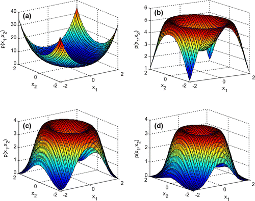
Figure 2. The joint density function of x₁ and x₂: ${\omega }_1=1,{\omega }_2=1.2,{\alpha }_0={\alpha }_1=0.08,{\alpha }_2=0.12,{\beta }_0=0.08,{\beta }_1=0.1,D_2=0.1,D_4=0.12,(a){\beta }_2=0.6,(b){\beta }_2=0.7,(c){\beta }_2=0.8,(d){\beta }_2=0.9.$

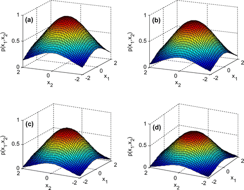
Figure 3. The joint density function of y₁ and y₂: ${\omega }_1=1,{\omega }_2=1.2,{\alpha }_0=0.08,{\alpha }_2=0.12,{\beta }_0=0.08,{\beta }_1={\beta }_2=0.1,D_2=0.1,D_4=0.12,(a){\alpha }_1=0.5,(b){\alpha }_1=0.6,(c){\alpha }_1=0.7,(d){\alpha }_1=0.8.$

Figure 4. The joint density function of y₁ and y₂: ${\omega }_1=1,{\omega }_2=1.2,{\alpha }_0={\alpha }_1=0.08,{\alpha }_2=0.12,{\beta }_0=0.08,{\beta }_1=0.1,D_2=0.1,D_4=0.12,(a){\beta }_2=0.6,(b){\beta }_2=0.7,(c){\beta }_2=0.8,(d){\beta }_2=0.9.$

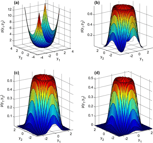
Figure 5. The joint density function of x₁ and x₂: ${\omega }_1=1,{\omega }_2=1.2,{\alpha }_0={\alpha }_1=0.08,{\alpha }_2=0.12,{\beta }_0=0.08,{\beta }_1=0.1,{\beta }_2=0.6,(a)D_2=0.1,D_4=0.12,(b)D_2=0.12,D_4=0.144.$

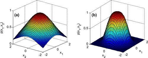
Figure 6. The joint density function of y₁ and y₂: ${\omega }_1=1,{\omega }_2=1.2,{\alpha }_0={\alpha }_1=0.08,{\alpha }_2=0.12,{\beta }_0=0.08,{\beta }_1=0.1,{\beta }_2=0.8,(a)D_2=0.08,D_4=0.96,(b)D_2=0.1,D_4=0.12.$

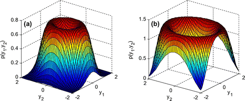
The varieties of joint density function of y₁ and y₂ with the increase of parameters α₁ and β₂ are presented in Figures 3 and 4, respectively. Since the system (1) is coupled, the curved surfaces of joint probability densities are similar to Figures 1 and 2. In detail, Figure 3 is alike Figures 2 and 4 is close to Figure 1, which is because the status of α₁ and β₂ is identical in the coupled oscillator system.

The effects of noise intensities on the joint probability density function are described in Figures 5 and 6. Figures 5 and 6 show that the altitude of peaks and crater raises as the intensities of noises change from D₂ = 0.1, D₄ = 0.12 to D₂ = 0.12, D₄ = 0.144.

4. Almost sure asymptotic stability

When there is only parametric excitation in the system (1), thus, D₂ = D₄ = 0. In this section, we discuss the almost sure asymptotic stability of system (2). According to the theory of stochastic dynamics, the invariant manifold of non-linear dynamical system is tangent with the invariant subspace of its corresponding linear system in equilibrium point, and so almost sure asymptotic stability of the two systems is consistent, which is central conclusion of Oseledec multiplicative ergodic theorem in the theory of stochastic dynamics. Therefore, in order to investigate the stability of coupled Van der Pol oscillator system in the vicinity of equilibrium point, we only need to study the stability of its corresponding linear system. Consider Itô stochastic linearized differential equation of Equation (7)(14) $$\begin{array}{c}\text{d}{z}_1=-({\alpha }_0+D_1/{\omega }_1^2)z_1\text{d}t+(\sqrt{D_1}/{\omega }_1)z_1\text{d}{B}_1(t)\hfill \\ \text{d}{z}_2=-({\beta }_0+D_3/{\omega }_2^2)z_2\text{d}t+(\sqrt{D_3}/{\omega }_2)z_2\text{d}{B}_2(t)\hfill \end{array}$$(14)

Introduce the transformation(15) $$\rho =\left[ln(z_1+z_2)\right]/2,{\varphi }_i=z_i\text{/(}{z}_1+z_2\text{)},i=1,2$$(15)

Obviously, ${\varphi }_i\in [0,1],i=0,1$. The stochastic differential equations for ρ and ϕ₁ can be obtained by Itô lemma and the expression ϕ₂ = 1 − ϕ₁

(16) $$\begin{array}{c}\text{d}\rho =q\left({\varphi }_1\right)\text{d}t+\mathrm{\Sigma }\left({\varphi }_1\right)\text{d}{B}_1(t)\hfill \\ \text{d}{\varphi }_1=m\left({\varphi }_1\right)\text{d}t+\sigma \left({\varphi }_1\right)\text{d}{B}_2(t)\hfill \end{array}$$(16)

where

$q({\varphi }_1)=(c_1-{\beta }_0-D_1{\varphi }_1/2{\omega }_1^2){\varphi }_1/2+[c_2-{\alpha }_0-D_3(1-{\varphi }_1)/2{\omega }_2^2](1-{\varphi }_1)/2,$

$\mathrm{\Sigma }({\varphi }_1)=\sqrt{D_1}{\varphi }_1/2{\omega }_1+(\sqrt{D_3}/2{\omega }_2)(1-{\varphi }_1),$

$m({\varphi }_1)=(c_1-D_3/{\omega }_2^2){\varphi }_1(1-{\varphi }_1)-D_1{\varphi }_1^2(1-{\varphi }_1)/{\omega }_1^2+D_3{\varphi }_1{(1-{\varphi }_1)}^2/{\omega }_2^2,\sigma ({\varphi }_1)=c-{\varphi }_1(1-{\varphi }_1),$

and(17) $$c_1={\beta }_0-{\alpha }_0+D_1/{\omega }_1^2,c_2={\alpha }_0-{\beta }_0+D_3/{\omega }_2^2,c_{\pm }=\sqrt{D_1}/{\omega }_1-\sqrt{D_3}/{\omega }_2.$$(17)

It can be seen from Equation (16(16) $$\begin{array}{c}\text{d}\rho =q\left({\varphi }_1\right)\text{d}t+\mathrm{\Sigma }\left({\varphi }_1\right)\text{d}{B}_1(t)\hfill \\ \text{d}{\varphi }_1=m\left({\varphi }_1\right)\text{d}t+\sigma \left({\varphi }_1\right)\text{d}{B}_2(t)\hfill \end{array}$$(16) ) the process ϕ₁ is independent of variable ρ, and so ϕ₁ is a diffusion process. Thus, the corresponding FPK equation of (15) is as follows:(18) $$\frac{\partial p}{\partial t}=-\frac{\partial }{\partial {\varphi }_1}[m({\varphi }_1)p]+\frac{1}{2}\frac{{\partial }^2}{\partial {\varphi }_1}[\sigma ({\varphi }_1)p].$$(18)

There are two first kind singular boundaries ϕ₁ = 0, 1, and no other singular point exists at 0 < ϕ₁ < 1. Via a simple calculation, we can easily obtain the diffusion index of Equation (16) is 2 and the drift index is 1. ϕ₁ = 0, 1 are both repulsively natural boundaries under the conditions $2c_1>c_{-}^2,2c_2>c_{-}^2$, thus, ϕ₁(t) is ergodic in the interval (0,1) and the stationary probability density of Equation (17) exists. Through the direct integral, one obtains(19) $$p({\varphi }_1)=C{\varphi }_1^{2(c_1/c_{-}^2-1)}{(1-{\varphi }_1)}^{2(c_2/c_{-}^2-1)},{\varphi }_1\in (0,1)$$(19)

where $C=\frac{\Gamma (4\sqrt{D_1{D}_3}/{\omega }_1{\omega }_2{c}_{-}^2)}{\Gamma [(2c_1-c_{-}^2)/c_{-}^2]\Gamma [(c_{+}^2-2c_1)/c_{-}^2]}$.

According to Khasminskii’ theory (Deng & Zhu, 2015), the maximal Lyapunov exponent of system (14) is:(20) $$\begin{array}{c}\lambda ={\int }_0^{1}q({\varphi }_1)p({\varphi }_1)\text{d}{\varphi }_1=[(c_1-{\beta }_0)(2c_1-c_{-}^2)+(c_2-{\alpha }_0)(c_{+}^2-2c_1)]\frac{\mathrm{\Gamma }(4\sqrt{D_1{D}_3}/{\omega }_1{\omega }_2{c}_{-}^2)}{2c_{-}^2\mathrm{\Gamma }(c_{+}^2/c_{-}^2)}\hfill \\ -[c_1{D}_1(2c_1-c_{-}^2)/{\omega }_1^2+c_2{D}_3(c_{+}^2-2c_1)/{\omega }_2^2]\frac{\mathrm{\Gamma }(4\sqrt{D_1{D}_3}/{\omega }_1{\omega }_2{c}_{-}^2)}{2c_{-}^4\mathrm{\Gamma }(2(c_1+c_2)/c_{-}^2)}\hfill \end{array}$$(20)

where $c_1,c_2,c_{\pm }$are shown in Equation (17).

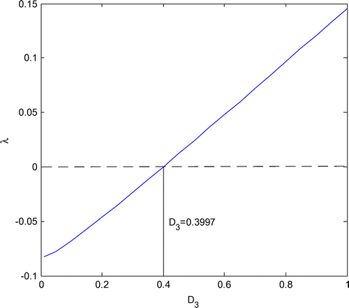
The plan of maximal Lyapunov exponent and noise intensities D₁ and D₃ is given in Figures 7 and 8. The maximal Lyapunov exponents rise with the increased D₁ and D₃, and are less than zero when D₁ < 0.5585 and D₃ < 0.3997, at this moments, the system (1) is almost sure asymptotic stable. Moreover, the maximal Lyapunov exponent increases more quickly in Figure 8 than in Figure 7 as noise intensities are increased.

Figure 7. The plan of the maximal Lyapunov exponent and noise intensityD₁: ${\omega }_1=1,{\omega }_2=1.2,{\alpha }_{0}0.2,{\beta }_0=0.2,D_3=0.1$.

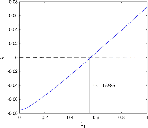
Figure 8. The plan of the maximal Lyapunov exponent and noise intensity D₃: ${\omega }_1=1,{\omega }_2=1.2,{\alpha }_{0}0.2,{\beta }_0=0.2,D_1=0.1$.

5. Conclusion

In this paper, through applying the stochastic averaging method, the averaged FPK equation of coupled Van der Pol oscillator system under the noise excitation is obtained. Moreover, its exact marginal densities are deduced under the compatibility conditions. Then, the effects of the parameters in the system (1) on the marginal densities are discussed. From the Figures 1^{Figure 2Figure 3Figure 4Figure 5}–6, it can be seen that the curved surfaces of density functions decline with the increase of parameters α₁ and β₂, however, the influences of the noise intensities D₁ and D₃ are contrary to them. Finally, the almost sure asymptotic stability of the system (1) is researched through the maximal Lyapunov exponent, and whose analytical expression is derived. Furthermore, the stable boundary point about noise strengths D₁ and D₃ are presented in Figures 7 and 8.

Funding

This work was jointly supported by the Alexander von Humboldt Foundation of Germany (Fellowship CHN/1163390), the National Natural Science Foundation of China (61374080, 11602098), the Natural Science Foundation of Jiangsu Province (BK20161552), Qing Lan Project of Jiangsu, the postdoctoral foundation of Jiangsu Province (1501069B), and the Priority Academic Program Development of Jiangsu Higher Education Institutions.

Additional information

Notes on contributors

Quanxin Zhu

Quanxin Zhu is a professor of Nanjing Normal University, and he has obtained the Alexander von Humboldt Foundation of Germany. Zhu is an associate editor of MPE, JAM, TJMAA, JAAM, RAM and he is a reviewer of Mathematical Reviews and Zentralblatt-Math. Also, Zhu is a senior member of the IEEE and he is the lead guest editor of “Recent Developments on the Stability and Control of Stochastic Systems” in MPE. Zhu has obtained 2011 Annual Chinese and the award of one Hundred “The Most Inuential International Academic Paper”. Moreover, he has been one of most cited Chinese researchers in 2014-2016, Elsevier. Zhu is a reviewer of more than 50 other journals and he is the author or coauthor of more than 110 journal papers. His research interests include random processes, stochastic control, stochastic differential equations, stochastic partial differential equations, stochastic stability, non-linear systems, Markovian jump systems, stochastic complex networks and finance mathematics.

References

- Ariaratnam, S. T., & Xie, W. C. (1994). Almost-sure stochastic stability of coupled non-linear oscillators. International Journal of Non-Linear Mechanics, 29, 197–204.10.1016/0020-7462(94)90038-8
- Ariaratnam, S. T., & Xie, W. C. (1992). Lyapunov exponents and stochastic stability of coupled linear systems under real noise excitation. ASME Journal of Applied Mechanics, 59, 664–673.10.1115/1.2893775
- Arnold, L. (1998). Random dynamical systems. Berlin: Springer.10.1007/978-3-662-12878-7
- Arnold, L., & Papanicolaou, G. (1986). Asympototic analysis of the Lyapunov exponents and rotation numbers of the random oscillator and applications, SIAM. Journal of Applied Mathematics, 46, 427–450.
- Caughey, T. K., & Ma, F. (1982a). The exact steady-state solution of a class of non-linear stochastic systems. International Journal of Non-Linear Mechanics, 17, 137–142.10.1016/0020-7462(82)90013-0
- Caughey, T. K., & Ma, F. (1982b). The steady-state response of a class of dynamical systems to stochastic excitation. Journal of Applied Mechanics, 49, 629–632.10.1115/1.3162538
- Caughey, T. K., & Payne, H. J. (1967). On the response of a class of self-excited oscillators to stochastic excitation. International Journal of Non-Linear Mechanics, 2, 125–151.10.1016/0020-7462(67)90010-8
- Deng, M. L., & Zhu, W. Q. (2015). Stochastic averaging of quasi-non-integrable Hamiltonian systems under fractional Gaussian noise excitation. Nonlinear Dynamics, 83, 1015–1027.
- Doyle, M. M., & Namachchivaya, N. S (1994). Almost-sure asymptotic stability of a general four-dimensional system driven by real noise. Journal of Statistical Physics, 75, 525–552.10.1007/BF02186871
- Itô, K. (1951). On stochastic differential equations memoris. American Mathmatical society, 4, 1–51.
- Khasminskii, R. Z. (1967). Necessary and sufficient conditions for the asymptotic stability of linear stochastic systems. Theory of probability and application, 11, 144–147.10.1137/1112019
- Khasminskii, R. Z. (1968). On the averaging principle for Itô stochastic differential equations. Kibernetka, 3, 260–279.
- Li, S. H., & Liu, X. B. (2012). The maximal Lyapunov exponent of a co-dimension two-bifurcation system excited by a bounded noise. Acta Mechanica Sinica, 28, 511–519.10.1007/s10409-012-0013-y
- Lin, Y. K., & Cai, G. Q. (1995). Probabilistic structural dynamics. Advanced theory and applications. New York, NY: McGraw-Hill.
- Liu, X. B., & Liew, K. M. (2004). The maximal Lyapunov exponent for a three-dimension stochastic system, ASME. Journal of Applied Mechanics, 71, 677–690.
- Liu, W. Y., & Zhu, W. Q. (2013). Stochastic stability of quasi non-integrable Hamiltonian systems under parametric excitations of Gaussian and Poisson white noises. Probabilistic Engineering Mechanics, 32, 39–47.
- Liu, W. Y., & Zhu, W. Q. (2014). Stochastic stability of quasi-integrable and resonant Hamiltonian systems under parametric excitations of combined Gaussian and Poisson white noises. International Journal of Non-Linear Mechanics, 77, 52–62.10.1016/j.ijnonlinmec.2014.08.003
- Liu, W. Y., & Zhu, W. Q. (2015). Lyapunov function method for analyzing stability of quasi-Hamiltonian systems under combined Gaussian and Poisson white noise excitations. Nonlinear Dynamics, 81, 1–15.
- Mitchell, P. R., & Kozin, F. (1974). Sample stability of second order linear differential equations with wide band noise coefficients, SIAM. Journal of Applied Mathematics, 27, 571–605.
- Namachchivaya, N. S., Vedula, L., & Onu, K. (2011). Stochastic stability of coupled oscillators with one asymptotically stable and one critical mode. Journal of Applied Mechanics, 78, 2388–2399.
- Nishoka, K. (1976). On the stability of two-dimensional linear stochastic systems. Kodai Mathematical Seminar Reports, 27, 211–230.
- Zhao, Y. P. (2015). An improved energy envelope stochastic averaging method and its application to a nonlinear oscillator. Journal of Vibration and Control, 21, 1–12.
- Zhu, W. Q., Cai, G. Q., & Lin, Y. K. (1990). On exact stationary solutions of stochastically perturbed Hamiltonian systems. Probabilistic Engineering Mechanics, 5, 84–89.10.1016/0266-8920(90)90011-8
- Zhu, W. Q., Cai, G. Q., & Lin, Y. K. (1992). Stochastically perturbed haniltonian systems nonlinear stochastic mechanics, proceedings of IUTAM symposium (pp. 543–552). Berlin: Springer-Verlag.
- Zhu, W. Q., Huang, Z. L., & Suzuki, Y. (2001a). Response and stability of strongly nonlinear oscillators under wide band random excitation. International Journal of Non-Linear Mechanics, 36, 1235–1250.10.1016/S0020-7462(00)00093-7
- Zhu, W. Q., Huang, Z. L., & Suzuki, Y. (2001b). Exact stationary solutions of stochastically excited and dissipated partially integrable Hamiltonian systems. International Journal of Non-Linear Mechanics, 36, 39–48.10.1016/S0020-7462(99)00086-4
- Zhu, W. Q., Huang, Z. L., & Suzuki, Y. (2002). Stochastic averaging and Lyapunov exponent of quasi partially integrable Hamiltonian systems. International Journal of Non-Linear Mechanics, 37, 419–437.10.1016/S0020-7462(01)00018-X
- Zhu, W. Q., Huang, Z. L., & Yang, Y. Q. (1997). Stochastic averaging of quasi-integrable Hamiltonian systems. Journal of Applied Mechanics, 64, 975–986.10.1115/1.2789009