Determinants of peri-urban households' livelihood strategy choices: An empirical study of Bahir Dar city, Ethiopia

Abstract

Agriculture is the dominant economic activity and the primary source of livelihoods for Bahir Dar city peri-urban farm households. However, due to urbanization, farmers have been forced to be displaced from their farm landholding system. This article examines determinants of households’ livelihood strategy choices and impact analysis of urbanization of Bahir Dar city on peri-urban households’ livelihood strategies. A stratified sampling technique was employed to select 310 households for primary data collection. The data were subjected to both descriptive and econometric techniques of analysis. Multinomial logit regression analysis was used to identify determinates of households' livelihood strategy choice and propensity score matching (PSM) to examine the impact of urbanization on households' livelihood strategy. From PSM analysis, the effect of displacement on households’ livelihood outcome has a negative difference of −0.118316729 as compared to non-displacement. From the total respondents, 216 (69.67%) households depend solely on farm work self-employment strategy, 54 (17.42%) respondents participate in non-farm self-employment strategy, 10 (3.23%) respondents participate in informal wage work strategy, and 30 (9.68%) respondents participate in formal wage strategies. Multinomial logit regression shows that households’ livelihood choice was positively and significantly influenced by household age, household education level, and dependency ratio at 10% level of significance and household size at 1% level of significance. But household head sex (P < 0.01), household land size, and household access to credit (P < 0.001) influence negatively their livelihood choice. The findings of this study suggest that policymakers need to reflect on the most suitable way of mitigating negative impacts of farmland loss on peri-urban areas.

Keywords:

• impact
• PSM
• determinants
• binary logit regression
• peri-urban area
• Ethiopia

PUBLIC INTEREST STATEMENT

The world population has continued predominantly urban, and the world has gone through a process of rapid urbanization over the past six decades. In 1950, more than 70% of the people worldwide were subsisted in rural settlements and less than one-third in urban settlements. In 2014, 54% of the world’s population was urban. The urban population is expected to continue to grow. Levels of urbanization vary significantly across regions. In 2014, high levels of urbanization, at or above 80%, characterized Latin America and Northern America and Africa in contrast, remain mostly rural, with 40% and 48% of their respective populations living in urban areas. Urbanization in Africa and Ethiopia from 1950 to 2005 grew from 14.5 to 37.9 and 4.6  to 16.1, respectively. Urbanization in Ethiopia is very low compared to Africa, but the annual rate of change within this period is 1.72 and 2.32%, respectively.

1. Introduction

The process of urbanization is a worldwide phenomenon recorded in the history of all urban centers and has been estimated before the beginning of the nineteenth century. It started with the earliest human civilization of Babylonians (Fransen, Kassahun, & van Dijk, 2010). At the macro level, urbanization is defined as the increase in the concentration of population in urban areas both relatively and absolutely (Fazal, 2000; Kasa, Zeleke, Alemu, Hagos, & Heinimann, 2011). At the same time, urbanization is also referred to as the increasing share of a nation’s population living in urban areas. Often, urbanization is the result of net rural to urban migration. The level of urbanization is the share itself, and the rate of urbanization is the rate at which that share is changing (Satterthwaite, McGranahan, & Tacoli, 2010). The demographic and economic expansions of cities, through processes such as migration and industrialization, tend to be accompanied by spatial expansion, resulting in encroachments by cities upon adjacent peri-urban areas (Gullette, Thebpanya, & Singto, 2017; Oduro, Adamtey, & Ocloo, 2015). This process is the outcome of social, economic, and political developments that lead to urban concentration and growth of large cities, changes in land use, and transformation from rural to metropolitan pattern of organization and government. Hence, urbanization affects all spheres of human life of both rural and urban setting (Naab, Dinye, & Kasanga, 2013; Pauchard, Aguayo, Peña, & Urrutia, 2006).

Ethiopia is the second most populous country of the African continent next to Nigeria and is one of the least urbanized countries in the world (Adam, 2014, 2016). Ethiopia stands out as a country that is both rapidly urbanizing and particularly impoverished. The share of the population living in cities has increased from an estimated 7.1% in 1994 (Schmidt & Kedir, 2009) to 16% in 2008 (Abebe, 2006) and is expected to reach 60% by 2040 at the current annual growth rate of 3.5% (Desa, 2014). So, the next three decades are the ones in which Ethiopia will be building its cities with which it may then have to live for many generations. Ethiopia faces this daunting task as one of the poorest countries on earth, with a per capita GDP of less than US$600—far below the 2014 average in sub-Saharan Africa (excluding South Africa) of US$1699 (Schmidt & Kedir, 2009). However, given the 2.73% total annual population growth rate, high rate of in-migration to towns, and increase in the number of urban centers, the rate of urbanization is increasing at a rate of 4.4% (Tadesse & Headey, 2010). Furthermore, the country’s urban population is expected to grow on average by 3.98%, and by 2050, about 42.1% of the total population is expected to be inhabited in urban centers (Tessema, 2017; Un-habitat, 2010).

Urbanization in Bahir Dar city is in a state of rapid horizontal expansion. It increased from 1957 to 2009 at an average growth rate of about 31% (88 ha/year) (Haregeweyn, Fikadu, Tsunekawa, Tsubo, & Meshesha, 2012). This will have far-reaching ecological, socio-economic, and environmental consequences, especially to the urban fringe areas. Particularly, the main challenge of the urbanization process in the study area is the rapid conversion of a large amount of prime agricultural land to urban land uses (mostly residential construction) in the peri-urban areas. It can affect the unavailability of prime agricultural land and consequently exposes for low agricultural productivity and low standard of living (Francis, 2013; Shishay, 2011). This trend will exacerbate further expropriation of farm households and may lead to food insecurity and social instability in the surrounding areas. Policies that ensure a just and equitable compensation for such expropriated farmers still remain necessary (Z. Muluwork, 2014). Hence, a better understanding of the spatial and temporal dynamics of urban growth and its impact on the small-scale farmer’s life in the study area will be required. Currently, Bahir Dar expands dramatically, and the demand of land for urban development program increases rapidly with non-existent urbanization process. In response to these, the government is taking large tracts from peri-urban areas. As a result, large numbers of local landholders who mainly engage in agricultural activity for their livelihood have been forced to lose their land rights (Achamyeleh, 2014). Therefore, this condition indicates the researchers to perform the research on determinants of households’ livelihood strategy choices and impact analysis of urbanization of Bahir Dar city on peri-urban households’ livelihood strategies.

2. Review of related literature

2.1. Pattern and trend of urban growth in Ethiopia

Ethiopia is currently of the least urbanized countries in the world even Africa. Less than one person in five is a city or town dweller. However, the rate of at which the countries urban areas the growing are among the highest in Africa. Many social, economic, and environmental problems have accomplice urbanization in Ethiopia and have been ignored for too long (Kebbede, 2017). The people residing in urban areas also increasing from 4–3 million in 1987 to 7–4 million in 1994, which is estimated to have already reached 10–6 million in the year 2003 and projected to reach 20 million by the year 2020 (Kasa et al., 2011) (see Figure 1).

2.2. Impacts of urbanization

As activities develop, effects can include a dramatic increase and change in costs often pricing the local working class out of the market including such functionality as employs of the local municipalities (Tessema, 2017). Urban problems along with infrastructure developments are also fueling suburbanization trends in developing nations through the trends for core cities inside nations tend to continue to become ever denser (Glaeser & Steinberg, 2017) (Figure 2).

Peri-urban areas surrounding the urban areas are characterized as one of the most vulnerable geographic areas for the risk subjected to farmland loss in the expansion of urbanization that makes farmers loss of livelihood assets (B. B. Muluwork, 2014). The expansion of urban areas over natural resources and agro productive system has been a characteristic process which has resulted in the emergence of new landscapes with mixed urban and rural features (Satterthwaite et al., 2010).

3. Research methodology

3.1. Description of the study area

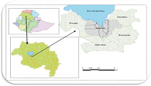
Bahir Dar city has a long history dated back to at least the sixteenth or seventeenth century and at this moment the capital of Amhara National Regional State (ANRS) which is located on the southern shore of Lake Tana, the source of Blue Nile (Abay) river in the northwestern part of Ethiopia (see Figure 3). A global position of the city is between 15.620 N latitude and 37.420 E longitude and enjoys the tropical type of climate with an average annual temperature of 19.60°C, and the average elevation of the city is estimated 1,801 m above sea level. Topographically, the city lies on a flat surface with almost no slope gradient except for small increases in elevation in the eastern and western peripheries. The city is distinctly known for its wide avenues lined with palm trees and a variety of colorful flowers (Daniel, 2011; Haregeweyn et al., 2012). Bahir Dar city is one of the fastest-growing urban centers in Ethiopia both demographically and spatially. The amount of land demanded for different urban development purposes is increasing every year. Based on CSA, in 1994 (96,140) and 2007 (220, 344) (CSA, 2007) and according to ANRS bureau of finance and economic development in 2014 estimated (297,749) the data reveals that within 20 years the population of the city has increased by more than 200,000 people and interims of physical size an overlay of Bahir Dar administrative boundaries increase with an annual increment of 31%, from 279 ha in 1957 to 4,830 ha in 2009 (Haregeweyn et al., 2012), built-up areas increased as a result of horizontal expansion.

Figure 1. Ethiopia urbanization trend and projection to 2050. Source (Eastwood & Lipton, 2011)

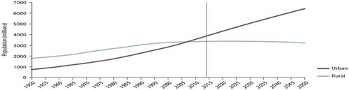
Figure 2. Conceptual framework for the analysis of Bahir Dar city peri-urban household livelihoods. Source: Adopted from DFID's sustainable livelihood framework (DfID, UK, 1999) and sustainable rural livelihood framework (Tuyen, Lim, Cameron, & Huong, 2014)

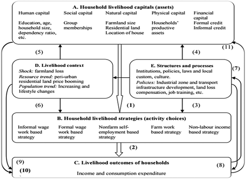
Figure 3. Map of Bahir Dar City Administration and peri-urban areas

3.2. Data types and source

In order to attain the objectives of this research, all required data were collected from both primary and secondary data sources. The study was conducted primary data sources from sample households using a pre-tested structured questionnaire by applying face-to-face interview to reduce nonresponse rate and incompleteness of data. Secondary data were collected from published and unpublished materials including websites.

3.3. Sample size and sampling techniques

Bahir Dar city is surrounded by four peri-urban Kebeles, such as “Weramit”, “Zenzelima”, “Addis Alem”, and “Woreb Kola”. The choice of sampling technique (probability or non-probability) depends on the purpose of the study. So, the objective of this study is to estimate households’ solid waste generation and management behavior in the case of Bahir Dar city. For such a quantitative research, a probability sampling technique is appropriate as compared to non-probability sampling technique because it gives equal chance of being interviewed for every sample household. From different techniques of probability sampling for this study, two-stage sampling was used.

3.3.1. First stage: Selection of Sample gotes

From the existing four Kebeles, a total of four gotes (smallest administrative units in rural Kebeles) were selected randomly by applying Lottery method as a sample, i.e., one gote from each kebele, since each kebele has more or less equal gotes. To select the sample gotes, first the existing sub-kebele gotes make sample frame.

3.3.2. Second stage: Selection of households

Sample households are the main primary data sources of this study. But determining the research sample size is a function of different factors like resource, time, the purpose of the study, characteristics of the population, etc. So, to determine the sample size, we used scientific formula, and a critical component of sample size formulas is the estimation of variance in the primary variables of interest in the study (Cochran, 1977). For categorical dependent variable, 5% margin of error is acceptable, and for continuous dependent variable, 3% margin of error is acceptable (Krejcie & Morgan, 1970). The formula that we used for determining sample size is the following formula adopted from Israel (1992).

(1) $n=\frac{N}{1+N\left(e^2\right)}$(1)

where n = minimum required sample size, N = population size, and e = level of precision.

Therefore, based on the above-specified formula, the required sample size becomes:

$n=\frac{1365}{1+1365\left({0.05}^2\right)}\approx 310$

Stand on this, a total sample of 310 households from which 149 displaced and the remaining 161 non-displaced (control group) were selected randomly from generated strata sampling frame from roasters of each kebele administration office proportional to the displaced sample size (see Table 1).

3.4. Method of the data analysis

Quantitative and qualitative data gathered through different tools were processed both manually and electronically (propensity score matching (PSM) and binary logit model) and were used to analyze the determinants of peri-urban households' livelihood choice and urbanization impact on households' livelihood. Quantitative data that were collected from sample households should be processed and analyzed using data analysis statistical software STATA version 13. These were done after appropriate coding, edited, and register of collected data and then enter the data into STATA software. The findings from the analysis were presented by using descriptive statistics (quantitative methods) which includes mean, frequency distribution tables, percentages, and standard deviation methods. Finally, conclusion and recommendation were formulated based on findings.

3.4.1. Impact assessment

In determining the impact of an intervention, an impact assessment must estimate the counterfactual; that is, what would have happened had the intervention or program never taken place or what otherwise would have been. To determine the counterfactual, it is essential to net out the effect of the intervention from other factors. This is accomplished through the use of control groups which are compared with the treatment group. The choice of a good counterfactual is therefore crucial in impact assessment. PSM is an alternative method to estimate the effect of receiving treatment when the random assignment of treatments to subjects is not feasible. The PSM method compares the outcome of a treated observation with the outcomes of comparable non-treated observations. To match the treated with the non-treated, we have to choose a matching algorithm. Hence, the success of PSM hinges critically on the data available, as well as the variables used for matching (Diaz & Handa, 2004). As a program evaluation technique, PSM is based on the idea of comparing the outcomes of program participants with the outcomes of “equivalent” non-participants. The estimated propensity score (PS), for subject e (Xi), (i = 1 … N) is the conditional probability of being assigned to a particular treatment given a vector of observed covariates Xi (Rosenbaum & Rubin, 1983):

2 $e\left(xi\right)=pr\left(zi=1|xi\right)$2

3 $pr(Zi,---,x_1,---x_n)=\sum _{i-1}^{n}e(xi{)}^{zi}(1-e(xi{)}^{1-zi})$3

where

• Zi = 1 for treatment; Zi = 0 for control; Xi = the vector of observed covariates for the $i^{th}$ subject.

The PS is a probability, and it ranges in values from 0 to 1. Thus, if PSM was used in a randomized experiment comparing two groups, then the PS for each participant in the study would be 0.50. This is because each participant would be randomly assigned to either the treatment or the control group with a 50% probability. This study designs there is no randomization, such as in a quasi-experimental design, and the PS must be estimated. PS values are dependent on a vector of observed covariates that are associated with the receipt of treatment.

In this study, PSM was used to evaluate the impact of urbanization on livelihood outcomes of the peripheral farming community. If $Y_1$ denotes the potential outcome conditional on participation and $Y_0$ denotes the potential outcome conditional on nonparticipation; the impact of the program is given by:

4 $\mathrm{\Delta }=Y_1-Y_0$4

i. Estimating the propensity score (PS)

The PS is defined as the conditional probability of receiving a treatment given pretreatment characteristics (Rosenbaum & Rubin, 1983). The PSs were computed using binary logit regression models given as:

5 $P\left(X\right)=Pr\left\{D=1/X\right\}=E\left\{D/X\right\}$5

where

• D = (0, 1) is the indicator of exposure to treatment characteristics (dependent variable). That is, D = 1, if exposed to treatment (displaced) and D = 0 if not exposed to treatment;

• X is the multidimensional vector of observed characteristics (explanatory variables).

ii. Matching the unit using the propensity score

After the PS is estimated and the score computed for each unit, the next step is the actual matching. In this study, we use the nearest neighbor score of similar individuals in the treated and control groups to construct the counterfactual outcome. So, the nearest neighbor matching method was used to match in this study. One major advantage of this approach is the lower variance which is achieved because more information is used as compared to others (Appendix). The matching estimator is given as:

6 ${\tau }^M=\frac{1}{N^T}\sum iET\left\{Y_i^T-\sum iET{W}_{ij}{Y}_j^c\right\}=\frac{1}{N^T}\left\{\sum iET{Y}^T-\sum iET\sum iET{W}_{ij}{Y}_j^c\right\}$6

$i,E,T,N_i^c$ denote the numbers of controls matched with observation and define the weights $W_{ij}=\frac{1}{N_i^c}$ and $W_{ij}=0$ otherwise.

M stands for the nearest neighbor matching, and the number of units in the treated group is denoted by$N^T$. One of the major advantages of this method is that the absolute difference between the estimated PSs for the control and treatment groups is minimized.

iii. Estimating the impact (average treatment effect on the treated)

The matched sample was used to compute the average treatment effect for the treated (impact).

It is estimated as follows:

7 $ATT=E\left(\mathrm{\Delta }|D=1,X\right)=E\left(Y_1-Y_0|D=1,X\right)=E\left(Y_1|D=1,X\right)-E\left(Y_0|D=0,X\right)$7

where D = 1 denotes the program participation (displaced) and Χ is a set of conditioning variables on which the subjects were matched. Equation 77 $ATT=E\left(\mathrm{\Delta }|D=1,X\right)=E\left(Y_1-Y_0|D=1,X\right)=E\left(Y_1|D=1,X\right)-E\left(Y_0|D=0,X\right)$7 would have been easy to estimate except for the equation Ε (Y0 | D = 1, X). This is the mean of the counterfactual and denotes what the outcome would have been among participants had they not participated in the program (non-displaced).

Given that the conditional independence assumption and the common support assumption holds, then we estimate the mean effect of the treatment through the mean difference in the outcomes of the matched pairs:

8 $ATT=\frac{1}{N_1}\sum _{i=1}^{N_1}\left(y_{1i}-\sum _{j=1}^{N_0}{w}_{ij}{y}_{0j}\right)$8

A weighted average of all displaced outcome variables is subtracted from every non-displaced outcome variable.

where $\sum _{j=1}^{N_0}{w}_{ij}=1$

• $N_1=$number of displaced; $N_0$ = number of non-displaced; $i=$index of displaced; $j=$index of non-displaced; and $W_{ij}=$weights.

3.4.2. Multinomial logit model specification

When there is a dependent variable with more than two alternatives among which the decision-maker has to choose (i.e., unordered qualitative variables). For this study, therefore, a multinomial logit model makes it possible to analyze factors influencing of households’ livelihood strategy choices in the context of multiple choices. Following Greene (2003), suppose for the$i^{th}$ respondent faced with j choices, we specify the utility choice j as:

9 $U_{ij}=Z_{ij}\beta +{\epsilon }_{ij}$9

If the respondent makes choice j in particular, then we assume that $U_{ij}$is the maximum among the j utilities. So the statistical model is derived by the probability that choice j is made, which is$Pr(U_{ij}>U_{ik})$ for all other k$\ne$j

where $U_{ij}$ is the utility to the $i^{th}$ respondent form livelihood strategy j $U_{ik}$ the utility to the $i^{th}$ respondent from livelihood strategy k if the household make the most its utility defined over income comprehensions, then the household’s choice is simply an optimal allocation of its asset bequest to choose livelihood that makes the best use of its utility (Brown & Brown et al., 2006). Thus, the $i^{th}$ household’s decision can, therefore, be modeled as maximizing the predictable utility by choosing the $i^{th}$ livelihood strategy among J discrete livelihood strategies, i.e.:

10 $\underset{j}{max}=E(u_{ij})=f_i(x_i)+{\in }_{ij};j=\mathrm{0....}J$10

In general, for an outcome variable with J groups, let the $J^{th}$ livelihood strategy that the $i^{th}$ household chooses to maximize its utility could take the value 1 if the $i^{th}$ household chooses $J^{th}$ livelihood strategy and 0 otherwise. The probability that a household with characteristics x chooses livelihood strategy j, $p_{ij}\hspace{0.17em}$ is modeled as:

11 $P_{ij}=\frac{\mathrm{e}\mathrm{x}\mathrm{p}\left(X_{i\hspace{0.17em}}{\beta }_j\right)}{{\sum }_{j=0}^j\mathrm{e}\mathrm{x}\mathrm{p}\left(X_i{\beta }_j\right)},J=0$11

With the requirement that ${\sum }_{j=0}^j{p}_{ij}=1$ for any i

where

• $P_{ij}$ = probability in place of the $i^{th}$ respondent’s chance of falling into group j

• X = predictors of response probabilities (Table 2)

• ${\beta }_j=$Covariate effects specific to $j^{th}$ response category with the first category as the reference.

Proper standardization that eliminates an indeterminacy in the model is to assume that ${\beta }_1$ = 0 (this rise is because probabilities sum to 1, so only J parameter vectors are desirable to determine the J +1 probabilities) (Galab et al., 2002) so that exp ($x_i{\beta }_1$) = 1. Suggesting that the generalized Equation (11)11 $P_{ij}=\frac{\mathrm{e}\mathrm{x}\mathrm{p}\left(X_{i\hspace{0.17em}}{\beta }_j\right)}{{\sum }_{j=0}^j\mathrm{e}\mathrm{x}\mathrm{p}\left(X_i{\beta }_j\right)},J=0$11 is equal to:

$Pr\left(y_{i\hspace{0.17em}}=\frac{j}{X_i}\right)=P_{ij}=\hspace{0.17em}\frac{exp\left(X_{i\hspace{0.17em}}{\beta }_{j\hspace{0.17em}}\right)}{1+{\sum }_{j=0}^{j}exp\left(X_{i\hspace{0.17em}}{\beta }_{j\hspace{0.17em}}\right)},J=0,1,2\dots j$

(12) $\mathrm{P}\mathrm{r}(y_i=\frac{1}{X_i}=\hspace{0.17em}\frac{1}{1+{\sum }_{j=1}^{j}exp\left(X_i{\beta }_j\right)}$(12)

where y = A polychromous result variable with groups coded from 0, J.

Note: The probability of $P_{i1}$is derived from the constraint that the J probabilities sum to 1. That is, $\sum P_{ij}=1$.

4. Result

PSM, multinomial logit, and binary logit econometric models were employed to analyze whether there is a significant difference between displaced and non-displaced in terms of livelihood outcome and livelihood strategy choice of displaced farming community measured in weighted average livelihood outcome strategy.

The result given in Table 3 shows that there is a statistically significant difference between displaced and non-displaced in terms of household land size, education of working member, household size, and the total value of the current productive asset and were significant at 1%, while male working member and dependency ratio are significant at 10% probability level. In addition, the result also revealed that there is no statisticallysignificant difference between displaced and non-displaced in terms of land per adult and group membership. Non-displaced households on average have 57.1% and 16.05% higher in landholding size and dependency ratio than those of the displaced household, respectively, and in contrast to the non-displaced sampled households, displaced households have large numbers of household size, large number of male working members, better level of work education, and larger value of current total productive asset.

Table 1. Population and sample size of each peri-urban kebele

Peri-urban Kebele	Sample gote	Total number of households estimated	Estimated displaced households	Household % share for displaced	Sample for displaced	Sample for non-displaced
Weramit	Lumame	338	115	19	29	37
Zenzelima	Sesaberet	535	266	44	65	68
Addis Alem	Qutatina	351	169	28	42	44
Woreb Kola	Chorqa	141	54	9	13	12
Total	4 gotes	1,365	604	100	149	161

Source: Kebeles Administration offices (2017)

Table 2. Definition and measurement of independent variables in PSM and MNLM logit model

Variable	Definition	Measurement	Hypothesis
Definition and measurement of independent variables used in the PSM model
head-sex	Sex of household head	1 =Male, 0 otherwise	Positive
head_educ	Educational level of the household head	Level category	Positive
wor-educ	Average years of formal schooling of adult members who were employed in the last 12 months	Years	Positive
hhs-si	House hold family size	Number	Positive
mal-wor	Number of male adult members who were employed in the last 12 months	Number	Positive
dep-ratio	The ratio of unemployed to labor force	Ratio	Negative
hhslan_size	Household agricultural landholding size	Hectares	Positive
Lan-ada	Owned farm size per member aged 15 and over	Hector	Positive
totvalcur-ass	Value of all productive assets	Birr	Positive
gro-mem	Number of memberships in formal and informal groups and organizations	Number	Positive
(2) Definition and measurement of independent variables used in MNLM			Hypothesis
head-sex	Sex of household head	1 =Male, 0 otherwise	Positive
head-age	Age of household head	Years	Negative
head-educ	Educational level of the household head	Level category	Positive
hhs-si	Family size of household	Number	Positive
dep-rat	The ratio of unemployed to labor force	Ratio	Positive
gro-mem	Number of memberships in formal and informal groups and organizations	Number	Positive
hhslan- size	Household agricultural landholding size	Hectares	Negative
totvalcur-ass	Value of all productive assets	Ethiopian birr	Negative
Acc_cre	Access to formal and informal credit	Dummy (=1 if yes)	Positive

Table 3. Summary statistics and mean difference test on the continuous variable

	Non-displaced (N =161)		Displaced (N =149)		Total (N =310)		Mean difference
Explanatory variables	Mean	(SD)	Mean	(SD)	Mean	(SD)	Mean	(SD)	T-value
wor_edu	2.579	2.476	3.497	2.619	3.020	2.583	−0.918	−13.11	0.07 ***
hhs_si	5.267	1.749	5.718	1.725	5.484	1.749	−0.451	1.45	−0.31***
mal_wor	1.839	1.012	1.966	1.093	1.900	1.052	−0.128	−0.14	0.92*
dep_rat	64.93	50.06	55.95	42.68	60.61	46.80	8.99	26.44	0.34*
hhslan_size	1.769	0.938	1.126	0.785	1.460	0.925	0.643	−1.04	−0.62***
lan_ada	0.557	0.340	0.311	0.253	0.439	0.325	0.246	−0.34	−0.72
totval_curprass	75,307	45,471	78,860	75,377	77,015	61,604	−3554	−4442	0.08***
gro_mem	2.422	0.739	2.416	0.789	2.419	0.762	0.006	0.01	0.49

***, **, and * are significant at 1%, 5%, and 10% significance levels, respectively.

Source: survey result (2017).

The descriptive analysis of Pearson’s chi-square proportion difference test between displaced and non-displaced for categorical variables (Table 4) shows that there is a significant difference between displaced and non-displaced in terms of household head education level at 10% levels of significance in addition to the total sampled households, and 61%, 21%, 11%, and 7% are illiterate, primary, junior, and secondary and above, respectively. This implies that household education has an effect on livelihood outcome difference. However, there is no significant difference between displaced and non-displaced in sex.

Table 4. Summary statistics and proportional difference test between categorical variables

Variables	Category	Non-displaced (N =161)		Displaced (N =149)		Total (N = 310)		X^2
		N	%	N	%	N	%
head_sex	Male	144	89.44	123	82.55	267	86.13	0.742
	Female	17	10.56	26	17.45	43	13.87
head_educ	Illiterate	89	55.28	100	67.11	189	60.97	2.685*
	Primary	39	24.22	27	18.12	66	21.29
	Junior	22	13.66	11	7.38	33	10.65
	Secondary and above	11	6.83	11	7.38	22	7.10

***, **, and * are significant at 1%, 5%, and 10% significance levels, respectively.

Source: survey result (2017).

4.1. Estimation of propensity scores

The binary logit regression model was employed to estimate PSs for matching displaced household with control or non-displaced households. For estimating PSs only those variables which affect both the likelihood of displacement and the outcomes of interest were included.

The pseudo-R² value 0.2501 shows that the competing households do not have many distinct characteristics overall, so finding a good match between the treated and non-treated households becomes easier. The maximum likelihood estimate of the logit regression model result (Table 5) shows that displacement status has been significantly and negatively affected by household land size, education of household head, male working number, and dependent ratio and was significant at 1% significance level (P <0.001), and it is positively affected by working education, household size, and total value of the current productive asset which are significant at equally 1% significant level. Meaning those peri-urban farming communities who displaced due to urban expansion, have better work educational member in the household being engage in the formal wage work employment, this would have positively influenced for sustainable livelihood outcome. Similarly, households having larger family sizes have excess labor to participate in income-generating activities.

Table 5. Logistic regression model result for displacement status

Explanatory variable	Coefficients	Z-value
_cons	−.4075301	−0.51
head_sex	−.2516155	−0.56
head_educ	−.3107563	−1.93*
wor_edu	.257916	3.33***
hhs_si	.5138804	3.01***
mal_wor	−.3722243	−1.76*
dep_rat	−.0089635	−1.66*
hhslan_size	−2.07851	−4.31***
lan_ada	.7194893	0.58
totval_cur~s	9.11e-06	2.60***
gro_mem	.3051199	1.54
Number of observations 310; LR chi2(10) = 107.35 Prob> chi2 = 0.0000 Log likelihood = −160.9686 Pseudo R^2 = 0.2501

***, **, and * significant at 1%, 5%, and 10% significance levels, respectively

Source: survey result (2017).

4.2. Impacts of displacement on peri-urban households

This section presents evidence whether the displacement has brought significant changes in the livelihood outcome of the peri-urban farming communities. After controlling for other characteristics, the PSM model using the nearest neighbor matching estimator result indicates (Table 6) that there is an insignificant difference in livelihood outcome of displaced farming community by −0.118316729 as compared to the non-displaced farming community.

Table 6. Impacts of urban expansion displacement on the farming community

Outcome variables	Displaced	Controls	Difference	SE^B	T-value
Livelihood outcome	2.93758389	3.05590062	−.118316729	.044381367	−2.67

Source: Own result (2017).

4.3. Household livelihood strategies

Table 7 describes the number of households in the past and current livelihood strategy choice. Concurrently, the number of households predominantly who pursue non-farm self-employment and informal and formal wage work livelihood strategies considerably increased. This means that comparatively there was a more profound transition from the farm work-based strategy to the non-farm-based (B, C, and D) strategies among the displaced households than non-displaced households. This suggests that the loss of farmland may have a considerable effect on the choice of household livelihood strategy.

Table 7. Households' past and current livelihood strategies

Change in current livelihood strategies of households
	Whole sample		Displaced households		Non-displaced households
Livelihood strategies	Past	Current	Past	Current	Past	Current
Farm work self-employment (A)	293	216	142	76	151	140
Non-farm self-employment (B)	11	54	4	42	6	12
Informal wage work (C)	3	10	1	6	2	4
Formal wage work (D)	4	30	2	25	2	5
Total	310	310	149	149	161	161

Source: own survey result, 2017.

From the total 310 sample respondents, 216 (69.67%) households depend solely on farm work self-employment strategy (crop, plant, and animal production), 54 (17.42%) respondents participate in non-farm self-employment strategy (sale of wood or charcoal, stone, weaving, pottery, metal works, sale of local drinks, small business venture/shop, etc.), 10 (3.23%) respondents participate in informal wage work strategy (without a formal labor contract mainly daily laborer), and 30 (9.68%) respondents participate in formal wage strategies (with a formal labor contract mainly guard and office work). Based on this survey result, we can conclude that most of the peri-urban area households predominantly engaged only in farming activities rather than the other livelihood strategies.

Table 8 describes the number of households in the past and current livelihood activity choice.

Table 8. Households' past and current livelihood activities

Change in livelihood activities of households
Livelihood activities	Whole sample		Displaced households		Non-displaced households
	Past	Current	Past	Current	Past	Current
Agricultural only (1)	218	94	112	24	106	70
Agriculture + handcrafts, sale of wood or charcoal, sale of stone shops, etc. (2)	37	120	18	72	19	48
Agriculture + daily laborer (3)	26	28	7	13	19	15
Agriculture + office work and guard (4)	25	44	9	21	16	23
Agriculture + handcrafts, sale of wood or charcoal, sale of stone shops + daily laborer (5)	0	1	0	1	0	0
Agriculture + handcrafts, sale of wood or charcoal,sale of stone shops, etc., + office work and guard (6)	2	14	1	11	1	3
Agriculture + daily laborer + office work and guard, etc. (7)	1	5	1	3	0	2
Agriculture + handcrafts, sale of wood or charcoal, sale of stone shops, etc., + daily laborer + office work and guard (8)	1	4	1	4	0	0
Total	310	310	149	149	161	161

Source: Own survey (2017).

In general, whole sample, the number of households who pursue 2–8 livelihood strategy activities considerably increased. Comparatively, there was a more profound transition from farm works only to the other diversified activity choices (2–8) among the displaced households than that among the non-displaced households. This also suggests that the loss of farmland may have a considerable effect on the choice of household livelihood strategies.

Table 9 presents livelihood income distribution under various types of livelihood strategies. The mean livelihood income of the displaced household was less than a non-displaced household on average by 333.17 ETB.

Table 9. Mean household income and percentage composition by current livelihood strategy

Displacement status		Income by livelihood strategies
		Total	A	B	C	D
Displaced	Mean	33,517.65	19,107.21	20,705.32	12,063.16	10,338.86
	SD	27,753.89	12,665.29	36,651.9	6441.55	5846.56
Non-displaced	Mean	33,850.82	26,647.3	14,108.16	11,094.12	10,764.08
	SD	15,166.94	14,175.76	9122.09	7633.19	5087.89
Total	Mean	33,690.68	23,048.62	18,139.76	11,605.56	10,520.1
	SD	22,092.45	13,973.08	29,311.15	6943.77	5495.54

Source: own survey result (2017).

Note: A = farm work self-employment; B =non-farm self-employment; C = informal wage work; D = formal wage work strategy.

Further disintegration of income in terms of livelihood strategy, the non-displaced household had greater annual income source in self-employed farm work and formal wage work by 7540.1 and 425.22 ETB, respectively. In contrast to non-displaced, displaced households had greater income in self-employed non-farm and informal wage work by 6597.16 and 969.1 ETB, respectively. In general, farm work and formal wage work were more lucrative livelihood strategies for the non-displaced household. Whereas non-farm self-employment and informal wage work are more lucrative livelihood strategies for displaced household. This indicates that displacement status has an effect on the change of livelihood strategy income source.

In contrast, the mean values of livelihood outcomes of the displaced household were lower than non-displaced household. Moreover, the mean livelihood outcomes in relation to livelihood strategies of the whole sampled household and farm work self-employment were the the greatest share over other strategies (Table 10). This suggests that there are some significant disparities in livelihood strategy between displaced and non-displaced households. This is because land size/loss and farm work self-employment strategy are interchangeable each other.

Table 10. Mean household livelihood outcome and percentage composition by current livelihood strategy

	Livelihood strategies
Variables	Total	Displaced	Non-displaced	A	B	C	D
Livelihood outcome	2.999	2.938	3.056	3.098	2.733	2.78	2.837
SD	0.394	0.403	0.378	0.348	0.399	0.385	0.417
Number of displaced household	149	149	-	76	42	6	25
Number of displaced household	161	-	161	140	12	4	5
Total number of household	310	149	161	216	54	10	30

Source: own survey result (2017).

A = farm work self-employment; B =non-farm self-employment; C = informal wage work; D = formal wage work strategy.

About 69.68% of the sampled household pursued farm work (strategy A) as the main livelihood strategy. Those households mainly cultivate maize, sorghum, and teff as a source of food supply and plant (chat, eucalyptus tree, mango, and avocado) also raring animal (sheep, goat and hen) as the main source of cash income. From the total sample, 17% of the participants depended on (Group B) strategies as their main livelihood strategy which included handcrafts, sale of wood or charcoal, sale of stone, small-scale trade, etc. Households pursuing livelihood (C) mainly derived income from manual labor jobs. The common kinds of such jobs were daily laborer. Such jobs typically offered low and unstable income, without formal labor contracts. About 9.7% of the samples from the total households depended on (Group D) strategy as their main livelihood strategy which is formal wage work strategy.

Table 11 presents the summary statistics of independent variables for household strategy choice. Households following livelihood A were endowed with higher in farmland per adult, total value of productive asset, group membership, and average household size, but there were less in average education and older age than those in other livelihood strategies.

Table 11. Summary statistics of independent variables for household strategy choice

	Current livelihood strategies
	The whole sample (A +B +C +D)		Farm work (A)		Non-farm self-employment (B)		Informal wage wok (C)		Formal wage work (D)
Explanatory variable	Mean	SD	Mean	SD	Mean	SD	Mean	SD	Mean	SD
head_age	48.55	12.40	49.23	11.56	46.46	15.14	44.1	12.11	48.87	12.87
head_sex	0.86	0.35	0.89	0.31	0.82	0.39	0.7	0.48	0.77	0.43
head_educ	1.64	0.93	1.60	0.87	1.78	1.11	1.6	1.08	1.7	0.99
hhs_size	5.48	1.75	5.51	1.67	5.5	1.87	4.6	2.63	5.53	1.78
dep_rat	60.61	46.80	60.38	47.22	70.33	47.03	41.3	34.08	51.27	44.81
gro_mem	2.42	0.76	2.50	0.68	2.15	0.81	2.1	1.10	2.47	0.97
hhslan_size	1.46	0.93	1.79	0.86	0.60	0.44	0.87	0.49	0.81	0.68
totval_curpra	77,015	61,604	80,759	52,954	78,434	92,557	36,333	31,674	61,061	52,320
acc_creser	0.93	0.26	0.94	0.25	0.83	0.38	1	0	1	0
Observation	310		216		54		10		30

Source: own survey result (2017).

Note: Means and standard deviations (SD) are adjusted for sampling weights.

Households following livelihood strategy B, in terms of household head education and dependency ratio, were higher than all second youngest age next to group C, higher total value of current productive asset next to group A, and least household size of all livelihood strategy group.

Households pursuing livelihood C mainly derived income from manual labor jobs. Those who undertook these groups had below-average education and were younger in age. Smaller in household size, dependency ratio, group membership, and total value of current productive asset of all, household land size in this livelihood group was second to livelihood group A. Moreover, the livelihood outcomes in this group were second lower than those in non-farm-self-employment livelihood groups.

Households pursuing livelihood wage earners were often employees who work in enterprises and factories, state offices, or other organizations (group D). Such jobs often offered stable income, with formal labor contracts. Household size, age, and educations in this livelihood group had higher of all, second younger and second well-educational levels, respectively. This livelihood group is also the third smallest in dependent ratio, household land size, and total value of current productive asset, respectively. Households adopting this strategy received the second highest livelihood outcome. In addition, the average dependency ratios in group A were lower than group B but greater than those in the other groups, and access to credit service was grater only in group B.

4.4. Determinate factors of livelihood strategy choices

Multinomial logit analysis results given in Table 12indicate that selection of each type of livelihood strategy is affected by different factors and at different significance levels by the same factor. It has to be noted that the multinomial logit estimates are reported for three of the four categories of livelihood strategy choice. The first alternative (i.e., selecting farm work) was used as a benchmark alternative against which the choice of the other three alternatives was seen.

Table 12. MNLM estimation with a relative risk ratio for households’ livelihood strategy choices

	Non-farm self-employment vs farm work			Informal wage work vs farm work			Formal wage work vs farm work
Explanatory variables	Coef	P-value	Marginal effect	Coef	P-value	Marginal effect	Coef	P-value	Marginal effect
head_age	0.049	0.028*	0.002	−0.001	0.983	0.000	0.044	0.062*	0.001
head_sex	−0.566	0.417	−0.030	−0.307	0.747	−0.002	−0.932	0.088*	−0.022
head_educ	0.566	0.034*	0.026	0.057	0.893	0.000	0.573	0.020*	0.010
hhs_si	0.412	0.014*	0.019	0.266	0.473	0.001	0.445	0.001**	0.007
dep_rat	0.000	0.944	0.000	−0.020	0.103	−0.000	−0.014	0.027*	−0.000
gro_mem	−0.160	0.599	−0.008	0.168	0.790	0.001	0.335	0.435	0.006
hhslan_size	−4.474	0.000***	−0.209	−2.269	0.011*	−0.011	−3.754	0.000***	−0.061
totval_curpr	0.001	0.094*	0.000	0.000	0.276	0.000	0.000	0.464	0.000
acc_creser	−0.843	0.235	−0.060	14.30	0.000***	0.016	14.822	0.000***	0.051
intercept	−1.20	0.505		−13.90	0.000***		−17.33	0.000***
Wald chi^2 = 2323.85 Prob> chi^2 = 0.0000 Pseudo R^2 = 0.3753 Observations = 310

***, **, and * are statistically significant at 1%, 5%, and 10% of the significance levels, respectively.

Source: own survey result (2017).

Age of household head (head_age)—It influenced positively and significantly the choice of non-farm self-employment and formal work strategy at less than 10% significant level. This study indicates that those farmers with old age are more likely choice the livelihood strategies into non-farm self-employment and formal work strategy. This result opposes the prior expectation, in that older household heads participate less in non-farm self-employment and formal wage work activities, and at old age, farm work experience increases with age, consequently. This person has more prospects to maintain jobs in on-farm work than non-farm self-employment and formal work. From the model result, other strategies being kept constant, the probability of a household choice of informal wage work is increased by 1% with a unit change in age.

Head sex (head_sex): It was found that sex had negatively and significantly affected the probability of varying the livelihood strategy into formal work at less than 10% significant level. This result implies that the households headed by the females are less likely to participate in formal wage work strategies as compared to males. A woman in the peri-urban area in search of formal wage work strategies is not traditionally accepted, and most of the societies do not perceive it in a positive angle. Other things keep constant, the likelihood of a household diversifying into formal wage strategy decreased by 2.2% when household head becomes female.

Educational level of household head (head_educ): It was found that this positively and significantly influenced the household choices of non-farm self-employment and formal wage work strategy equally at less than 10% significant level. This finding indicates that those farmers with high educational level are more likely diversify livelihood strategies into non-farm self-employment and formal wage work than informal wage work strategy. From the model result, the marginal effect reveals the likelihood of a household engage into non-farm self-employment and formal wage work strategy increases by 2.6% and 1%, respectively, for those farmers with more level of education.

Household size (hhs_si): As the model result indicates, the variable household size had positively and significantly influenced the household choices of non-farm self-employment and formal wage work strategy at less than 10% and 5% probability levels, respectively. This finding indicates that those household with high family size are more likely choice livelihood strategies into non-farm self-employment and formal wage work strategy than informal wage work strategy. The marginal effect reveals the likelihood of a household engage into non-farm self-employment and formal wage work strategy increases by 1.9% and 0.7%, respectively, for those farmers with high level of family size.

Dependency ratio (dep_rat): This had negatively and significantly influenced the household choices of formal wage work strategy at less than 10% probability level. This finding indicates that those households with high dependent ratio are more likely choice livelihood strategies into formal wage work than informal wage work and non-farm self-employment strategy. As observed in the study area, the result is inconsistent with the hypothesis. Based on the model result, the marginal effect reveals the likelihood of a household engage into formal wage work strategy decreases by 0.01% for those farmers with a high dependency ratio. In other words, adding 1% can decrease the chance of choosing a formal wage work strategy by the above-mentioned percent.

Household land size (hhslan_size): Thsi was negatively and significantly influenced the probability of livelihood choice into non-farm self-employment, informal wage work, and formal wage work strategy at less than 1%, 10%, and 1% probability levels, respectively. This result implies that farmers with large farm size are less likely to diversify the livelihood strategies into non-farm self-employment, informal wage work, and formal wage work strategy. From the result, chance of livelihood choice into non-farm self-employment, informal wage work, and formal wage work strategy choice decreases by 20.9%, 1.1%, and 6.1%, respectively, for those farmers with large farm size in a hectare.

Total value of the current productive asset (totval_curprass): It was found that total value of current productive asset positively and significantly affected the livelihood strategy choice into non-farm self-employment activities at less than 10% probability levels. This result suggests that a household having larger value of current productive asset are more likely to choice the livelihood strategies into non-farm self-employment activities compared to those who had small value productive asset. As keeping other variable constant, likelihood of diversifying the livelihoods choice into non-farm self-employment increases by 0.1% for those farmers with more productive asset.

Access to credit service (acc_creser): It was found that access to credit had negatively and significantly affected the probability of choosing the livelihood into informal and formal wage work equally at less than 10% probability level, respectively. This result implies that the households having an access to credit are less likely to participate in a non-farm self-employment strategy. This is due to most probably households having access to credit help them to engage in formal and informal livelihood strategies. From the model result, the marginal effect reveals the likelihood of a household engage into formal and informal wage work strategy decreases by 1.6% and 5.1%, respectively, for those farmers with more access to credit.

5. Conclusion and recommendation

Displaced households have a higher level of education and labor force and better value of productive asset than non-displaced households. In contrast, non-displaced have a higher amount of natural capital (land) than displaced households. The PSM estimation result shows that there is insignificant difference between displaced and non-displaced in terms of the main outcome variables, livelihood outcome; however, there is significant difference in terms of human capital, physical capital, and natural capital. Nevertheless, the effect of displacement on household’s livelihood outcome has a negative difference −0.118316729 as compared to non-displaced. Results of Rosenbaum bound sensitivity analysis show that treatment effects were sensitive to the hidden biases. This implies that the estimated effect of urban expansion on livelihood outcome was not free of unobserved covariates. Based on the findings of the study, it is possible to suggest the following policy recommendations:

• The negative and significant influence of the variable sex on household livelihood strategy choice considers government and other responsible bodies to design necessary strategies so as to create awareness among the community to participate women equally with men in all development activities.

• The important roles of education in the diversification of livelihood strategies suggest to give due attention in promoting farmers’ education through strengthening and establishing both formal and informal types of education as well as expanding technical and vocational schools.

• The significant and positive effect of age on adoption of non-farm self-employment and formal wage work strategies calls policy instruments to build the capacity of rural farm households in the area of non-farm and formal wage strategies in order to enhance their skill to exploit the opportunity sustainably.

• The negative and significant impact of farm size on livelihood diversification suggests concerned bodies to develop appropriate strategies and policies, especially for land resource displaced farmers. It also concerns promoting and creating a positive environment for the emerging livelihood alternatives like non-farm activities. Even very small size of land calls for giving emphasis in agricultural intensification to enhance the productivity of the land.

Additional information

Funding

The author received no direct funding for this research.

Notes on contributors

Kassahun Tassie Wegedie

Kassahun Tassie Wegedie holds bachelor’s degree in natural resource economics and management/NREM/from Mekelle University, Ethiopia, in July 2010. After this, he was worked in different agriculture and trade development and regulation offices in Amhara National Region State. After two years of experience, he got in-country scholarship in Bahir Dar University, and now, he holds masters degree in developmental economics in October 2016. The author joined Department of Agricultural Economics in Agriculture and Environmental Sciences College of Bahir Dar University since 2016. Economic valuation, food security, livelihood analysis, impact analysis, choice experiment, poverty analysis, and determinates of adoption are the author’s interest areas of research.

AppendixPropensity score matching

The PSM method compares the outcome of a treated observation with the outcomes of comparable non-treated observations. To match the treated with the non-treated, we have to choose a matching algorithm. In this study, we use the nearest neighbor, radius, and local stratification algorithms and briefly describe each method below.

With the nearest neighbor PSM, households in the treated group are matched with the observation in the non-treated group with the closest propensity score. In order to increase the reliability and to reduce the variability of the nearest neighbor estimator, we match to the closest 10 non-treated households as recommended in Blundell and Costa-Dias (2008). A point to consider when “oversampling” in the nearest neighbor is that this practice may trade-off minimum variance for reduced bias as we use more information from the counterfactual group (Caliendo & Kopeinig, 2008). An issue to be considered when conducting PSM with the nearest neighbor algorithm is whether the matching procedure is done “with replacement” or “without replacement”. In the former case, non-treated observations can be matched to more than one treated observation, whereas in the latter case, the non-treated are only matched once. If we allow replacement, the quality of the matching will increase and the bias will decrease because it minimizes the distance between the treated unit and the matched comparison units (Dehejia & Wahba, 2002). In contrast, if the matching occurs without replacement, we run the risk of comparing the outcome of treated observations with units that may be quite different in terms of the propensity score. There is also the possibility that the results are sensitive to the order in which the observations were matched. For these reasons, in this study, we allow for replacement of the non-treated units.

The radius method uses a predetermined distance from the propensity score of the treated household and performs the matching on all the control observations that fall within that neighborhood. This method may yield a better estimate than the nearest neighbor when the closest neighbors are too far away. However, by imposing a tolerance level on the propensity score distance, we run the risk of having a larger variance if fewer matches are made (Caliendo & Kopeinig, 2008).

Similar to the radius method, we can also match observations through stratification. In this method, the observations are divided into blocks that satisfy the balancing property (similar characteristics across treatment and control observations in each block). The matching is performed with all the observations within the predetermined blocks.

References

- Abebe, Z. (2006). Urbanization for national development in Ethiopia. Economic Focus (Addis Ababa, Ethiopia), 9(2), 11–22.
- Achamyeleh, G. (2014). The challenges of land rights in the peri‐urban agricultural areas of Ethiopia in the era of urbanization. Conference on Land Policy in Africa. Addis Abeba.
- Adam, A. G. (2014). Land tenure in the changing peri‐urban areas of Ethiopia: The case of Bahir Dar city. International Journal of Urban and Regional Research, 38(6), 1970–1984. doi:10.1111/ijur.2014.38.issue-6
- Adam, A. G. (2016). Urbanization and the struggle for land in the peri-urban areas of Ethiopia. Paper presented at the Annual Bank Conference on Africa.
- Blundell, R., & Dias, M. C. (2008). Alternative approaches to evaluation in empirical microeconomics. Journal of Human Resources, 44(3), 565-640.
- Brown, D. R.& Brown, D. R. (2006). Livelihood strategies in the Rural Kenyan Highland. Cornell University.
- Caliendo, M., & Kopeinig, S. (2008). Some practical guidance for the implementation of propensity score matching. Journal of Economic Surveys, 22(1), 31–72. doi:10.1111/joes.2008.22.issue-1
- Cochran, W. G. (1977). Sampling techniques-3.
- CSA. (2007). (Central Statistical Authority of Ethiopia) Summery and statistical report of the population and housing censes result of Ethiopia.
- Daniel, W. (2011). Informal settlement in Ethiopia, the case of two kebeles in Bahir Dar city Daniel Weldegebriel Ambay, Ethiopia. (Research paper).
- Dehejia, R. H., & Wahba, S. (2002). Propensity score-matching methods for nonexperimental causal studies. Review of Economics and Statistics, 84(1), 151–161. doi:10.1162/003465302317331982
- Desa, U. N. (2014). World urbanization prospects, the 2011 revision. Population Division, Department of Economic and Social Affairs, United Nations Secretariat.
- DfID, UK. (1999). Sustainable livelihoods guidance sheets. London: DFID.
- Diaz, J. J., & Handa, S. (2004). Propensity score matching as a non-experimental impact estimator: Evidence from Mexico‟s PROGRESA. Mimeo, UNC-CH, Department of Public Policy (forthcoming in JHR).
- Eastwood, R., & Lipton, M. (2011). Demographic transition in Sub Saharan Africa: Accounting and economics. Population Studies, 65(1), 9–35. doi:10.1080/00324728.2010.547946
- Fazal, S. (2000). Urban expansion and loss of agricultural land – A GIS based study of Saharanpur city, India. Environment and Urbanization, 12(2), 133–149. doi:10.1177/095624780001200211
- Francis, N.Z. (2013). Urbanization and its impact on agricaltural land in growing cities in developing countries: A case study of Tamale in Ghana. modern social scince jornal, 257.
- Fransen, J., Kassahun, S., & van Dijk, M. P. (2010). Formalization and informalization processes in urban Ethiopia: Incorporating informality.
- Galab, S., Fenn, B., Jones, N., Raju, D. S., Wilson, I., & Reddy, M. G. (2002). Livelihood diversification in rural Andhra Pradesh: Household asset portfolios (Working Paper 34). Oxford: Young Lives. doi:10.1044/1059-0889(2002/er01)
- Glaeser, E. L., & Steinberg, B. M. (2017). Transforming cities: Does urbanization promote democratic change? Regional Studies, 51(1), 58–68. doi:10.1080/00343404.2016.1262020
- Greene. (2003). Econometric analysis (5th ed., p. 1026). New york: Pearson Education, Inc.
- Gullette, G., Thebpanya, P., & Singto, S. (2017). Assessing urban expansion and livelihoods in Thailand’s transitional spaces through combined ethnography and landsat data. Human Organization, 76(3), 227–239. doi:10.17730/0018-7259.76.3.227
- Haregeweyn, N., Fikadu, G., Tsunekawa, A., Tsubo, M., & Meshesha, D. T. (2012). The dynamics of urban expansion and its impacts on land use/land cover change and small-scale farmers living near the urban fringe: A case study of Bahir Dar, Ethiopia. Landscape and urban planning. Landscape and Urban Planning, 106(2), 149–157. doi:10.1016/j.landurbplan.2012.02.016
- Israel. (1992, October). mpling the evidence of extension program impact program evaluation and organizational development,IFAS. University of Florida. PEOD-5.
- Kasa, L., Zeleke, G., Alemu, D., Hagos, F., & Heinimann, A. (2011). Impact of urbanization of Addis Abeba city on peri-urban environment and livelihoods. In Sekota Dry Land Agricultural Research Centre of Amhara Regional Agricultural Research Institute: Addis Ababa, Ethiopia.
- Kebbede, G. (2017). Living with urban environmental health risks: The case of Ethiopia. Routledge.
- Krejcie, R. V., & Morgan, D. W. (1970). Determining sample size for research activities. Educational and Psychological Measurement, 30(3), 607–610. doi:10.1177/001316447003000308
- Muluwork, B. B. (2014). An assessment of livelihood and food security of farmers displaced due to urban expansion. Mekelle University.
- Muluwork, Z. (2014). An assessment of livelihood and food security of farmers displaced due to urban expansion (the case of Kombolcha Town in Amhara National Regional State, Ethiopia) ( Doctoral dissertation). Mekelle University
- Naab, F. Z., Dinye, R. O. M. A. N. U. S. D. O. G. K. U. B. O. N. G., & Kasanga, R. K. (2013). Urbanisation and its impact on agricultural lands in growing cities in developing countries: A case study of Tamale, Ghana. Modern Social Science Journal, 2(2), 256–287.
- Oduro, C. Y., Adamtey, R., & Ocloo, K. (2015). Urban growth and livelihood transformations on the fringes of African cities: A case study of changing livelihoods in peri-urban Accra. Environment and Natural Resources Research, 5(2), 81. doi:10.5539/enrr.v5n2p81
- Pauchard, A., Aguayo, M., Peña, E., & Urrutia, R. (2006). Multiple effects of urbanization on the biodiversity of developing countries: The case of a fast-growing metropolitan area (Concepción, Chile). Biological Conservation, 127(3), 272–281. doi:10.1016/j.biocon.2005.05.015
- Rosenbaum, P. R., & Rubin, D. B. (1983). The central role of the propensity score in observational studies for causal effects. Biometrika, 70(1), 41–55. doi:10.1093/biomet/70.1.41
- Satterthwaite, D., McGranahan, G., & Tacoli, C. (2010). Urbanization and its implications for food and farming. Philosophical Transactions of the Royal Society of London B: Biological Sciences, 365(1554), 2809–2820. doi:10.1098/rstb.2010.0136
- Schmidt, E., & Kedir, M. (2009). Urbanization and spatial connectivity in Ethiopia: Urban growth analysis using GIS.
- Shishay, M. (2011). The impacts of urban built-up area expansion on the livelihood of farm households, in the Peri-Urban areas of Mekelle City: The capital of tigray regional state. (Research thesis).
- Tadesse, F., & Headey, D. (2010). Urbanization and fertility rates in Ethiopia. Ethiopian Journal of Economics, 19(2), 35–72.
- Tessema, M. W. (2017). Impact of urban expansion on surrounding peasant land the case of Boloso Sore Woreda, Areka Town, SNNPR, Ethiopia. Global Journal of Human-Social Science Research.
- Tuyen, T. Q., Lim, S., Cameron, M. P., & Huong, V. V. (2014). Farmland loss and livelihood outcomes: A microeconometric analysis of household surveys in Vietnam. Journal of the Asia Pacific Economy, 19(3), 423–444. doi:10.1080/13547860.2014.908539
- Un-habitat. (2010). State of the world’s cities 2010/2011: Bridging the urban divide. Earthscan.