Disproportionate agglomeration and scaling in regional socioeconomic analyses: Alabama counties as a case study

Abstract

The importance of population-based scaling of the socioeconomic characteristics of cities has been regularly demonstrated over the past decade. Disproportionate population-based agglomeration of socioeconomic properties relative to one another are, therefore, common characteristics of cities. In other words, socioeconomic characteristic increase or decrease non-linearly and disproportionately as the population of cities increase or decrease. Whether this is also the case in regions with urban and rural populations has not yet been examined. This contribution uses small Alabama counties (fewer than 120,000 residents) in a case study to examine the orderliness of eleven different demographic, socioeconomic and entrepreneurial characteristics: (i) the numbers of residents, enterprises, employees, highly educated people, poor people and households, and, (ii) the magnitudes of enterprise richness, gross domestic products, payrolls, total incomes and a community poverty index. Pair-wise comparisons by means of power law analyses demonstrated extraordinary orderliness in the demographic-socioeconomic-entrepreneurial domains. Disproportionate agglomerations enabled identification of super-linear, sub-linear or linear scaling impacts. Non-linear scaling in the demographic-socioeconomic-entrepreneurial nexus of regions with urban and rural populations should be considered in regional studies.

Keywords:

• Alabama counties
• socioeconomic characteristics
• orderliness
• scaling
• disproportionate agglomeration
• regional analyses

PUBLIC INTEREST STATEMENT

Based on population numbers, extensive orderliness, which mostly manifests as non-linear scaling in pair-wise comparisons of characteristics, has been observed in many cities (urban centres) across the world. Whether this is also the case in regions with a mix of urban and rural residents has not been previously investigated. A case study was, therefore, carried out. It involved 58 Alabama counties with fewer than 120000 residents, eleven demographic, socioeconomic and entrepreneurial characteristics obtained from publicly available datasets, and pair-wise power law (log-log) analyses of the characteristics. Extensive orderliness that involves inter alia super-linear, sub-linear and linear scaling was also observed in the demographic-socioeconomic-entrepreneurial nexus of the Alabama counties. The observed regularities indicate significant predictive capabilities about this nexus in Alabama counties. These findings should be extended to other regions and the orderliness should appropriately be considered in future regional studies.

1. Introduction

The socioeconomic impacts of recessions have increased concern about distressed U.S. communities. Some hit by recessions or other economic shocks have persistent low rates of economic growth that cause them to fall behind the rest of the country (Greenstone & Looney, 2011). The recovery periods of these distressed communities, some in rural and others in urban areas, are longer and more painful. For instance, the recovery after the Great Recession has left some communities even further behind (Economic Innovation Group, 2016). And once distress sets in, it seems to persist. Even the most dynamic and successful U.S. cities struggle to achieve geographically equitable prosperity.

The problems of distressed communities in the U.S. have received attention. The Hamilton Project of the Brookings Institution is an economic policy initiative by a group of leading academics, business people and public policymakers. The purpose is to develop a serious, systematic strategy to address the challenges faced by the U.S. economy (The Hamilton Project, 2018). The Economic Innovation Group is a bipartisan public policy organization that combines research and data-driven advocacy to address most pressing economic challenges of the U.S. (Economic Innovation Group, 2018a). New Jersey State has analysed its 565 municipalities in order to understand which communities are in distress (Department of Community Affairs, 2017).

Indices are used to indicate distress in communities. The Hamilton Project uses the Vitality Index, a composite measure of several different indicators (Nunn et al., 2018). These include population density, the degree of industry concentration, the manufacturing share of employment, the share of those without a high school degree, and the share of college graduates. The Economic Innovation Group developed a Distressed Communities Index. It enabled visualization of economic distress and prosperity across 25,000 zip codes and more than 3000 counties (Economic Innovation Group, 2018a). New Jersey State developed a Municipal Revitalization Index to rank the New Jersey municipalities according to eight separate indicators. The indicators measure diverse aspects of social, economic, physical, and fiscal conditions in each locality (Department of Community Affairs, 2017).

The indices yielded a plethora of useful information. For instance, the Economic Innovation Group (2018b) indicated that amid the reshuffling wrought by the fractured recovery, educational attainment emerged as fault-line separating thriving communities from struggling ones. Urban areas were ascendant and rural areas in flux. More prosperous zip code locations were to be found toward the north and the west, and distressed zip codes toward the south and the east.

The above vitality, distress and revitalization indices are all based on ranks of characteristics of different geographic localities (e.g., zip code, county or municipality). The vitality and distress indices of the geographic locations are interpreted in terms of changes in percentile levels (e.g., in the form of quintiles) and the revitalization index in terms of rank changes. The indices essentially indicate where change has occurred and not necessarily why it occurred.

Agglomeration studies might overcome the causality question. In 1909, Parr (2004, p. 1) introduced the concept of the regional agglomeration of development. Economic geographers continued to consider why economic growth does not lead to similar levels of prosperity, employment and welfare across space (Gardiner et al., 2010, p. 979). Place-based economic development was pursued. One of the early examples of an ambitious and successful economic development is the Tennessee Valley Authority (TVA) (Kline & Moretti, 2014). By 1996, there was a growing interest in the effect of location on competition and economic geography (Porter, 1996, p. 85). Markusen (1996) focused on generalized urban agglomeration economies in areas such as infrastructure, communications, input access, and available markets. Porter’s research suggested that agglomeration economies at the cluster level influenced competition more profoundly. Based on traditional economics, it was suggested that agglomeration plays a role in technological change and ultimately in macroeconomic growth (Fujita & Thisse, 2002).

However, new concepts were also in the offing. Beinhocker (2006, pp. 17–19) referred to the “equilibrium straitjacket” of what he called: ‘Traditional Economics”. He explained that since the late nineteenth century, the organizing paradigm of economics has been the idea that the economy is an equilibrium system. In other words, essentially a system at rest. During the latter half of the twentieth century, physicists, chemists, and biologists had increasingly become interested in systems that: were far from equilibrium; were dynamic and complex; and never settled into a state of rest. By the 1970s, scientists began to refer to them as complex systems, with many dynamically interacting parts or particles. Economies are collections of people interacting with each other in complex ways, processing information, and adapting their behaviours. Social scientists increasingly began to wonder whether the economy might also be a complex adaptive system. Instead of portraying the economy as a static equilibrium system, new models started presenting the economy as a buzzing hive of dynamic activity without any equilibrium. Beinhocker, 2006, p. 96) called this: “complexity economics”, a term also used in this contribution.

Early in the new millennium, research showed that cities are extremely complex systems with many interdependent facets, e.g., social, economic, infrastructural and spatial characteristics (e.g., Bettencourt, 2013; Bettencourt & West, 2010; L.M.A. Bettencourt et al., 2007a, 2007b, 2010; West, 2017). Non-linear agglomeration of population-based socioeconomic characteristics of cities was revealed. The systemic regularities observed by the above researchers opened a window on the underlying mechanisms, dynamics and structures common to all cities. This strongly suggests that all of these phenomena are in fact highly correlated and interconnected, driven by the same underlying dynamics and constrained by the same set of “universal” principles (West, 2017). The principles enable a conceptual framework to deal with the problems caused by urbanization. It is, therefore, possible to explore the relationships of many variables with each other in order to develop insight about scaling (disproportionate agglomeration) phenomena, i.e., how characteristics increase or decrease in relation to increases or decreases of other characteristics.

Despite the increasing importance of cities in human societies, the ability to understand them scientifically and manage them in practice has remained limited (Bettencourt, 2013, p. 1438). The greatest difficulties to any scientific approach in studies of cities have resulted from their many interdependent facets, as social, economic, infrastructural, and spatial complex systems that exist in similar but changing forms over a huge range of scales. However, it was shown that all cities may evolve according to a small set of basic principles that operate locally. It became possible to predict the average social, spatial, and infrastructural properties of cities as a set of scaling relations that apply to all urban systems. Confirmation of these predictions was observed for thousands of cities worldwide, from many urban systems at different levels of development. A deeper understanding of the problems of distressed communities could possibly be obtained from scaling studies.

1.1. Scaling phenomena

Scaling is a pervasive property of urban organization and reflects the power law relationships between characteristics (Ball, 2005, p. 302; L.M.A. Bettencourt et al., 2010, p. 1; Lobo et al., 2013, p. 1). Why is scaling important? Cities have traditionally been compared on a per capita basis, which assumes implicitly that, on average, specific urban characteristics increase linearly with population size. This approach is only partly correct (Youn et al., 2016, p. 2). For instance, the total number of enterprises in U.S. metropolitan statistical areas (MSAs) and South African towns are linearly proportional to their population sizes (D.F. Toerien & Seaman, 2012a, 2012b; Youn et al., 2016). However, the per capita approach is not suitable for the universal characterization and comparison of human settlements. It ignores the phenomenon of disproportionate agglomeration (scaling) that results from non-linear interactions in social dynamics and organization as cities grow or regress (Bettencourt, 2013; L.M.A. Bettencourt et al., 2007a, 2010; Ortman et al., 2014).

The relationships between many characteristics of modern human settlements take a simple mathematical form. Based on a characteristic, N_(t), as the measure of settlement size at time t, the power law scaling is:

Y_(t) = Y₀N_(t)^β (equation 1)

Y can denote material resources (such as energy or infrastructure) or measures of social activity (such as wealth, patents, and pollution). Y₀ is a constant. The exponent, β, reflects general dynamic rules at play across the urban system. Pair-wise comparisons are prime features of the new methods to examine urban dynamics. Such comparisons are used in this contribution.

Most, but not all, socioeconomic characteristics agglomerate disproportionately in association with increases/decreases in population numbers. West (2017: locations 4697 to 4698) differentiates city power law coefficients on the basis of their magnitudes. Measures of the physical extent of urban infrastructure increase more slowly than city population size, thus exhibiting economies of scale (West, 2017: location 4709). They scale sub-linearly. Regardless of where a city is located and regardless of the specific metric used, only about 85% more material infrastructure is needed for every doubling of city populations. There is, thus, disproportionate agglomeration of some socioeconomic infrastructure characteristics in smaller human settlements.

Some other socioeconomic outputs increase faster than population size and thus exhibit increasing returns to scale. They scale super-linearly. (West, 2017: location 409) commented: “This reflects an essential feature of all cities, namely that social activity and economic productivity are systematically enhanced with increasing size of population. This systematic ‘value-added’ bonus as size increases is called increasing returns to scale by economists and social scientists, whereas physicists prefer the more sexy term superlinear scaling.”

Increasing returns to scale is typical of open-ended complex systems (Ortman et al., 2015, p. 3). Larger cities can be envisaged as environments where a larger number of social interactions per unit time can be supported and sustained. In turn, these generic dynamics are the basis for expanding economic and political organizations, such as the division and coordination of labour, the specialization of knowledge, and the development of hierarchical political and civic institutions (Ortman et al., 2015, p. 5). These dynamics provide the basis for cities to be the gateways for ideas (Glaeser, 2011, p. 7). It is, therefore, also important to identify which, if any, characteristics agglomerate disproportionately in larger counties.

Some characteristics of cities scale approximately linearly with population size, e.g., there are about eight employees per establishments in U.S. cities irrespective of the size of cities (West, 2017: location 6240). It is, therefore, also important to identify which characteristics exhibit linear associations with other characteristics in counties.

What evidence has so far been obtained of scaling phenomena in counties? Power laws with sub-linear or super-linear scaling were recorded for a number of socioeconomic characteristics of 68 small (fewer than 120,000 people) U.S. counties (D.F. Toerien, 2018). The same phenomenon was also recorded for towns in a South African biosphere reserve (D.F. Toerien, 2019). Scaling is clearly an issue to consider in regional analyses and such analyses could add additional ways of analysing the characteristics of communities, including their distress levels.

1.2. Business and entrepreneurial diversity

A second issue to consider is business and entrepreneurial diversity. Diversity is a defining characteristic of complex adaptive systems whether ecosystems, social systems or economies (Youn et al., 2016, p. 1). Economic diversity is important in cities and there is an open-ended ever-expanding diversification process as city populations grow (Youn et al., 2016, p. 6). In natural ecosystems biodiversity is also important (Tilman, 1999, p. 1455). There are, thus, similarities between economic and natural systems. However, biological diversity is like an optical illusion (Magurran, 1988, p. 1). The more it is looked at, the less clearly defined it appears to be. This is because it consists of two components and not just a single one. These are: (i) the variety of, and (ii), the relative abundance of species. D.F. Toerien and Seaman (2014) reported a strong power law association between the number of enterprise types (which they called enterprise richness) and the total enterprise numbers of a group of South African towns. D.F. Toerien (2018) reported a power law association between the enterprise richness and total enterprises of 68 randomly selected U.S. counties. The above indicated that the relationships between the enterprise richness and other demographic-socioeconomic-entrepreneurial characteristics of regions are possibly important and should be investigated.

1.3. Purpose of this contribution

A recurrent goal in developing an overarching science of cities is to discover, and conceptually understand, general patterns for how people, infrastructure and economic activity are organized and inter-related (Youn et al., 2016, p. 1). The same is true for other human settlements. Non-traditional ways of studying urbanization phenomena clearly differ from those used in traditional economics and have to be developed further. Scaling of socioeconomic characteristics in regions that have rural and urban populations (such as U.S. counties) has not been researched yet. Are such regions also subject to complexity economics?

The purpose of this contribution is to use a case study to examine multidimensional orderliness in a region with urban as well as rural populations. Orderliness should manifest as scaling (disproportionate agglomeration) of characteristics that could be applied to define plans to reduce distress in regional communities. Which region would be a suitable choice for a case study?

Alabama state has previously been used as a case study about biodiversity issues (Chen & Roberts, 2008). The socioeconomic domain of the state has not yet been part of a case study. In this domain, Alabama suffers from a number of negative issues but also has some positives. Natural disasters occur in Alabama. For instance, Hurricane Katrina devastated communities along the Louisiana, Mississippi and Alabama Gulf coast in August 2005 (Picou & Marshall, 2007). Over 300,000 students were displaced and evacuees relocated throughout the U.S. Schooling in Alabama is not totally effective (Auburn University, 2020). The percentage of Alabama high school seniors considered work-ready is relatively low. Only 77.18% of the population have a computer and broadband internet at home. In addition, there is a lack of rural development and growth. Poverty is pervasive (Scott, 2020). More than 800,000 Alabamians, including 256,000 children, live below the federal poverty threshold. The state’s poverty rate of 16.8% is substantially higher than the national average of 13.1%. On the positive side, Alabama has urban as well as rural populations, a requirement for the case study. The state is business-friendly and attracts investments from elsewhere (Auburn University, 2020). It has well-regarded urban centres that continuously add high-quality jobs. The state is also a popular destination for foreign immigration. This mix of strengths and weaknesses led to a decision to use a group (see explanation later) of Alabama counties for the present case study.

2. Methods

2.1. Terminology

In the power law analyses, the scaling terms sub-linear, super-linear and linear are used as defined by West (2017: locations 4697 to 4698) and indicate the following:

• Sub-linear scaling is associated with disproportionate agglomeration of one socioeconomic characteristic at smaller or lower values of another characteristic of counties.

• Super-linear scaling is associated with disproportionate agglomeration of one socioeconomic characteristic at larger or higher values of another characteristic of counties.

• Linear scaling indicates that one characteristic is associated with a specific number or magnitude of another characteristic irrespective of the size of counties.

2.2. The case study

2.2.1. Selection of Alabama counties

To ensure that the limitations (Youn et al., 2016, p. 6) of the NAICS 6-digit system (United States, 2017) to provide accurate estimates of the enterprise richness of larger Alabama counties are avoided, the strategy of D.F. Toerien (2018, p. 5) is followed. The selection of counties was limited to ones with fewer than 120,000 residents. The 58 selected counties and their estimated 2016 populations (U.S Census Bureau, 2019) are presented in Table 1.

Table 1. The 58 Alabama counties used in the case study and their 2016 estimated populations

County	Population 2016	County	Population 2016	County	Population 2016
Autauga	55,416	Dale	49,226	Macon	18,963
Barbour	25,965	Dallas	40,008	Marengo	19,673
Bibb	22,643	DeKalb	70,900	Marion	29,998
Blount	57,704	Elmore	81,799	Marshall	95,157
Bullock	10,362	Escambia	37,728	Monroe	21,530
Calhoun	114,611	Etowah	102,564	Morgan	119,012
Chambers	33,843	Fayette	16,546	Perry	9,574
Cherokee	25,725	Franklin	31,628	Pickens	20,324
Chilton	43,941	Geneva	26,614	Pike	33,286
Choctaw	12,993	Greene	8,422	Randolph	22,652
Clarke	24,392	Hale	1,4952	Russell	58,172
Clay	13,492	Henry	17,164	St. Clair	88,019
Cleburne	14,924	Houston	104,056	Sumter	13,040
Coffee	51,226	Jackson	52,138	Talladega	80,103
Colbert	54,216	Lamar	13,918	Tallapoosa	40,727
Conecuh	12,395	Lauderdale	92,318	Walker	64,967
Coosa	10,581	Lawrence	33,244	Washington	16,756
Covington	37,458	Limestone	92,753	Wilcox	10,986
Crenshaw	13,913	Lowndes	10,358	Winston	23,805
Cullman	82,471

2.2.2. Socioeconomic information

Eleven different socioeconomic characteristics were used in the analysis. Nine of these were used as “lenses” (see later) through which the orderliness in the demographic-socioeconomic-entrepreneurial domains of Alabama counties was examined. The County Business Pattern (CBP) dataset is an annual series that provides U.S. subnational economic data by industry (U.S. Census Bureau, 2018). The annual datasets contain information about all U.S. counties, including the numbers of their establishments (here the term enterprise is used) and the employees associated with these enterprises. The North American Industry Classification System (NAICS) used in CBP analyses applies a 6-digit system to classify enterprises into different business types. The number of distinct enterprise types can, therefore, be identified. The CBP dataset for 2016 was used and provides the variables: 1) the total number of enterprises, 2) the number of enterprise types, i.e., the enterprise richness as defined by D.F. Toerien and Seaman (2014, p. 1), and, 3) the employment associated with the enterprises of each county.

QuickFacts (U.S Census Bureau, 2019) provides further socioeconomic information on U.S. counties, including those of Alabama. The 2016 variables used are: 4) estimated population, 5) the total payroll for each county, 6) total personal income (average personal income for a county multiplied by its population number), 7) the number of poor people per county (the percentage of poor people multiplied by the population number), 8) the number of people with bachelor degrees or higher per county (the percentage of population with such degrees multiplied by the population number and the product is called “highly educated” in this contribution) and, 9) the number of households per county.

On 12 December 2018, the U.S. Bureau of Economic Affairs (2018) released information about the gross domestic products (GDPs) of U.S. counties for the years 2012 through to 2015. The GDP information (variable no. 10) for 2015 (in chained 2012 dollars) of the selected Alabama counties was extracted from this dataset and provided an additional lens.

The enterprise dependency index (EDI) (D.F. Toerien & Seaman, 2014, p. 331) of each county was calculated by dividing the county population by the total number of enterprises in the county (characteristic no. 11). This index measures the number of residents needed to “carry” the average enterprise. A lower number indicates more community wealth, and a higher number more community poverty (D.F. Toerien, 2018, p. 187). The index provides estimates of the general wealth/poverty states of the counties.

2.3. Analyses

2.3.1. Power law analyses and scaling phenomena

The prime purpose of this contribution is to demonstrate orderliness, which includes scaling associated with disproportionate agglomeration of characteristics. Nine of the characteristics are used as the lenses through which orderliness is examined. These are population numbers, enterprise numbers, enterprise richness, GDP, the number of officially poor persons, the number of persons with bachelor or higher degrees, the magnitude of the payrolls of counties, the total income of counties, and the enterprise dependency indices of the counties, each lens is used as an independent variable in log-log (power law) regression analyses against the 10 other socioeconomic variables. Microsoft Excel software was used for the analyses.

Scaling phenomena are examined by reporting increases or decreases of an associated characteristic in relation to a doubling of the magnitude or level of a first characteristic. Positive values higher than one indicate scaling (proportionate agglomeration) of the second characteristic at higher values of the first characteristic. Positive values lower than one indicate scaling (proportionate agglomeration) of the second characteristic at lower levels of the first characteristic. Negative values indicate that the second characteristic proportionately decreases when the first characteristic increases and the higher the negative value, the higher the impact.

The purpose of these analyses is not to claim causality in the pair-wise comparisons but merely to examine if there is evidence of scaling in the variation patterns of different pairs of socioeconomic characteristics. The sentiments of Mayer-Schönberger and Cukier (2014, p. 14) are applied. They stated “In a big data world, one does not have to be fixated on causality. Instead, one can discover patterns and correlations in data that offer novel and invaluable insights. The correlations may not tell one precisely why something is happening, but they alert one to the fact that it is happening”. The orderliness reported here, therefore, alerts us to what is happening in the selected group of small Alabama counties, and not necessarily why it is happening. However, such orderliness provides predictive powers (Mayer-Schönberger & Cukier, 2014, p. 14).

“New” entrepreneurs versus “existing” entrepreneurs in Alabama counties.

The number of times a new business idea has been successfully started in a county is measured by quantifying the enterprise richness of the county. The “new entrepreneurs” of a county is, therefore, equivalent to its enterprise richness, which is calculated from the applicable power law for Alabama counties as follows:

1. The number of “new entrepreneurs” of Alabama county_i is:

Enterprise richness_i = constant(enterprise numbers_i)^{exponential coefficient} (Equation 2)

where i = 1, 2, … z and z = number of selected Alabama counties.

1. The number of “existing entrepreneurs” of county_i is:

existing entrepreneurs_i = total enterprises_i—enterprise richness_i (Equation 3)

where i = 1, 2,, … z and z = number of selected Alabama counties.

1. The percentage of new entrepreneurs of county_i is:

new entrepreneurs_i (%) = (new entrepreneurs_i x 100)/total enterprises_z (Equation 4)

where i = 1, 2, … z and z = number of selected Alabama counties.

1. The percentage of “existing” entrepreneurs is:

existing entrepreneurs_i (%) = 100−(new entrepreneurs %)_i (Equation 5)

where i = 1, 2, … z and z = number of selected Alabama counties.

2.4. Application of socioeconomic power laws

The demonstration of orderliness in the demographic-socioeconomic-entrepreneurial nexus of counties inevitably leads to “so what” questions. Three examples are presented here to illustrate the usefulness of such analyses:

2.4.1. Relationship between “new entrepreneurs” and job creation in Alabama counties

Two power laws are used to calculate the potential impact of the founding of a single new enterprise type in terms of 1) enterprise numbers, and 2) job creation. Firstly, the enterprise richness-enterprise numbers power law is used to calculate the additional enterprises associated with a single additional unit of enterprise richness at different levels of enterprise numbers. Secondly, an enterprise numbers-employment power law is used to calculate the number of additional employment opportunities that could be associated with the additional enterprise richness units. The results are graphically compared.

2.4.2. The relationships between gross domestic products (GDPs), payrolls and total income in Alabama counties

Power laws between GDP and payrolls and GDP and total income are used to delineate the relationships between GDP, payrolls and total income. The results are graphically compared.

2.4.3. The relationships between poverty, employment and higher education in Alabama counties

The power laws for total population versus number of poor people; population numbers versus employed people; and, population numbers versus higher educated people numbers (Table 2) are used to compare the fractions that the poor, the employed and the highly degreed constitute of county populations as functions of county sizes (measured in population numbers). The results are graphically compared.

Table 2. Power laws* associated with the population numbers of 58 small (<120,000 persons) Alabama counties

Primary characteristic	Associated characteristics of counties*	Constant	Coefficient	Variation explained (R^2 in %)	Scaling***
Population (no.)	Paid employees (no.)	0.029	1.193	89.3	1.29
	Highly educated (no.)	0.026	1.167	94.7	1.24
	Payroll ($)	0.001	1.163	83.6	1.24
	GDP ($)	0.005	1.153	88.5	1.22
	Enterprises (no.)	0.003	1.149	94.6	1.22
	Total income ($)	0.006	1.123	98.2	1.18
	Households (no.)	1.155	0.917	98.6	0.89
	Poor people (no.)	1.468	0.813	88.2	0.76
	Enterprise richness	0.130	0.696	93.8	0.62
	EDI**	291.85	−0.149	22.6	−0.10

* Associated characteristic = constant(population^coefficient); ** EDI = enterprise dependency index; *** a value larger than one indicates super-linear scaling and a value smaller than one indicates sub-linear scaling. A negative value indicates a decrease in one characteristic when the other increases, and vice versa.

3. Results

The population sizes of the selected Alabama counties extend over a wide range: from 8,400 (Greene county) to just about 119,000 (Morgan county) (Table 1). This wide range enables a search for regularities in the associations between socioeconomic characteristics. The results are presented in two parts. Firstly, the interrelationships of socioeconomic characteristics are examined. This is followed by consideration of some applications of these relationships.

3.1. Socioeconomic relationships of Alabama counties

The socioeconomic domains of the Alabama counties are characterised by the presence of a large number of statistically significant (P < 0.01) power laws that reveal the presence of scaling (Tables 2–10). The scaling associated with different characteristics is presented separately.

Table 3. Power laws* associated with the enterprise numbers of 58 small (<120,000 persons) Alabama counties

Primary characteristic	Associated characteristics of counties	Constant	Coefficient	Variation explained (R^2 in %)	Scaling***
Enterprises	Highly educated (no.)	11.50	1.1419	90.4	1.21
	Total income ($)	2.14	1.0993	92.6	1.14
	Paid employees (no.)	10.86	1.0359	93.9	1.05
	Payroll ($)	0.45	1.0109	88.1	1.02
	GDP ($)	1.60	0.9855	90.3	0.98
	Poor people (no.)	94.57	0.8605	87.1	0.82
	Population (no.)	187.79	0.8232	94.6	0.77
	Households (no.)	134.28	0.7620	95.0	0.70
	Enterprise richness	4.07	0.6053	98.9	0.52
	EDI**	187.79	−0.1770	44.5	−0.12

* Associated characteristic = constant(population^coefficient); ** EDI = enterprise dependency index; *** a value larger than one indicates super-linear scaling and a value smaller than one indicates sub-linear scaling. A negative value indicates a decrease in one characteristic when the other increases, and vice versa.

Table 4. Power laws* associated with the enterprise richness of 58 small (<120,000 persons) Alabama counties

Primary characteristic	Associated characteristics of counties	Constant	Coefficient	Variation explained (R^2 in %)	Scaling***
Enterprise richness	Paid employees (no.)	1.12	1.686	92.2	2.22
	Payroll (no.)	0.05	1.638	85.6	2.11
	Enterprises (no.)	0.11	1.634	98.9	2.10
	GDP ($)	0.19	1.599	88.1	2.03
	Highly educated (no.)	1.30	1.583	90.2	2.00
	Total income ($)	0.27	1.508	91.6	1.84
	Population (no.)	29.79	1.347	93.8	1.54
	Households (no.)	24.41	1.247	94.2	1.37
	Poor people (no.)	20.41	1.119	86.5	1.17
	EDI**	276.14	−0.287	43.6	−0.18

* Associated characteristic = constant(enterprise richness^coefficient); ** EDI = enterprise dependency index; *** a value larger than one indicates super-linear scaling and a value smaller than one indicates sub-linear scaling. A negative value indicates a decrease in one characteristic when the other increases, and vice versa.

Table 5. Power laws* associated with the gross domestic products (GDPs) of 58 small (<120,000 persons) Alabama counties

Primary characteristic	Associated characteristics of counties	Constant	Coefficient	Variation explained (R^2 in %)	Scaling***
GDP (2012 chained $)	Payroll ($)	0.31	1.0064	93.9	1.01
	Paid employees (no.)	9.58	0.995	93.2	0.99
	Enterprises (no.)	1.19	0.9161	90.3	0.89
	Highly educated (no.)	11.44	0.9102	84.9	0.88
	Total income ($)	2.28	0.8593	86.4	0.81
	Population (no.)	197.79	0.7678	88.5	0.70
	Households (no.)	143.31	0.7081	88.3	0.63
	Poor people (no.)	90.60	0.6508	86.5	0.57
	Enterprise Richness	4.64	0.5507	88.1	0.46
	EDI**	166.36	−0.1482	0.337	−0.10

* Associated characteristic = constant(GDP^coefficient); ** EDI = enterprise dependency index; *** a value larger than one indicates super-linear scaling and a value smaller than one indicates sub-linear scaling. A negative value indicates a decrease in one characteristic when the other increases, and vice versa.

Table 6. Power laws* associated with the number of highly educated people in 58 small (<120,000 persons) Alabama counties

Primary characteristic	Associated characteristics of counties	Constant	Coefficient	Variation explained (R^2 in %)	Scaling***
Highly educated persons (no.)	Paid employees (no.)	1.68	0.984	87.4	0.98
	Payroll ($)	0.07	0.960	81.9	0.95
	GDP ($)	0.24	0.951	86.5	0.93
	Enterprises (no.)	0.18	0.937	90.4	0.91
	Total income ($)	0.29	0.918	94.4	0.89
	Population (no.)	33.16	0.812	94.7	0.76
	Households (no.)	29.20	0.742	92.8	0.67
	Poor people (no.)	25.99	0.657	82.7	0.58
	Enterprise Richness	1.43	0.569	90.2	0.48
	EDI**	180.09	−0.125	23.0	−0.08

* Associated characteristic = constant(no. degreed persons)^coefficient; ** EDI = enterprise dependency index; *** a value larger than one indicates super-linear scaling and a value smaller than one indicates sub-linear scaling. A negative value indicates a decrease in one characteristic when the other increases, and vice versa.

Table 7. Power laws* associated with the size of payrolls in 58 small (<120,000 persons) Alabama counties

Primary characteristic	Associated characteristics of counties	Constant	Coefficient	Variation explained (R^2 in %)	Scaling***
Total payroll	Paid employees (no.)	31.90	0.978	97.2	0.97
	GDP ($)	4.40	0.934	93.9	0.91
	Enterprises (no.)	4.22	0.872	88.1	0.83
	Highly educated (no.)	43.30	0.853	81.9	0.81
	Total income ($)	8.14	0.802	81.2	0.74
	Population (no.)	610.72	0.719	83.6	0.65
	Households (no.)	402.25	0.664	83.7	0.58
	Poverty (no.)	228.61	0.615	81.6	0.53
	Enterprise Richness	9.98	0.523	85.6	0.44
	EDI	144.81	−0.153	38.7	−0.10

* Associated characteristic = constant(county payroll^coefficient); ** EDI = enterprise dependency index; *** a value larger than one indicates super-linear scaling and a value smaller than one indicates sub-linear scaling. A negative value indicates a decrease in one characteristic when the other increases, and vice versa.

Table 8. Power laws* associated with total income in 58 small (<120,000 persons) Alabama counties

Primary characteristic	Associated characteristics of counties	Constant	Coefficient	Variation explained (R^2 in %)	Scaling***
Total income ($)	Paid employees (no.)	8.14	1.036	86.4	1.05
	Highly educated (no.)	5.83	1.028	94.4	1.04
	Payroll ($)	0.34	1.012	81.2	1.02
	GDP ($)	1.07	1.005	86.4	1.01
	Enterprises (no.)	0.74	1.003	92.6	1.00
	Population (no.)	106.78	0.875	98.2	0.83
	Households (no.)	84.05	0.802	96.7	0.74
	Poverty (no.)	78.18	0.684	80.1	0.61
	Enterprise Richness	3.39	0.608	91.6	0.52
	EDI	144.00	−0.128	21.6	−0.09

* Associated characteristic = constant(county income^coefficient); ** EDI = enterprise dependency index; *** a value larger than one indicates super-linear scaling and a value smaller than one indicates sub-linear scaling. A negative value indicates a decrease in one characteristic when the other increases, and vice versa.

Table 9. Power laws* associated with the number of officially poor people in 58 small (<120,000 persons) Alabama counties

Primary characteristic	Associated characteristics of counties	Constant	Coefficient	Variation explained (R^2 in %)	Scaling***
No. of poor persons	Paid employees (no.)	0.044	1.357	86.5	1.56
	Payroll ($)	0.002	1.328	81.6	1.51
	GDP ($)	0.008	1.305	84.9	1.47
	Enterprises (no.)	0.007	1.274	87.1	1.42
	Degrees (no.)	0.071	1.260	82.7	1.40
	Total income ($)	0.022	1.172	80.1	1.25
	Population (no.)	2.23	1.086	88.2	1.12
	Households (no.)	2.303	1.0003	87.9	1.00
	Enterprise Richness	0.195	0.773	86.5	0.71
	EDI**	329.0	−0.189	27.2	−0.12

* Associated characteristic = constant([no. poor people]^coefficient); ** EDI = enterprise dependency index; *** a value larger than one indicates super-linear scaling and a value smaller than one indicates sub-linear scaling. A negative value indicates a decrease in one characteristic when the other increases, and vice versa.

Table 10. Power laws* associated with the enterprise dependency indices of 58 small (<120,000 persons) Alabama counties

Primary characteristic	Associated characteristics of counties	Constant	Coefficient	Variation explained (R^2 in %)	Scaling***
Enterprise dependency index**	Poor people (no.)	2,583,597	−1.442	27.2	−0.63
	Households (no.)	7,394,485	−1.494	25.6	−0.64
	Enterprise Richness	92,880	−1.516	43.6	−0.65
	Population (no.)	16,758,726	−1.519	22.6	−0.65
	Total income ($)	693,500	−1.681	21.6	−0.69
	Degrees (no.)	9,288,399	−1.838	23.0	−0.72
	GDP ($)	8,830,806	−2.272	33.7	−0.79
	Enterprises (no.)	16,758,726	−2.519	44.5	−0.83
	Payroll ($)	8,405,857	−2.530	38.7	−0.83
	Employees (no.)	291,423,731	−2.579	40.9	−0.83

* Associated characteristic = constant([county EDI]^coefficient); ** enterprise dependency index = EDI; *** a value larger than one indicates super-linear scaling and a value smaller than one indicates sub-linear scaling. A negative value indicates a decrease in one characteristic when the other increases, and vice versa.

3.1.1. Scaling associated with population numbers

Table 2 presents the power laws reflecting population-based relationships. With the exception of the enterprise dependency index, more than 83%, and often exceeding 90%, of the variation of characteristics is explained. The relationships are statistically highly significant (P < 0.01) and correlation coefficients exceed 0.91 with n = 58. Even the correlation between population numbers and the enterprise dependency index of r = 0.48, n = 58 is statistically highly significant (P < 0.01). However, only 22.6% of the variation is explained in the latter comparison.

Six of the nine characteristics scale super-linearly with larger county populations. Larger county populations have disproportionate agglomerations of paid employees, enterprises, highly educated people, GDP, payrolls and total incomes. However, larger populations are also associated with disproportionately fewer households, fewer poor people and lower enterprise richness. Smaller populations are associated with disproportionately more households, more poor people and higher enterprise richness levels. The population-enterprise dependency index is the only relationship with a negative coefficient. The enterprise dependency index is disproportionately lower at higher population numbers. Because a lower enterprise dependency index indicates wealthier communities, wealthier communities are generally associated with counties with larger populations.

Population-based scaling is clearly as important in counties with urban and rural populations as in cities (L.M.A. Bettencourt et al., 2010; West, 2017).

3.1.2. Scaling associated with enterprise numbers

Table 3 presents the power laws based on enterprise numbers. With the exception of the enterprise dependency index, more than 87% of the variation of pairs of characteristics is explained. The relationships are statistically highly significant (P < 0.01) and correlation coefficients exceed 0.93 with n = 58. Even the correlation between enterprise numbers and the enterprise dependency index of r = 0.67, n = 58 is statistically highly significant (P < 0.01). However, only 44.5% of the variation is explained in this case.

Only two of the nine characteristics, i.e., highly educated persons and total incomes, agglomerate disproportionately in counties with higher enterprise numbers. Three characteristics, i.e., GDP, the number of employees and the payrolls of the counties, scale approximately linearly with enterprise numbers. There is no or little indication of any agglomeration. Four characteristics, i.e., the population numbers, the number of poor people, the number of households and the enterprise richness scale sub-linearly with enterprise numbers. Counties with fewer enterprises have disproportionately higher values of these characteristics. Sub-linear scaling of enterprise richness associated with increases/decreases in enterprise numbers is especially large. Doubling of the number of enterprises is associated with an increase of only 52% in enterprise richness (Table 3).

The enterprise numbers-enterprise dependency index is the only relationship with a negative coefficient. The enterprise dependency index is disproportionately lower (indicating more wealth and less poverty) in counties with more enterprises.

3.1.3. Scaling associated with enterprise richness

Table 4 presents the power laws associated with enterprise richness. With the exception of the enterprise dependency index, more than 85% of the variation of all characteristics is explained. The relationships are statistically highly significant (P < 0.01) and correlation coefficients exceed 0.92 with n = 58. Even the correlation between the enterprise richness and the enterprise dependency index of r = 0.66, n = 58 is statistically highly significant (P < 0.01). However, only 43.6% of the variation of this relationship is explained.

Eight characteristics agglomerate strongly with increases in enterprise richness (Table 4). In fact, when enterprise richness doubles, five of the characteristics, i.e., paid employees, payrolls, enterprise numbers, GDP and the number of highly educated people increase by 200% or more. The scaling of total income, population numbers, household numbers and the number of poor people is also super-linear.

The enterprise richness-enterprise dependency index is the only relationship with a negative coefficient. The enterprise dependency index, indicating community wealth/poverty, is disproportionately lower (indicating more wealth) in counties with higher enterprise richness. A lower enterprise dependency index indicates wealthier communities, which are associated with counties with higher enterprise richness levels.

3.1.4. Scaling associated with gross domestic product (GDP)

Table 5 presents the power laws associated with the GDPs of counties. With the exception of the enterprise dependency index, more than 88% of the variation of characteristics is explained. The relationships are statistically highly significant (P < 0.01) and correlation coefficients exceed 0.93 with n = 58. Even the correlation between the enterprise richness and the enterprise dependency index of r = 0.58, n = 58 is statistically highly significant (P < 0.01). However, only 33.7% of the variation is explained in the latter case.

No characteristic scales super-linearly with increases in GDP (Table 5). In fact, only two characteristics, i.e., payrolls and the number of paid employees scale linearly with increases/decreases in GDP. Seven other characteristics, i.e., the number of enterprises, the number of highly educated people, total county incomes, population numbers, household numbers, the number of poor people and enterprise richness scale sub-linearly with GDP. Counties with lower GDPs are associated with disproportionately higher numbers/levels of these characteristics.

The GDP-enterprise dependency index is the only relationship with a negative coefficient. The enterprise dependency index is disproportionately lower in counties with higher GDPs. Because a lower enterprise dependency index indicates wealthier communities, the latter communities are associated with counties with higher GDPs.

3.1.5. Scaling associated with highly educated persons

Table 6 presents the power laws associated with the number of highly educated people. With the exception of the enterprise dependency index, more than 81% of the variation of characteristics is explained. The relationships are statistically highly significant (P < 0.01) and correlation coefficients exceed 0.9 with n = 58. Even the correlation between the number of highly educated people and the enterprise dependency index of r = 0.48, n = 58 is statistically highly significant (P < 0.01). However, only 23% of the variation is explained in this case.

Given the stated importance of higher education (e.g., Economic Innovation Group, 2018b), it is surprising that no characteristic scales super-linearly with increases in the number of highly educated persons (Table 6). Only the number of paid employees and the size of county payrolls scale approximately linearly with the number of highly educated persons. Seven other characteristics, i.e., the numbers of county populations, enterprises, poor people and of houses, and county GDPs, total income and enterprise richness scale sub-linearly with the number of highly educated persons. There is a disproportionate agglomeration of the latter characteristics in counties with lower numbers of highly educated persons.

The relationship between the number of highly educated persons and the enterprise dependency index is the only one with a negative coefficient. Enterprise dependency is disproportionately lower in counties with more highly educated persons. Because a lower enterprise dependency index indicates wealthier communities, the latter communities have disproportionately more highly educated persons.

3.1.6. Scaling associated with the magnitude of payrolls in counties

Table 7 presents the power laws associated with the magnitude of payrolls in Alabama counties. With the exception of the enterprise dependency index, more than 81% of the variation of characteristics is explained. The relationships are statistically highly significant (P < 0.01) and correlation coefficients exceed 0.9 with n = 58. Even the correlation between the size of payrolls and the enterprise dependency index of r = 0.62, n = 58 is statistically highly significant (P < 0.01). However, only 38.7% of the variation is explained in this case.

No characteristic scales super-linearly with increases in the size of county payrolls (Table 8). Only the number of paid employees scales almost linearly with the size of the payrolls. Eight other characteristics, i.e., the numbers of county populations, enterprises, poor people, highly educated persons and of houses, and the levels of county GDPs, total income and enterprise richness scale sub-linearly with the size of the payrolls. These characteristics agglomerate disproportionately in counties with smaller payrolls.

The relationship between the size of payrolls and the enterprise dependency index is the only one with a negative coefficient. The enterprise dependency index is disproportionately lower in counties with higher payrolls. A lower enterprise dependency index indicates wealthier communities. As one would expect, wealthier communities have disproportionately larger payrolls.

3.1.7. Scaling associated with the total income of counties

Table 8 presents the power laws associated with changes in the magnitude of total income in the Alabama counties. With the exception of the enterprise dependency index, more than 80% of the variation of characteristics is explained. The relationships are statistically highly significant (P < 0.01) and correlation coefficients exceed 0.89 with n = 58. Even the correlation between the magnitude of county income and the enterprise dependency index of r = 0.47, n = 58 is statistically highly significant (P < 0.01). However, only 21.6% of the variation is explained in this case.

Five characteristics scale almost linearly with changes in the magnitude of county incomes: i.e., the numbers of enterprises, paid employees and of highly educated persons, and the magnitudes of county GDPs and payrolls (Table 8). Changes in county income are associated with proportionately similar changes in the former characteristics. Four characteristics, i.e., the numbers of county populations, poor people and households, and enterprise richness scale sub-linearly with changes in county income levels. These characteristics agglomerate disproportionately in counties with lower incomes.

The relationship between county income and the enterprise dependency index is the only one with a negative coefficient. The enterprise dependency index is disproportionately lower in counties with higher incomes. A lower enterprise dependency index indicates wealthier communities. Wealthier communities have disproportionately larger incomes.

3.1.8. Scaling associated with poverty

Table 9 presents the power laws associated with the number of officially poor people in the counties. With the exception of the enterprise dependency index, more than 80% of the variation of characteristics is explained. The relationships are statistically highly significant (P < 0.01) and correlation coefficients exceed 0.89 with n = 58. Even the correlation between the number of poor people and the enterprise dependency index of r = 0.52, n = 58 is statistically highly significant (P < 0.01). However, only 27.2% of the variation is explained in this case.

Seven characteristics, i.e., the numbers of people, paid employees, enterprises, highly educated persons, and the magnitudes of payrolls, GDPs and total incomes of counties, scale super-linearly with increases in the number of poor people (Table 6). Where there are more (officially) poor people there are disproportionately more of the foregoing characteristics. Poor people agglomerate in larger counties (more people) with more highly educated persons, more enterprises, more paid employees, larger payrolls, larger GDPs and larger total incomes. Obviously, poor people in Alabama tend to move to counties where they perceive there are more opportunities to obtain work and make a living.

The number of households scale linearly with the number of poor people. Only enterprise richness scales sub-linearly with the number of poor people. The relationship between the number of poor people versus the enterprise dependency index is the only one with a negative coefficient. Enterprise dependency is disproportionately lower in counties with more poor people. Because a lower enterprise dependency index indicates wealthier communities, the latter communities have, counterintuitively, more poor people.

3.1.9. Scaling associated with the enterprise dependency index of counties

Table 10 presents the power laws associated with changes in the enterprise dependency index of counties, which measures the community wealth/poverty states of the counties. The lowest correlation coefficient exceeds 0.46 and is statistically highly significant (P < 0.01, n = 58). The enterprise dependency index is the only characteristic that has a negative coefficient in all relationships with other characteristics. However, only between 22% (total income) and 44.5% (enterprise numbers) of the variation is explained, suggesting that this characteristic has complex relationships with other socioeconomic characteristics.

A doubling of the enterprise dependency index of Alabama counties (representative of a large increase in community poverty) is associated with decreases in the values of all other characteristics (Table 10). The decreases range from: (i) 17% lower number of enterprises, employees and payrolls, to, (ii) between 31% and 37% lower population, poor people and household numbers and a lower magnitude of total income. The enterprise richness would also be 35% lower. Increased poverty clearly has devastating socioeconomic impacts.

3.2. Application of the socioeconomic orderliness in Alabama counties

Are the implications of the recorded power laws important? Four examples are used to illustrate their importance.

3.2.1. New and existing entrepreneurs and county size

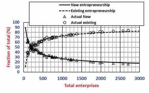
The fraction (%) that new and existing entrepreneurs constitute of total enterprise numbers at different county sizes are depicted in Figure 1. Actual data (triangles and circles) agree closely with lines developed from the enterprise richness-enterprise numbers power law (Table 4). In Alabama counties with fewer than 200 total enterprises, there is a greater need for additional new entrepreneurs than existing entrepreneurs. At about 200 total enterprises, the needs for the two entrepreneurial types are similar. Beyond 200 enterprises, more existing than new entrepreneurs are needed. At about 2500 enterprises the ratio of existing entrepreneurs to new entrepreneurs reaches a pareto 80:20 value. Figure 1 indicates that economic development and job growth in Alabama counties always require some entrepreneurs who can “sense” business opportunities of types not present in the county. Small counties disproportionately have fewer paid employees, fewer enterprises, fewer highly educated people and lower total GDPs and payrolls (Table 2). In addition, they have disproportionately more poor people and households, and a lower enterprise richness. Their poverty rates are higher as indicated by their enterprise dependency indices (Table 2). Under these conditions, the challenge to stimulate “new” entrepreneurship in small counties could be a daunting challenge. A lack of role models could be an impediment.

Figure 1. The requirement for new and existing entrepreneurial types in Alabama counties of different sizes (measured as total enterprise numbers). Triangles (new entrepreneurs) and circles (existing entrepreneurs) represent actual entrepreneurial activities in the counties.

3.2.2. “New” entrepreneurship and job creation

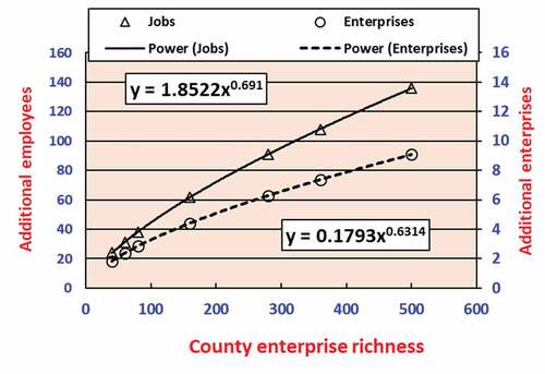
The potential impacts of an additional new enterprise type on enterprise numbers (circles) and employment (triangles) in Alabama counties of different sizes are depicted in Figure 2. These impacts are described by two power laws that indicate that job creation increases at a slightly faster rate than enterprise numbers (Figure 2). The successful founding of a new business type in larger counties is associated with as many as nine additional enterprises and 140 additional jobs, which echoes the findings of Moretti (2013, p. 57). Clearly, increasing the enterprise richness of counties seems to offer a way to stimulate enterprise growth and job creation. This would reduce poverty and distress.

Figure 2. The potential impact of a single additional enterprise type on additional enterprises (circles) and additional jobs (triangles) in Alabama counties of different sizes. Power laws were used to calculate the values.

3.2.3. Poverty, employment and higher education in Alabama counties

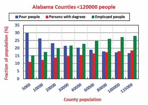
The fraction that poor people, employed people and highly educated persons constitute of the Alabama county populations of different sizes are depicted in Figure 3. Decreases in poverty, and increases in the levels of employment and higher education are associated with increasing county populations. In Alabama, the number of poor people is super-linearly associated with smaller counties. The opposite is the case for the numbers of highly educated persons and employed people.

Figure 3. The levels of poverty, unemployment and higher education in relation to the population sizes of Alabama counties. Power laws were used to calculate values, which were then expressed as percentages of the total population. 

3.2.4. Gross domestic product (GDP), payrolls and total income of Alabama counties

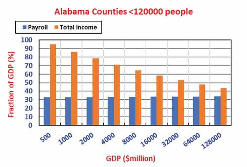
Total county income and county payrolls relative to county GDPs are presented in Figure 4. In counties with small GDPs, total income can approach 90% of GDP whilst payrolls are only about 30%. Income sources other than payrolls, must be important. In large counties, the income to GDP ratio falls to below 50%. In relation to GDP, payrolls are a very constant fraction (~33%) and increase by only approximately one percentage point between small and large counties. As the size of counties increases, an increasing fraction of GDP does not end up in payrolls.

Figure 4. The total income of and payrolls in Alabama counties relative to the magnitude of their gross domestic products (GDPs). Power laws were used to calculate values, which were then expressed as fractions.

These examples illustrate the many challenges of small counties. The stimulatory potential of increasing enterprise richness in terms of issues such as job creation is quantified.

4. Discussion and conclusions

The first impression gained from this contribution is the overall orderliness in the demographic-socioeconomic-entrepreneurial nexus of the selected Alabama counties. Such orderliness has also been reported in regional studies of a group of U.S. counties (D.F. Toerien, 2018) and in the towns of a biosphere reserve in South Africa (D.F. Toerien, 2019).

The second impression gained from this contribution is that most of the studied characteristics of the Alabama counties have similar variation patterns, resulting in statistically significant correlations between them (Tables 2 to 10). The relationships are, however, seldom linear. In other words, two socioeconomic characteristics do not increase or decrease in lock-step. Most of the orderliness is distinctly non-linear, similar to what has been observed in cities (West, 2017). Some characteristics agglomerate disproportionately at lower levels of other characteristics, and others agglomerate disproportionately at higher levels of other characteristics.

An essential feature of all cities is that social activity and economic productivity are systemically enhanced by increasing populations (West, 2017: location 414). Human settlements such as cities obey simple non-linear scaling laws (L.M.A. Bettencourt et al., 2010, p. 2). They are more than the linear sum of their individual components (L.M.A. Bettencourt et al., 2010, p. 1). Socioeconomic scaling occurs in human settlements with urban as well as rural populations. Examples are towns of a South African biosphere reserve (D.F. Toerien, 2019) and Alabama counties (Tables 2 to 10). The disproportionate agglomeration of socioeconomic characteristics is a predominant property of human settlements.

Investigations of distressed communities usually include population estimates (e.g., Department of Community Affairs, 2017; Economic Innovation Group, 2018a; Nunn et al., 2018). Table 2 indicates that larger populations in Alabama counties are disproportionately associated with more paid employees, more enterprises and more highly educated persons. Larger counties are disproportionately associated with fewer poor people and fewer households. Larger populations also are associated with disproportionately larger GDPs, payrolls and total incomes. These are all factors that could reduce distress in communities. Living in larger, rather than smaller counties, seems preferable. The consolidation of some small counties could perhaps help to relieve distress. Table 2 enables quantitative predictions about the impacts of population growth or reduction on a number of socioeconomic characteristics of Alabama counties.

Because of agglomeration phenomena, per capita measures of community wellbeing have to be used with caution (Youn et al., 2016). Table 2 indicates that GDP scales strongly and super-linearly with population. A GDP per capita comparison of more populous Alabama counties with less populous ones would, therefore, in a sense be comparing apples and oranges. In addition, scaling phenomena in regional studies should be considered not only from a population-based perspective but also by considering scaling associated with other socioeconomic characteristics. L.M.A. Bettencourt et al. (2010, p. 7) remarked: “It is therefore extraordinary that, despite the immense diversity of human and social behavior, the dynamics and organization of urban systems, as well as of individual cities, is an emergent predictable phenomenon.” Predictive abilities about Alabama counties have been enhanced by considering scaling phenomena (Tables 2 to 10).

Poverty is central to concerns about distressed communities in the U.S. (Department of Community Affairs, 2017; Economic Innovation Group, 2018a; Nunn et al., 2018; Schanzenbach et al., 2016) and also in Alabama (Scott, 202). Evidence is provided here that six of the socioeconomic characteristics of the selected Alabama counties agglomerate disproportionately in association with increases in the number of officially poor people (Table 9). Poverty in U.S. communities is mostly indicated as a proportion of populations, e.g., as a percentage in the QuickFacts of the U.S. Census Bureau (U.S Census Bureau, 2019), and not in terms of the number of poor people in communities. Because the numbers of populations, paid employees, enterprises and highly educated persons, and the magnitudes of payrolls, GDPs and total incomes of counties, agglomerate disproportionately with increases in the number of poor people (Table 9), it is clear that scaling of socioeconomic characteristics relative to the numbers of poor people, should also be considered when distressed communities are considered.

Scaling impacts associated with regional enterprise numbers have not been reported previously (Table 3). Alabama counties with higher enterprise numbers have disproportionately more highly educated people, higher total incomes and smaller populations. They also have disproportionately fewer poor people and households. Successful entrepreneurship leading to additional viable enterprises should, therefore, enhance the enterprise numbers of Alabama counties and reduce distress.

The mechanisms by which diversity arises and is sustained in complex systems have elicited much research (L.M.A. Bettencourt et al., 2014). Heterogeneity may confer collectives such as communities with the ability (i.e., resilience) to handle selective shocks through a hedging effect that allows some components of the system to survive in times of crisis. The capacity to generate open-ended diversity is one of the most important characteristics of many complex systems, from ecosystems to modern human societies (Youn et al., 2016). This study illustrates that regions are also platforms for studying open-ended economic diversity because regions are also defined socioeconomic units spanning a broad range of scales.

The production of new ideas and the stimulation of socioeconomic development happen largely in urban environments, particularly in large cities (West, 2017). Empirically, diversity has remained difficult to characterize unambiguously. However, this contribution has also shown that enterprise diversity (enterprise richness) can be measured accurately in smaller human settlements, including smaller U.S. counties (Table 4).

Enterprise richness is strongly associated with scaling impacts related to entrepreneurial development in Alabama counties (Table 4). The roles of two broad types of entrepreneurs, i.e., “new” and “existing” entrepreneurs were quantified (Figure 1). With regard to job creation, Moretti (2013, p. 56) focused on two sectors, i.e., the traded and non-traded sectors. He stated that the vast majority of jobs in a modern society are in local services, e.g., people that work as waiters, plumbers, nurses, teachers, etc. These enterprises offer services that are produced and consumed locally, or in other words, in the non-traded sector. Figure 1 suggests that this sector is mainly served by existing entrepreneurs. However, the traded sector is the source of prosperity in U.S. cities (Moretti, 2013, p. 57). In the Alabama counties, this sector probably relates to “new” entrepreneurs (Figure 1) and is associated with the ability to conceive business opportunities that are not yet present in the counties.

Enterprise richness has been related to the knowledge of how to do things, i.e., productive knowledge (e.g., D.F. Toerien, 2018, 2019). The differential accumulation of productive knowledge distinguishes between rich and poor countries and their differences are expressed in the diversity and sophistication of the things that each makes (Hausmann et al., 2017). They added that the productive knowledge to create new products or services is key to economic success and wealth. It is more than book knowledge or searches on the Internet. It is embedded in brains and human networks and is tacit and hard to transmit and acquire. It comes more from years of experience than from years of schooling. Nunn et al. (2018) found that places with higher levels of human capital, more diverse economies, lower exposure to manufacturing, higher population density, and more innovative activity in 1980 tended to have higher vitality scores in 2016, 36 years later. These findings support the views of Hausmann et al. (2017).

Assuming that the views of Hausmann et al. (2017) about the economic fate of countries also apply to regions such as Alabama, enhancing “new” entrepreneurship could be a major factor in dealing with distressed Alabama communities. The ability to measure and use enterprise richness as a proxy for productive knowledge and the power laws reported in Table 4, provide significant predictive capabilities. For instance, Figure 2 illustrates the potential impacts of increases in enterprise richness (i.e., in productive knowledge) on entrepreneurial success and job creation in Alabama counties. These predictions are in step with the views of Moretti about the employment impacts of the production of tradable products (Moretti, 2013, pp. 56–57).

Research in the last couple of decades has shown that education and poverty are inversely related: the higher the level of education of the population, the lower the proportion of poor people in the total population (Tilak, 2001). This was also observed in this study (Table 6). However, no characteristic is super-linearly associated with increases in the number of highly educated people (Table 6). Instead, the number of people, enterprises, poor people and houses, and the magnitude of county GDPs, total income and enterprise richness all scale sub-linearly compared the number of highly educated persons (Table 6). This indicates disproportionate agglomeration of the former characteristics in Alabama counties with fewer highly educated people. This is in step with observations that in a U.S. economy that has grown evermore dependent on knowledge, distressed communities represent the only cohort in which the majority of adults lack an education beyond high school (Economic Innovation Group, 2017).

The respective power laws (Table 2) were used to calculate the population fractions of highly educated, poor people and employed people in relation to county populations (Figure 3). The fraction of poor people decreases as the fractions of highly educated persons and employment increase. The results quantitatively support the contention of Tilak (2001) that fewer poor people in populations are associated with higher levels of education. With regard to distressed communities in Alabama, the challenge obviously is to increase the number of highly educated people, either through attraction of such persons to these communities or by means of enhanced education.

Total county payrolls and the total number of enterprise (paid) employees scale almost linearly in relation to GDP (Table 5). The level of value addition (measured by GDP) is probably an important driver of the number of paid employees and the payrolls in the counties. The numbers of total population, poor people and households, and total county incomes scale sub-linearly relative to GDP (Table 5). Disproportionately lower levels of these characteristics are associated with higher GDPs in Alabama counties. Growth of the GDPs of Alabama counties should be beneficial to distressed communities and Table 5 provides an ability to predict the probable outcomes of such actions.

The scaling of characteristics based on numbers or magnitudes has so far been considered. The enterprise dependency index is not based on numbers or magnitudes but is a ratio. It is a measure of the wealth/poverty states of communities. The higher the index, the more people are needed to “carry” the average enterprise, and vice versa. The power law correlations between enterprise dependency indices and other socioeconomic characteristics in Alabama counties are fairly weak (Table 10) but nevertheless statistically significant (P < 0.01). Such power laws have not been reported before. The power laws have negative coefficients. The implication is that poverty is more prevalent in smaller counties where the values or magnitudes of socioeconomic characteristics are lower. This is another indication that distress is probably disproportionately lower in larger compared to smaller counties.

There is no longer much excuse to ignore many of the measurable properties of cities (Bettencourt, 2013b, p. 5). Cities have many interdependent facets and are social, economic, infrastructural, and spatial complex systems that exist in similar but changing forms over a huge range of scales (Bettencourt, 2013a, p. 1438). Cities realize certain spatial economies of scale as they grow and, simultaneously, attain general socioeconomic productivity gains (Bettencourt, 2013b, pp. 5–6). Comparison of two cities of different population sizes in the same urban system shows that the larger is a little bit denser, and its volume of infrastructure networks per capita (roads, pipes, cables) is smaller. The larger city is usually wealthier, more expensive and more productive technologically. Larger cities are more congested and expensive, but also more exciting culturally. Counties, despite having a rural population component, seem to behave in the same way. So, cities and counties are not just collections of people. They are agglomerations of social links. How do the counties of the case study compare?

The Alabama counties also have many interdependent social and economic facets and are complex systems over a huge range of scales (Tables 1–10). Two examples are used to illustrate this. Firstly, a comparison of two counties of different population sizes shows that the larger county has disproportionately more paid employees, more enterprises, more highly educated persons, larger GDPs, larger payrolls and higher total incomes (Table 2). However, the larger county also has disproportionately fewer households, fewer poor people and a lower enterprise richness. Secondly, a comparison of two Alabama counties on the basis of their poverty states shows that the poorer county has disproportionately fewer people, fewer paid employees, fewer enterprises, fewer highly educated persons, lower payrolls, lower GDPs, lower total incomes but higher enterprise richness (Table 6). This is in step with higher ratios of enterprise richness relative to the total number of enterprises predicted by Figure 1 for smaller counties.

The third, and final, impression of this contribution is that it is possible to view the socioeconomic dynamics of human settlements in a region through a series of different lenses. Here population size (Table 2), the number of enterprises (Table 3), enterprise richness (Table 4), GDP (Table 5), the number of highly educated persons (Table 6), the magnitude of payrolls (Table 7), total incomes (Table 8), the number of poor people (Table 9) and enterprise dependency indices (Table 10) were used. Each lens: (i) provided a separate way to consider the selected Alabama counties, (ii) generated additional insight into the demographic-socioeconomic-entrepreneurial dynamics of human settlements in Alabama, and (iii) delivered significant predictive capabilities.

This is the first analysis of non-linear relationships of a number of socioeconomic and entrepreneurial relationships of counties in a single U.S. state. To expand understanding, counties of other states and other regions require additional analyses of this kind. The list of demographic, socioeconomic and entrepreneurial characteristics that should be analysed could also be expanded. For instance, there is a question if the relationships of different population groups are similar or not.

The fact that so many different characteristics of the selected Alabama counties are closely associated with each other (Tables 2 to 10) makes it inevitable that questions of causality will arise. What-drives-what questions will have to be answered in order to deepen the understanding the demographic-socioeconomic-entrepreneurial dynamics of counties and other regions. Application of the “new science of causal inference” (Pearl & Mackenzie, 2018, p. 1) will probably have to be used in a quest to find answers. Pearl and Mackenzie (2018, p. 2) stated “Yet, until very recently, science gave us no means even to articulate, let alone answer them [cause-and-effect questions]. By far the most important contribution of causal inference to mankind has been to turn this scientific neglect into a thing of the past.” Regions such as U.S. counties about which there are extensive datasets offer exciting research possibilities to further explore the intricacies of their demographic-socioeconomic-entrepreneurial nexus.

Additional information

Funding

The author received no direct funding for this research.

Notes on contributors

Danie Francois Toerien

Research on the demographic-socioeconomic-entrepreneurial nexus of human settlements in South Africa and the United States has been continued over the past few years. Scaling studies were enabled by publicly available datasets in the United States of different characteristics of the nexus. These studies have added to the growing body of knowledge about the extraordinary orderliness of this nexus. The present contribution is based on a case study of Alabama counties. It illustrates that different demographic, socioeconomic and entrepreneurial characteristics can serve as ‘lenses’ to observe human settlements in regional studies. Such analyses can provide deeper insight into problems such as the regression of small towns and the location and dynamics of regional poverty.

References

- Auburn University. (2020). 2020 Alabama State economic report. Government and Economic Development Institute, Auburn University. Retrieved from https://www.auburn.edu/outreach/gedi/documents/2020_AlabamaStateEconomicReport.pdf
- Ball, P. (2005). Critical mass: How one thing leads to another. Randomhouse.
- Beinhocker, E. D. (2006). The origin of wealth: Evolution, complexity, and the radical remaking of economics. Harvard Business School.
- Bettencourt, L., & West, G. (2010). A unified theory of urban living. Nature, 467(7318), 912–29. https://doi.org/10.1038/467912a
- Bettencourt, L. M. A. (2013). The origins of scaling in cities. Science, 340(6139), 1438–1441. https://doi.org/10.1126/science.1235823
- Bettencourt, L. M. A., Lobo, J., Helbing, D., Kühnert, C., & West, G. B. (2007a). Growth, innovation, scaling, and the pace of life in cities. Proceedings of the National Academy of Sciences, 104(17), 7301–7306. https://doi.org/10.1073/pnas.0610172104
- Bettencourt, L. M. A., Lobo, J., & Strumsky, D. (2007b). Invention in the city: Increasing returns to patenting as a scaling function of metropolitan size. Research Policy, 36(1), 107–120. https://doi.org/10.1016/j.respol.2006.09.026
- Bettencourt, L. M. A., Lobo, J., Strumsky, D., & West, G. B. (2010). Urban scaling and its deviations: Revealing the structure of wealth, innovation and crime across cities. Plos One, 5, e13541. https://doi.org/10.1371/journal.pone.0013541
- Bettencourt, L. M. A., Samaniego, H., & Youn, H. (2014). Professional diversity and the productivity of cities. Scientific Reports, 4, 5393. https://doi.org/10.1038/srep05393
- Chen, X., & Roberts, K. A. (2008). Roadless areas and biodiversity: A case study in Alabama, USA. Biodiversity and Conservation, 17(8), 2013–2022. https://doi.org/10.1007/510531-008-9351-2
- Department of Community Affairs. (2017). Measuring distress in New Jersey: The 2017 municipal revitalization index. Office of Policy and Regulatory Affairs, New Jersey Department of Community.
- Economic Innovation Group. (2016). The 2016 distressed communities index. Washington: Economic Innovation Group. Retrieved 24 December, 2018, from https://eig.org/wp-content/uploads/2016/02/2016-Distressed-Communities-Index-Report.pdf
- Economic Innovation Group. (2017). The 2017 Distressed Communities Index. Washington: Economic Innovation Group. Retrieved 24 December, 2018, from https://eig.org/wp-content/uploads/2017/09/2017-Distressed-Communities-Index.pdf
- Economic Innovation Group. (2018a). About us. Washington: Economic Innovation Group. Retrieved 24 December, 2018, from https://eig.org/about-us
- Economic Innovation Group. (2018b). From great recession to great reshuffling: Charting a decade of change across American communities. Distressed communities index October 2018. Washington: Economic Innovation Group. Retrieved 24 December, 2018, from https://eig.org/wp-content/uploads/2018/10/2018-DCI.pdf
- Fujita, M., & Thisse, J. (2002). Economics of agglomeration cities, industrial location, and regional growth. Cambridge University Press.
- Gardiner, B., Martin, R., & Tyler, P. (2010). Does spatial agglomeration increase national growth? Some evidence from Europe. Journal of Economic Geography,11, (6), 979–1006. https://doi.org/10.1093/jeg/lbq047
- Glaeser, E. (2011). Triumph of the city. Penguin.
- Greenstone, M., & Looney, A. (2011). Renewing economically distressed American communities. Issues in Science and Technology, 27(2), 59–67.
- The Hamilton Project. (2018). Overview. Brookings Institute. http://www.hamiltonproject.org/about/
- Hausmann, R., Hidalgo, C. A., Bustos, S., Coscia, M., Chung, S., Jimenez, J., Simoes, A., & Yıldırım, M. A. (2017). The atlas of economic complexity: Mapping paths to prosperity. Center for International Development, Harvard University.
- Kline, P., & Moretti, E. (2014). Local economic development, agglomeration economies, and the Big Push: 100 years of evidence from the Tennessee valley authority. The Quarterly Journal of Economics, 129(1), 275–331. https://doi.org/10.1093/qje/qjt034
- Lobo, J., Bettencourt, L. M. A., Strumsky, D., & West, G. B. (2013). Urban scaling and the production function for cities. Plos One, 8, e58407. https://doi.org/10.1371/journal.pone.0058407
- Magurran, A. (1988). Ecological diversity and its measurement. Crown Helm.
- Markusen, A. (1996). Interaction between regional and industrial policies: Evidence from four countries. International Regional Science Review, 19(1-2), 49–77. https://doi.org/10.1177/016001769601900205
- Mayer-Schönberger, V., & Cukier, K. (2014). Big data: A revolution that will transform how we live, work and think. John Murray Publishers, London.
- Moretti, E. (2013). The new geography of jobs. Mariner Books.
- Nunn, R., Parsons, J., & Shambaugh, J. (2018). The geography of prosperity, report of The Hamilton project. The Brookings Institution.
- Ortman, S. G., Cabaniss, A. H. F., Sturm, J. O., & Bettencourt, L. M. A. (2014). The pre-history of urban scaling. Plos One, 9, e87902. https://doi.org/10.1371/journal.pone.008790
- Ortman, S. G., Cabaniss, A. H. F., Sturm, J. O., & Bettencourt, L. M. A. (2015). Settlement scaling and increasing returns in ancient society. Science Advances, 1(1), e1400066. https://doi.org/10.1126/sciadv.1400066
- Parr, J. B. (2004). Economies of scope and economies of agglomeration: The Goldstein-Gronberg contribution revisited. Annals of Regional Science, 38(1), 1–11. https://doi.org/10.1007/s00168-003-0142-0
- Pearl, J., & Mackenzie, D. (2018). The book of why: The new science of cause and effect. Basic Books.
- Picou, J. S., & Marshall, B. K. (2007). Social impacts of Hurricane Katrina on displaced K-12 students and educational institutions in coastal Alabama counties: Some preliminary observations. Sociological Spectrum, 27(6), 767–780. https://doi.org/10.1080/02732170701534267
- Porter, M. E. (1996). Competitive advantage, agglomeration economies, and regional policy. International Science Review, 19(1–2), 85–94. doi: 10.1177/016001769601900208
- Schanzenbach, D. W., Bauer, L., & Nunn, R. (2016). Who is Poor in the United States? Examining the Characteristics and Workforce Participation of Impoverished Americans. Report of the Brookings Institution. Part of Hamilton Project. Washington: Brookings Institution.
- Scott, K. (2020). 2020 barriers to prosperity data sheet. Alabama Possible. Retrieved from https://alabamapossible.org/2020/05/21/4480/
- Tilak, J. B. G. (2001). Education and poverty. In M. Melin (Ed.), Education – A way out of poverty? New education division documents No. 12 (pp. 12–23). Swedish International Development Cooperation Agency.
- Tilman, D. (1999). The ecological consequences of changes in biodiversity: A search for general principles. Ecology, 80(5), 1455–1474).
- Toerien, D. F. (2014). ʼn Eeu van orde in sakeondernemings in dorpe van die Oos-Kaapse Karoo (in Afrikaans). LitNet Akademies, 11(1), 330–371.
- Toerien, D. F. (2018). Productive knowledge, scaling, enterprise richness and poverty in a group of small U.S. counties. Cogent Social Sciences, 4(1), 1-18. 1560883. https://doi.org/10.1080/23311886.2018.1560883
- Toerien, D. F. (2019). The demographic-socioeconomic-entrepreneurial nexus of towns in a South African biosphere reserve. In J. A. Daniels (Ed.), Advances in Environmental Research (Vol. 67, pp. 171–224). New York: Nova Science Publishers.
- Toerien, D. F., & Seaman, M. T. (2012a). Proportionality in enterprise development of South African towns. South African Journal of Science, 108(5/6), 38–47. https://doi.org/10.4102/sajs.v108i5/6.588
- Toerien, D. F., & Seaman, M. T. (2012b). Regional order in the enterprise structures of selected Eastern Cape Karoo towns. South African Geographic Journal, 94(2), 137-151. http://dx.doi.org/10.1080/03736245.2012.742782
- Toerien, D. F., & Seaman, M. T. (2014). Enterprise richness as an important characteristic of South African towns. South African Journal of Science, 110(11/12), 9. http://dx.doi.org/10.1590/sajs.2014/20140018
- U.S Census Bureau. (2019). QuickFacts. U.S. Census Bureau. Retrieved from https://www.census.gov/quickfacts
- U.S. Bureau of Economic Affairs. (2018). GDP by county. U.S. Bureau of Economic Affairs. Retrieved December 13, 2018, from https://www.bea.gov/data/gdp/gdp-county
- U.S. Census Bureau. (2018). County business patterns (CBP). U.S. Census Burreau. Retrieved June 23, 2018 from www.census.gov/programs-surveys/cbp/data/datasets.html
- United States. (2017). North American industry classification system. Executive Office of The President.
- West, G. (2017). Scale: The universal laws of life and death in organisms, cities and companies. Weidenfeld & Nicolson.
- Youn, H., Bettencourt, L. M. A., Lobo, J., Strumsky, D., Samaniego, H., & West, G. B. (2016). Scaling and universality in urban economic diversification. Journal of the Royal Society Interface, 13, 20150937. https://doi.org/10.1098/rsif.2015.0937