Rural Livelihoods Diversification in Ethiopia: Evidence of Households around Lake Tana

Abstract

Rural households in Ethiopia are characterized by subsistence agriculture, while empirical evidence reveals that rural livelihoods are limited. The aim of this study was to assess the rural livelihoods diversification with evidence of households surrounding Lake Tana. Data was collected using a survey from 413 households. The results of the study revealed that the mean overall asset score of the households was 0.313. Crop production, livestock rearing and employment were the major livelihood strategies. The households practiced a mean of three livelihood strategies, and the evenness score of the households was 0.18 referring to the dominance of small livelihood strategies. The mean annual income of the households was 26,696 ETB which was found to have a strong positive correlation with the asset possession of the households (r = 0.56). In addition, the Simpson diversification index result showed that 46.3%, 43.8% and 9.9% of households were low, medium and high-income diversifiers, respectively. Diversification groups have shown a significant difference in asset holdings but not in the income of the households. Moreover, significant variations were observed between Tana Zuria Rice and Tana Zuria livelihood zone households in asset, number of strategies, income and diversification status. The study concludes that the asset ownership of the households is limited. Development of rural livelihood assets is recommended to improve rural livelihoods and, as a result, household income.

Keywords:

• Assets
• income
• diversification
• lake tana
• livelihood strategies

Public Interest Statement

Subsistence agriculture characterizes Ethiopian rural households, whereas actual research shows that rural livelihoods are limited. The general objective of the study was to analyze the livelihood assets, strategies and diversification of rural households around Lake Tana of Ethiopia. A total of 10 livelihoods were practiced by the households. Crop farming, livestock keeping, and employment were the main sources of income. The study finds out the limited asset position of households. Around half of the households were low diversifiers. The study suggests asset-building initiatives to boost asset possession and income among rural households in the study area.

1. Introduction

Rural development policies and interventions shall be designed in recognition of background factors and livelihoods variation in each target area. A livelihood comprises the capabilities, assets and activities required for a means of living (Chambers & Conway, 1991). Households can pursue a single or a combination of economic activities for their living. Sustainable livelihoods approach acknowledges that rural households can employ more than one livelihood strategy sequentially or in parallel for the sake of the livelihood outcomes. This means that rural farmers may engage in various on-farm, non-farm and off-farm sources (Erenstein et al., 2007). As more livelihood assets are available to the household, there will be a great chance to practice varied livelihood strategies by the households (WFP, 2009). A high number of poor people covering 70–75% of the total poor reside in rural areas of the world depending on agricultural activities (Erenstein et al., 2007). In the same way, the vast majority of the people in the Horn of Africa rely on agriculture as a means of a living (FAO, 2020).

In Ethiopia majority of the people are rural dwellers (. Although rural livelihoods in Ethiopia are endangered by a lack of assets among other factors, their contribution to the households and the country is enormous (Belay & Bewket, 2015). Agriculture is the principal source of food and income in Ethiopia that employs about 75–85% of the population (Bachewe et al., 2019; CDRC, 2019; Diriba, 2020; FAO, 2020). The sector contributes to 34–40% of the total GDP and 79–80% of export trade that delivers 27.5 billion dollars for the country (Admassu et al., 2013; Bachewe et al., 2019; Diriba, 2020). Besides agricultural activities, people pursue other livelihood strategies in response to diverse push and pull factors. In many developing countries, diversification of rural livelihood strategies is found to be an important income making sources (Yona & Mathewos, 2017). Even though agriculture is a prominent strategy in Ethiopia, people diversify on-farm, off-farm and non-farm strategies (Kassa, 2019). Rural households in Ethiopia engaged in off-farm and on-farm livelihood strategies to cope with the varied shocks happening to the community and their livelihoods (Gebru et al., 2018). According to Robaa and Tolossa (2016) off-farm and non-farm livelihood strategies are used as a supplementary income means for the rural households.

The issue of livelihoods is a center of focus in rural poverty reduction efforts of developing countries including Ethiopia (Ellis, 2000). In recognition of that, numerous studies were conducted on rural livelihoods in different corners of Ethiopia. Bazezew et al. (2013) analyze the rural households’ livelihood assets, strategies and outcomes in drought-prone areas of the Amhara region. In addition, Eneyew and Bekele (2012), Eneyew (2012), and Gebru et al. (2018) find out the determinants of livelihood diversification in pastoral societies in southern Ethiopia and Tigray region. Moreover, Yona and Mathewos (2017) analyze the challenges of livelihood diversification in Sidama zone.

Local livelihoods knowledge is relevant for designing suitable development policies and interventions as well as for setting a baseline for monitoring and evaluation of interventions impacts. Consequently, analysis of livelihoods shall be a fundamental step in the development of a rural community for both emergency management and long-term development initiatives (Dagar et al., 2021; Dinku, 2018; FEG, 2006; Islam et al., 2021; Rehman et al., 2021). Nevertheless, no study is conducted about the livelihood assets, strategies and income diversification of households around Lake Tana. This study was designed to address the potential knowledge gap towards households’ livelihoods settled around Lake Tana. Hence, the objective of the study was to analyze the livelihood assets, strategies and diversification in rural areas around Lake Tana of Ethiopia. The study is one of its kind in its comparative analysis of the two livelihood zones: Tana Zuria Rice Livelihood Zone (TZR) and Tana Zuria Livelihood Zone (TZA).

2. Description of the study area

The study area, Lake Tana, is a tropical lake situated in the north-western part of Ethiopian highlands (Mundt, 2011; Tewabe, 2015; Vijverberg et al., 2009). Lake Tana is around 563 km away from Addis Ababa which is the capital city of Ethiopia (UNESCO, 2015). Administratively, the lake is found in the Amhara National Regional State (ANRS) of Ethiopia. The absolute location of the lake extends from 11°25ʹ07”–12°29ʹ18” north to 36°54ʹ01”–37°47ʹ20” east (UNESCO, 2015). Lake Tana is the largest lake in the country, and it is found at an altitude of 1830 m above sea level (Mundt, 2011; Vijverberg et al., 2009). The average temperature of the Lake Tana basin is 20°C (Abebe et al., 2017), while the rainfall of the basin extends from 816 up to 2344 mm (ADSWE, 2015). Lake Tana basin is a home for numerous biodiversity resources. The basin delivers a comfortable place for various flora and fauna. Cultural heritages and waterfalls in the Blue Nile basin are well acknowledged and are good sources of the region’s economy (Mundt, 2011). The Lake Tana basin holds an endemic fish species that are unique across the world. Among 27 fish species in the Lake Basin, 20 of them are endemic to the area (Tewabe, 2015).

Like the rest of the country, 88.6% of the population in Amhara National Regional State reside in rural areas and their economy is dependent on subsistence agriculture (ANRS, 2011). As a natural resource, Lake Tana supports the settlement and livelihoods of many people. About 2 million people live near Lake Tana and its catchment including the town of Bahir Dar (Vijverberg et al., 2009). In other information, Ejigu and Ayele (2018) pointed out that Lake Tana and its watershed provide livelihoods security for 5 million people. More specifically, Lake Tana and neighboring wetlands deliver a livelihood for more than 500,000 people both directly and indirectly (Vijverberg et al., 2009). Lake Tana supports various livelihoods, though agriculture is the dominant one (Goshu & Aynalem, 2017). Fishing is the major livelihood of the surrounding people, but today because of different natural and human made calamities these resources are in danger not only the fish resource but also the entire lake is at risk.

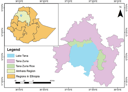
Livelihoods are influenced by locations and resources available in the area that determine opportunities available to the people (Ajala, 2008). Patterns of livelihoods are usually shown in livelihood zone maps, and this is the first step for livelihood-based analysis (FEG, 2006). Livelihood zone is a geographical area at which people engage in the same pattern of livelihoods and access to market (Holzmann, 2008). According to a report generated by USAID (2018) areas around Lake Tana fall under two livelihood zones: Tana Zuria Livelihood Zone (TZA) and Tana Zuria Rice Livelihood Zone (TZR) (Figure 1). The two livelihood zones used to be one primarily and letter on split into two in recognition of the rice production which is a distinctive characteristic for TZR (USAID, 2017).

Figure 1. Location map of Tana Zuria and Tana Zuria rice livelihood zones.

Source: Compiled using ET_LHZ_2018

3. Methodology

Research design: Different research designs can be employed for livelihood study. Considering the objective of this study, explanatory research design based on cross-sectional survey was applied. The household survey was the main data source of the study. In this regard, Moratti and Natali (2012) noted that economic and social situations of households can be best captured by household-based surveys.

Sampling techniques: The household survey was conducted in May 2021 in randomly selected two districts that are adjacent to Lake Tana. Gondar Zuria district was selected representing the TZA and Fogera district representing the context of TZR. Among the total Lake Tana adjacent Rural Kebele¹ Administrations (RKAs) in the two districts, six RKAs (Wegetera, Kideste Hana, Nabega, Furka dangure, Lamba arbayetu insisa and Shehego menge) were randomly selected to gather data for the study. The sample size of this study was determined by using Yamane (1973) formula with 95% confidence level.

$\mathrm{n}=\frac{N}{1+N{\left(e\right)}^2}$

where, n = sample size, N = total population and e = margin of error.

$\frac{105,000}{1+105,000{\left(0.05\right)}^2}=398$

Accordingly, the minimum sample size for the household survey was 398. However, the study has used a sample of 413 households.

The respondent households engaged in the survey were selected through a systematic random sampling technique. Semi-structured questionnaire was a data collection tool for the study.

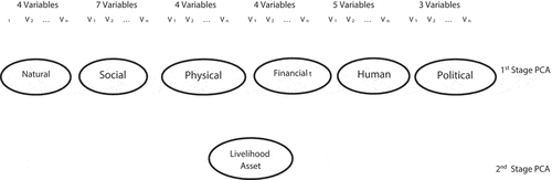
Data analysis techniques: Since the unit of analysis shall be a defined social level in livelihood studies, the level of analysis in this study was determined as household because it is a basic unit at which production, consumption and income generation are conducted (DfID, 1999; FEG, 2006). Data of the study were analyzed using descriptive statistics, principal component analyses (PCA), livelihood asset index, Simpson evenness index and Simpson diversification index (SDI). Two-stage principal component analyses were employed to generate the six livelihood assets indexes and overall asset score of the households. Simpson's evenness and diversification index were applied to check the evenness and income diversification status of rural livelihoods, respectively. The mean score differences of assets, livelihood strategies, income and diversification between TZR and TZA were tested by independent sample t-test. In addition, one-way ANOVA was used to test the asset and income variations across low, medium and high diversification groups. Analyses of the study were conducted employing STATA version 15.0 software. Radar chart was developed to display the assets index using Excel 2010, while ArcGIS 10.4 was applied to generate the maps as shown in the succeeding discussions.

3.1. Livelihood asset index

Livelihood asset index was used to measure the household’s asset possession in the study area. The livelihood asset index was selected due to its strong and internally logical outputs and its development is not conceptually difficult (Filmer & Pritchett, 1998; Kabubo-Mariara et al., 2013). Selection of variables and determination of their weights are two major methodological issues in asset index development. However, the selection of weight approaches has small differences, while variable determination is found with significant impact in empirical studies (Wai-Poi et al., 2008).

There is a wide range of possible household characteristics that could be included in an index (Zakari et al., 2021). Typically, indices will include a number of asset ownership indicators (Wai-Poi et al., 2008). Variables selection should be based on theoretical reflections and previous empirical studies experience. For the sake of this study, variables that were intended to create a livelihood index were selected from previous studies on the issue and theoretical considerations (Table 1). A total of 27 variables from all the classes of the asset types were selected to construct the livelihood indexes. Reciprocal transformation (1/Xi) was applied on some of the variables (distance to road, water sources, and health services) to reconcile the implication of the measurement to the indexes that will be constructed.

Table 1. Description of variables used for livelihood asset index

Asset Type	Variable	Measurement
Physical Asset	Distance to nearest road	Distance in minutes by foot
	Movable asset	Sum of movable assets price in ETB*
	Productive asset	Sum of productive assets price in ETB
	Electricity	0.No 1.Yes
Natural Asset	Land size	Land ownership of the HH in hectare
	Quality of land	1.Infertile 2.Medium 3.Fertile
	Irrigated land size	Hectare of irrigated land owned by the HH
	Distance to nearest water source	Distance in minutes by foot
Social Asset	Farmers cooperative	Membership in the social groups 0.No 1.Yes
	Trade or business association
	Iddir/burial society
	Equib/credit or saving group
	Debbo/work group
	School committee
	Health committee
Financial Asset	Livestock ownership	Tropical Livestock Unit (TLU)
	Saving	Amount of cash saved in ETB
	Access to credit	0.No 1.Yes
	Income	Annual income from all sources
Human Asset	Sex of HH head	0.Female 1.Male
	Age of HH head	Age in years
	Distance to nearest school	Distance in minutes by foot
	Distance to nearest health service	Distance in minutes by foot
	Household size	Number of household members
Political Asset	Membership in political party	0.No 1.Yes
	Membership in women/youth association	0.No 1.Yes
	Membership in RKA leadership	0.No 1.Yes
Overall asset	Composite index generated from the six asset types

* = ETB-Ethiopian Birr (Currency of Ethiopia)

Another task in livelihood assets index construction is weight determination of variables. The entry of all variables into multivariate equations was used for this study. This method determines the weights of variables based on the collected data rather than using equal assignment and other sources (Sahn & Stifel, 2003). Diverse approaches including principal component analysis (PCA), factor analysis, multiple correspondence analysis (MCA) and dichotomous hierarchical ordered probit model (DiHOPIT) can be computed to weight the variables selected to construct the asset index (Wai-Poi et al., 2008). Even though principal component analysis and factor analysis are frequently used approaches, principal component analysis was selected to determine weights of variables in this study.

Assets are the most complex elements of a livelihood, and they are of various types: physical, social, financial, natural, human and political (Ibrahim et al., 2017, 2018). A two-stage principal component analysis was employed to derive weights of variables and to construct the livelihood asset index of rural households (Figure 2). Then, the variables from each asset category were used to construct the six asset-type indexes at the first stage. At the second stage of the principal component analysis, the asset indexes were employed as an input to construct the overall livelihood asset index.

Figure 2. Two-stage livelihoods asset index development.

Source: Authors development, 2021

The score of every household was generated from a linearly weighted score of selected asset indicator variables. According to Kabubo-Mariara et al. (2013) and Sahn and Stifel (2003) an asset index is constructed based on the following equation

${\mathbf{A}}_{\mathbf{i}}={\mathbf{Y}}_{\mathbf{1}}{\alpha }_{\mathbf{1}}+\hspace{0.17em}\dots +{\mathbf{Y}}_{\mathbf{k}}{\alpha }_{\mathbf{k}}$

Where A_i is the asset index, the α_k’s are the individual assets recorded in the survey, and the Y_k’s are the weights to be generated from principal component analysis. The livelihood asset holding of the study households was further classified into quintile groups with consideration of previous studies conducted by Filmer and Pritchett (2001), Gwatkin et al. (2007), Alvarado et al. (2021), and Alvarado et al. (2022), and Mmopelwa and Lekobane (2015). Quintiles groups were usual in asset indexes as they enable the assessment of asset status across other variables. The classification cutoff points for the asset index were less than or equal to 0.2 (very low), 0.21–0.4 (low), 0.41–0.6 (Moderate), 0.61–0.8 (high) and above 0.8 (very high).

3.2. Livelihood diversity measures

The study tried to capture the three important elements of livelihood diversification: richness, evenness and diversification. Livelihoods richness (S) is the number of livelihoods in a given area of study. A simple count of livelihood strategy types was done to identify the livelihoods richness of households in the study area.

The Simpson evenness index (E) was used to assess the evenness of livelihood strategies in the study area. Evenness of a livelihood strategies considers the number of livelihood strategies and their relative abundance in the study area (Moore, 2013). According to Krebs et al. (1999) Simpson’s index of evenness is calculated as shown below

${\mathbf{E}}_{1/\mathbf{D}}=\hspace{0.17em}\frac{1/\mathbf{D}}{\mathbf{S}}$

where: E_1/D represent Simpson’s measure of evenness, D Simpson’s index (D =$\sum {\mathrm{P}}_{\mathrm{i}}^2$) indicating the income proportion of livelihood strategies and S the number of livelihood strategies in the study area. The score of the evenness index is between 0 and 1 (Krebs et al., 1999).

Diversity index shows the number of individual elements and the evenness of individual elements in quantitative terms. The value of the diversity index increases when the amount of variety elements increases and the evenness of their distribution increases (Kiernan, 2020). The usual indexes to measure diversification are Herfindahl Index, Simpson Diversity Index, Ogive Index, Margalef’s Index, Shannon Index, Berger-Parker Index and Entropy Index (Adjimoti & Kwadzo, 2018). For this study, Simpson diversification index (SDI) was selected to estimate the livelihood diversification due to its wider applicability and strength (Khatun & Roy, 2012). The unique benefit of the Simpson diversification index is that it does not expect the engagement of households in all of the livelihood activities (Adjimoti & Kwadzo, 2018). The index was developed by statistician Simpson (1949) to assess the species diversity, and letter on it was adopted and frequently employed by livelihood diversification studies.

According to Khatun and Roy (2012) the formula for Simpson's diversification index is as follow

$\mathbf{S}\mathbf{D}\mathbf{I}=1-\sum _{\mathbf{i}=1}^{\mathbf{N}}{\mathbf{P}}_{\mathbf{i}}^2$

where N is the total number of income sources and Pi represents the income proportion of the i^th income source. The output values of the Simpson diversity index are sorted from 0 to 1. The diversity of livelihoods increases as the value of the index approaches 1. A complete specialization is denoted by 0 while a value of 1 represents pure diversity (Khatun & Roy, 2012; Kiernan, 2020). Livelihood diversification score of the households was further classified into low diversifier (less than 0.39), medium diversifier (0.39–0.63) and high diversifier (above 0.63) based on the recommendation of Saha and Bahal (2010).

3.3. Significance of the study

This study forwarded an important clue in filling the information gap on rural livelihoods of households around Lake Tana. Specifically, the results of the study have some contributions and benefits for academicians, policy-makers, implementers and researchers. For academics, it may provide an insight towards the application of principal component analyses (PCA), livelihood asset index, Simpson evenness index and Simpson diversification index (SDI). In addition, the findings of this study can help different governmental and nongovernmental implementer organizations to design and implement livelihoods development measures. Moreover, the study generated first-hand information on rural livelihoods and income diversification in the study area for those who are interested in conducting further research on the issue.

4. Results and discussion

4.1. Livelihood asset estimates

The primary analysis of this study was estimation of the six livelihood assets and the overall livelihood asset indexes. A minimum of three variables were used to estimate the livelihood asset indexes of the rural households. Theoretical considerations and empirical experiences were accredited on the selection of the variables. Before the main analysis, the achievement of the variables on the preconditions of principal component analysis was checked using a factor test for each asset type. The determinant of the correlation matrix was greater than 0.00001, the Bartlett test of sphericity was significant at less than 1% significant level and finally the KMO measure of sampling adequacy was above the minimum, 0.5, for all of the indexes constructed. As a result, the principal component analysis can be conducted since the variables have met all the minimum criteria.

The first component of the principal component analysis was used to estimate the livelihood assets. As a summary of the results in Annex 1 shows, the first components of principal component analysis explained 23–49% of the total commune variance among variables computed to construct the asset indexes. Subsequently, the analysis considered the units of measurement difference among the variables, the normalization was conducted after the indexes were predicted using min-max normalization method and the values of the indexes ranges between 0 and 1. The weights of each variable for the indexes constructed are presented in Annex 1.

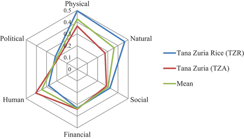
The result of the first stage principal component analysis showed that the entire six livelihood asset types have a small mean score, which was below 0.5 for both TZR and TZA households (see, Table 1). This result implies that households have limited asset holding. The asset holding of the TZR and TZA households showed a significant difference in physical, natural and human asset at less than 1% significant level. At the second stage principal component analysis, the six livelihood asset index scores were used to estimate the overall asset-holding status of the households. The result showed a mean overall asset score of 0.313 with a standard deviation of 0.182 while the TZR and TZA households have 0.346 and 0.284 scores, respectively, which was statistically significant difference at less than 1% significant level.

As Table 2 shows, low asset holding in the study area indicates that the households have low input to run their livelihood strategies. Assets are the cornerstones for the development of people's livelihoods as they are based upon diverse asset types. Livelihood assets determine the capacity of households to practice livelihood strategies. However, the poor asset base of the households in the study area can limit the engagement of the households in diverse livelihood strategies and can lead to unfavorable outcomes from the livelihoods. In addition, livelihood strategies are in favor of more income, food security, sustainable use of natural resources and others. Therefore, lack of assets can lead to unfavorable negative outcomes of livelihood strategies.

Table 2. Summary of livelihood assets index result

Type of asset index	Livelihood Zone				Total (n = 413)		Mean difference	t-test
	Tana Zuria Rice (TZR) (n = 191)		Tana Zuria (TZA) (n = 222)
	Mean	SD	Mean	SD	Mean	SD
Physical	0.495	0.268	0.366	0.239	0.426	0.260	0.129	5.1692***
Natural	0.465	0.199	0.273	0.149	0.362	0.198	0.192	11.1844***
Social	0.321	0.218	0.287	0.189	0.303	0.203	0.033	1.6699
Financial	0.331	0.221	0.340	0.226	0.336	0.011	−0.009	−0.3954
Human	0.279	0.179	0.406	0.210	0.347	0.206	−0.128	−6.5834***
Political	0.214	0.322	0.185	0.301	0.198	0.311	0.029	0.9444
Overall	0.346	0.191	0.284	0.170	0.313	0.182	0.062	3.501***

***P < 0.01

The mean score of the six livelihood asset indexes across the TZR and TZA was displayed by the following radar graph (Figure 3).

Figure 3. The six livelihood asset score of households across livelihood zones.

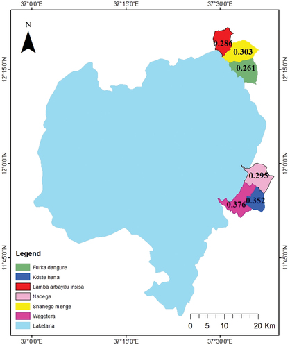
The variation of the overall livelihood asset indexes across the Rural Kebele Administrations (RKAs) was also examined. The three RKAs representing the TZR (Wegetera, Kideste Hana and Nabega) showed higher overall asset possession compared to the TZA sample RKAs (Furka Dangure, Lamba Arbayetu Insisa and Sheheg Menge). The overall asset index score of the study RKAs is displayed in Figure 4.

Figure 4. Overall asset index score of sample RKAs.

Source: Authors production, 2021

After computing the overall asset index score of the households, the data was further classified into quintile groups to observe the distribution of households across the index. Table 3 shows the high livelihood asset index difference across the quintile groups both on the TZR and TZA livelihood zones. The result showed that most of the households were highly distributed at the lowest two asset quintile groups. About 71.9% of the total sample households were grouped under the very low and low asset possession category while only 28.1% of the households possessed assets at moderate, high and very high groups.

Table 3. Livelihood assets quintile across the livelihood zones

Asset quintile group	Livelihood Zone				Total (n = 413)
	Tana Zuria Rice (TZR) (n = 191)		Tana Zuria (TZA) (n = 222)
	Number	Percent	Number	Percent	Number	Percent
Very low	44	23.0	77	34.7	121	29.3
Low	83	43.5	93	41.9	176	42.6
Moderate	40	20.9	41	18.5	81	19.6
High	18	9.4	11	5.0	29	7.0
Very high	6	3.1	0	0.0	6	1.5
Total	191	100	222	100	413	100

4.2. Rural livelihood strategies

The interaction of assets with available policies, institutions and strategies directs the livelihood strategies preference of the rural households. The study tried to capture the richness of the study area in terms of the number of livelihood strategy types. Households’ livelihoods analysis around Lake Tana depicted that there are 10 different types of livelihood strategies practiced by the study sample households. Nevertheless, the sample households have reported their engagement in one up to six livelihood strategies. The result of the study noted that more than half (54.4%) of the households depend on three income sources while 1.2% and 23.1% of the households engaged in one and two livelihood strategies, respectively. An engagement in four and more strategies was achieved by the remaining 21.6% of the households. The mean number of strategies employed by TZR and TZA has shown a significant difference at less than 1% probability level (Table 4). The average number of the livelihood strategies practiced by the households settled around Lake Tana was 3.0. This result was consistent with the work of Gautam and Andersen (2016) which was 2.9 in Humla, Nepal. However, it was lower than (1.86) to the present study that has been reported by Eneyew (2012) in pastoral societies of Southern Ethiopia.

Table 4. Distribution of number of livelihood strategies across the livelihood zones

Number of livelihood strategies practiced	Livelihood Zone				Total (n = 413)
	Tana Zuria Rice (TZR) (n = 191)		Tana Zuria (TZA) (n = 222)
	Number	Percent	Number	Percent	Number	Percent
1	4	2.1	1	0.5	5	1.2
2	63	33.0	32	14.4	95	23.1
6	80	41.9	144	64.9	224	54.4
4	41	21.5	38	17.1	79	19.2
5	3	1.6	4	1.8	7	1.7
6	0	0.0	3	1.4	3	0.7
Total	191	100	222	100	413	100
Mean	2.87		3.09		2.99
t-test	−2.8964***

The significance of the variables is given in the three of the tables. Please have a close look to the tables.

In addition, the combination of livelihood strategies was assessed by the study. Rural households engage in different livelihood strategies available to pursue their living. The livelihood strategies practiced by the households in the study area fall under a combination of diverse livelihood groups: on-farm, non-farm and off-farm. On-farm livelihood group encompasses crop production and livestock rearing (Noronha, 2019). Non-farm livelihood strategies are characterized by being out of the agricultural market system and they are differentiated from on-farm and off-farm by not consuming natural resources (Manjur et al., 2014; Noronha, 2019). In addition, agriculture-related strategies implemented beyond the farm land were considered as off-farm (Noronha, 2019; Yilebes, 2017). Four different combinations of livelihood groups were found practiced by the study area households: On-farm only, on-farm+ off-farm, on-farm+ non-farm and on-farm+ off-farm+ non-farm. The extent of household’s engagement in the livelihood groups showed variation across the two livelihood zones.

Results of the study presented in Figure 5 show that 21.8% of the total households engaged only in on-farm livelihood strategies while the rest of the sample households combined on-farm with other livelihood groups. With regard to the livelihood zones, 33.5% of TZR households practiced only on-farm whereas only 11.7% of TZA households depend on on-farm livelihoods. On-farm was found as the most common and dominant livelihood group in the study area. Consequently, all of the sample households were engaged in at least one of the on-farm livelihood strategies. Similar to this study, an engagement of all households on on-farm strategies was found in Humla, Nepal (Gautam & Andersen, 2016).

Figure 5. Household’s engagement in livelihoods strategies across the livelihood groups.

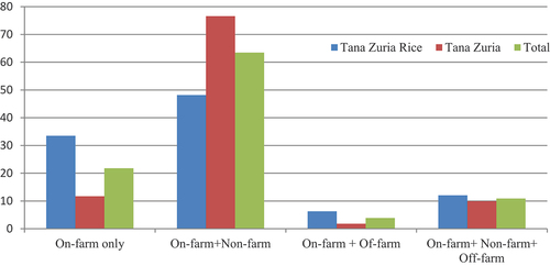
Majority of the respondents (63.4%) employed a combination of on-farm and non-farm livelihood strategies. The engagement of the TZR and TZA households in this livelihood group was 48.2% and 76.6%, respectively. Employment, trade, handicraft, carpentry, service delivery and gifts were the non-farm livelihood strategies in the study area. Employment, which can be permanent or temporary, was found as the third most important strategy in terms of the number of households’ engagement reported by 68% of the study area sample households. The water hyacinth control initiatives around Lake Tana create a window of temporary employment opportunity for the rural households in the area. In addition, a small proportion of sample households are involved in the trade of livestock, food and drink (7.8%), handicraft (0.7%), carpentry (0.7%), service delivery (1%) and gift (12.1%).

On the other side, only 3.87% of the sample households practiced a combination of on-farm and off-farm strategies. The percentage of households in this livelihood category was 6.3% and 1.8% for TZR and TZA households, respectively. The study found 8.2% of fishery production and 6.3% of forest products. Even though the study area is adjacent to Lake Tana, a limited number of people are found engaged in fishery. This is due to the existence of water hyacinth weed on the lake that makes the fishing challenging through reducing the fish stock, damaging the fishing materials, blocking the lake entry points and preventing navigation on the lake.

Finally, 10.9% of the sample households were found depending on the combination of on-farm, non-farm and off-farm strategies. Little variation was observed in the percentage of households implementing the three livelihood groups on TZR and TZA households.

4.3. Income of the rural households

Livelihood strategies are intended to present favorable livelihood outcomes including increased income, improved productivity, food security attainment, poverty alleviation, better conservation of natural resources and many others. Rural households practice livelihood strategies for the sake of different socio-economic outcomes including income. This study also assessed income sources and the extent of income generated from the sources in the study area.

The income sources and the mean annual income earned from the rural households across diverse strategy sources are presented in Table 5. The study indicates that on-farm livelihood sources (mainly crop production) are the major income source of the households. This means that crop production merely contributed for more than half (55.2) of the households income while animal production delivered for 19.8% of the total income. Crop production through the sale of crop and crop products was found to be the primary source with an annual income of 14,724 ETB. Among the total 99.3% of households that practiced crop production in the study area, only 88.6% have generated income from the strategy whereas the rest consumed the outputs for their own consumption. Sale of livestock (cow, sheep, goat and hen) and livestock products (milk, butter, cheese, honey and egg) delivered a mean annual income of 5274 ETB. Similar to the crop production, despite 95.16% of the sample households engaged in livestock production only 49.4% of the households created an income from the strategy. Temporary and permanent employment, trade and gifts appeared as the important income sources of the rural households generating 12 up to 2.3% of the total income share. On the other hand, handicraft, carpentry, service delivery and forestry yielded income that was less than 1% of the total income share. The mean annual income of TZR rural households was 21,069 ETB while TZA households reported 31,538 ETB. The independent sample t-test result disclosed that the mean income difference, 10,469 ETB, between the two livelihood zones was significant at less than 1% probability level.

Table 5. Summary of mean annual income from livelihood strategies in ETB

Source of income	Livelihood Zone						Mean (n = 413)			Income share in Percent
	Tana Zuria Rice (TZR) (n = 191)			Tana Zuria (TZA) (n = 222)
	No	%	Mean income	No	%	Mean income	No	%	Mean income
Fishery	13	6.8	1709	21	9.5	1264	34	8.2	1470	5.5
Crop production	172	90.1	12,723	194	87.4	16,446	366	88.6	14,724	55.2
Livestock production	73	38.2	3756	131	59.0	6580	204	49.4	5274	19.8
Employment	92	48.2	1169	189	85.1	4967	281	68.0	3210	12.0
Trade	14	7.3	570	18	8.1	1164	32	7.7	889	3.3
Handcraft	0	0.0	0	3	1.4	95	3	0.7	51	0.2
Carpentry	0	0.0	63	3	1.4	99	3	0.7	82	0.3
Service delivery	1	0.5	314	3	1.4	59	4	1.0	177	0.7
Forest products	21	11.0	246	5	2.3	170	26	6.3	205	0.8
Gifts	36	18.8	519	14	6.3	695	50	12.1	613	2.3
Total			21,069			31,538			26,696	−2.78***

1USD = 42 ETB

Source: Authors production, 2021

The significance of the variables is given in the three of the tables. Please have a close look to the tables.

In addition, the evenly distribution of the income source livelihood strategies across the two livelihood zones was checked by using the Simpson’s index of evenness. The result showed that the evenness of income sources was found ranging from 0.1 to 0.49, while the mean evenness score of the households was 0.18 with a standard deviation of 0.07. The small evenness score of the study households implies that income from small livelihood strategies dominates the study area. The mean livelihoods evenness score was higher in the TZA households (0.20) compared to what has been recorded in TZR (0.17). The independent sample t-test result confirmed the existence of statistically significant difference in the distribution of livelihood strategies across the two livelihood zone households (t = −4.6917, P < 0.01).

Furthermore, Pearson correlation was conducted to check the relationship between asset possession and annual income of the households. The result indicated that there was strong positive correlation (r = 0.56) between the asset holding and annual income of households. This means the income of the households’ increases with overall asset possession of the households.

4.4. Income diversification of households

Rural households have various means to handle rural threats and the common method is diversification of income sources (Nazir et al., 2018). Income is the main output that households will acquire from livelihoods, and scholars determine the livelihood diversification status of rural households using the income of various sources (Ahmed et al., 2015; Eneyew & Bekele, 2012). Income-based livelihood diversification measurement is highly appreciated due to its clear interpretation (Alobo & Bignebat, 2017). Therefore, this study analyzed the diversification of rural households in consideration of the income share contribution of each strategy in Lake Tan surrounding households.

According to the Simpson diversification index (SDI), the minimum diversification score was found to be zero while the maximum was 0.78. The mean livelihood diversification score of the households was found 0.36 with a standard deviation of 0.23. This result indicates that the mean of the sample households fell under the low diversification status and the households simply focused on limited major types of livelihood strategies. The reason behind low diversification status could be the better agricultural outcomes at the time of normal years that are free from the occurrence of hazards events. The households produce sufficient goods from labor-intensive agricultural practices that lead them to invest most of their resources on agriculture specialization rather than working on diversification of livelihood strategies. The average diversification score of households in this study was smaller than what has been found in Bangladesh (0.42) and western tip pastoral areas of Ethiopia (0.58) estimated using Simpson diversification index (Addisu, 2017; Ahmed et al., 2015).

Taking into consideration the livelihood zones, more than half (57.6%) of the households in TZR are low diversifiers while 36.5% of the households in TZA are found low diversifiers (Table 6). In general, 9.9% of the total households in the study area are high diversifiers whereas 43.8% and 46.3% are medium and low diversifiers, respectively. The mean diversification score for the TZR and TZA households was 0.29 and 0.41 in order of appearance. In addition, the t-test outcome showed the existence of statistically significant difference in the mean SDI score of households between TZR and TZA (t = −5.4113, P < 0.01).

Table 6. Livelihood diversification distribution of households via livelihood zones

Simpson Diversification Index (SDI)	Livelihood Zone				Total (n = 413)		Mean SDI Score
	Tana Zuria Rice (TZR) (n = 191)		Tana Zuria (TZA) (n = 222)
	Number	Percent	Number	Percent	Number	Percent
Low diversifier (<0.38)	110	57.6	81	36.5	191	46.3	0.14
Medium diversifier (0.39–0.63)	67	35.1	114	51.4	181	43.8	0.51
High diversifier (>0.63)	14	7.3	27	12.2	41	9.9	0.67
Total	191	100	222	100.00	413	100	0.36
Mean SDI	0.29		0.41		0.36
t-test	−5.4113***

The significance of the variables is given in the three of the tables. Please have a close look to the tables.

Further analysis was done to assess the relationship between income diversification and asset possession of the rural households in the study area. The result showed that the low-income diversifiers came up with the highest overall asset index score (0.335) while the medium- and high-income diversifiers were found with 0.289 and 0.314 asset-holding status, respectively. The result indicates that households with better asset holding prefer to specialize rather than diversify their income source livelihood strategies.

A one-way ANOVA was conducted to show if the overall asset score within income diversification groups was different for the groups. Participants were classified into three groups: low diversifier (n = 191), medium diversifier (n = 181) and high diversifier (n = 41). Assumptions were checked, and no significant violations were observed. The result showed that there was a statistically significant variation in overall asset possession between the diversification groups at P < 0.05 (F (2,410) = 3.10, p = 0.0461). A post-hoc test using Bonferroni revealed that asset possession was significantly higher in low diversifiers compared to medium diversifiers (0.047, p = 0.040). However, there was no statistically significant difference between low diversification and high diversification (0.022, p = 1.00) and medium diversification and high diversification (0.025, p = 1.00). Similarly, a study conducted by Alobo and Bignebat (2017) has also shown a significant association of income diversification and household asset endowments in rural Senegal and Kenya.

Besides, the mean income difference across the three income diversification groups was checked by the study and an inverse relationship was shown between income diversification groups and income of the households (Table 7 and A1). The low-income diversifiers were found with the highest mean income (27,516 ETB) followed by medium (26,254 ETB) and high (24,828 ETB) income diversifiers. However, the one-way ANOVA test conducted has revealed non-significant differences in annual households income across income diversification groups (F (2,410) = 0.10, p = 0.9017). This finding was in contrast to the result of Eneyew (2012) which has come up with a significant income difference across the income diversification groups in the pastoral societies of southern Ethiopia. By connecting the results, it is possible to infer that low-income diversifiers are characterized by better asset ownership and income and diversification is implemented by low asset owners to support their income.

Table 7. Distribution of asset and income of households on diversification groups

Simpson Diversification Index (SDI)	Mean Overall asset score	Mean income in ETB
Low diversifier	0.335	27,516
Medium diversifier	0.289	26,254
High diversifier	0.314	24,828
Total	0.313	26,696
One way ANOVA (F value)	3.10**	0.10

**P < 0.05

Source: Own survey, 2021

5. Conclusions and the way forward

The study tried to analyze the livelihood assets, strategies and income diversification with an experience of rural households around Lake Tana using the data of 413 sample households selected from six rural kebele administrations (RKAs) in two districts. The rural households in the Lake Tana surrounding areas own poor livelihood asset resources in all of the asset types and overall asset status. TZR households own better assets as compared to TZA and significant differences were observed in asset ownership across the two livelihood zones.

The livelihood strategies richness was found in 10 and the rural households were engaged in one up to six different livelihood strategies. The households implemented an average of 2.99 livelihood strategies and the TZA households implemented a significantly higher number of strategies than TZR households. Crop production, livestock production and employment were the three major types of strategies in the study area in terms of engagement and income generation while all of the sample households implemented on-farm livelihood strategies. Only on-farm strategies were implemented by 21.8% of the household despite the rest employed a combination of strategies: on-farm and off-farm (3.9%), on-farm and non-farm (63.4%), on-farm, non-farm and off-farm (10.9%). The evenness of the livelihood strategies was small due to limited livelihood strategies dominance in the study area.

The rural households generate a mean annual income of 26,696 ETB, while the TZA households have shown a statistically significant higher income as compared to households of TZR livelihood zone. The income of the households was on-farm dominant covering 74.9% of the total income share. The income of the households has a strong positive correlation with the overall asset holding of the households. The study area households employ diverse livelihood strategies to generate income. The income diversification status showed that 46.3% of the households are low diversifiers while 43.8% and 9.9% were medium and high diversifiers. Mean income diversification score of the total households was 0.357 indicating low-income diversification status. The mean income diversification status of the TZR and TRA households was under the low and medium categories with statistically significant differences. Besides, the study concludes that there is a statistically significant difference among asset holdings of the households and income diversification groups. Finally, the study recommends asset-building interventions to enhance asset possession and to increase the income of rural households in the study area.

Availability of data and materials

The dataset supporting the conclusions and recommendations of the study are included in the article.

Consent for publication

The authors provide consent for publication of this manuscript in this journal.

Acknowledgements

The authors acknowledge Bahir Dar University and the University of Gondar for facilitating the study.

Disclosure statement

The authors declare no potential conflcit of interst..

Additional information

Funding

The International Foundation for Science (IFS) I2-W-6666-1 has funded this study. The authors acknowledge the financial support of IFS.

Notes on contributors

Yilebes A. Damtie

Yilebes A. Damtie holds MSc in Disaster Risk Management and Sustainable Development and MSc in Geo-information. He is a PhD candidate in University of Gondar with a specialization in environment and development. He has researched and published 10 research articles in food security, livelihoods and disaster-related issues. Currently, Mr Yilebes is working as an assistant professor in Bahir Dar University, Institute of Disaster Risk Management and Food Security Studies.

Notes

1. Kebele is the lowest administrative level in Ethiopia.

Annex 1

Table A1. Summary of principal component analysis results

Type of Asset	Variable	Scoring coefficients	Proportion	Determinant of the correlation matrix	Bartlett test of sphericity	KMO
Physical Asset	Distance to nearest road	0.03118	0.43	0.691	151.51***	0.552
	Movable asset	0.51663
	Productive asset	0.38769
	Electricity	0.40680
Natural Asset	Land size	0.21525	0.35	0.865	59.66***	0.503
	Quality of land	0.22346
	Irrigated land size	0.80627
	Distance to nearest water source	0.25796
Social Asset	Farmers cooperative	0.45570	0.23	0.728	129.80***	0.584
	Trade or business association	0.32304
	Iddir/ burial society	0.22555
	Membership in Equib/ saving group	0.25642
	Debbo/ work group	0.35190
	School committee	0.21335
	Health committee	0.19517
Financial Asset	Livestock ownership	0.23741	0.43	0.730	128.96***	0.641
	Saving	0.53691
	Access to credit	0.20373
	Income	0.47711
Human Asset	Sex of HH head	0.04858	0.30	0.751	117.30***	0.511
	Age of HH head	0.37821
	Distance to nearest school	0.50242
	Distance to nearest health service	0.50417
	Household size	0.16222
Political Asset	Membership in political party	0.56304	0.49	0.798	92.67***	0.516
	Membership in women/youth associations	0.08095
	Membership in RKA leadership	0.61354
Overall Asset	Physical asset index	0.43738	0.37	0.393	382.46***	0.696
	Natural asset index	0.11391
	Social asset index	0.19365
	Financial asset index	0.40897
	Human asset index	0.03636
	Political asset index	0.25473

Prediction method – Bartlett

References

- Livelihood diversification strategies among men and women rural households: Evidence from two watersheds of Northern Ethiopia (academeresearchjournals.org)Abebe, W. B., Leggesse, E. S., Beyene, B. S., & Nigate, F. (2017). Climate of Lake Tana Basin. In Social and Ecological System Dynamics (pp. 51–22). Springer.
- Addisu, Y. (2017). Livelihood strategies and diversification in western tip pastoral areas of Ethiopia. Pastoralism, 7(1), 1–9. https://doi.org/10.1186/s13570-017-0083-3
- Adjimoti, G. O., & Kwadzo, G. T.-M. (2018). Crop diversification and household food security status: Evidence from rural Benin. Agriculture Food Security, 7(1), 82. https://doi.org/10.1186/s40066-018-0233-x
- Admassu, H., Getinet, M., Thomas, T. S., Waithaka, M., & Kyotalimye, M. (2013). Ethiopia. Chapter, 6, 149–182. https://www.researchgate.net/profile/Michael-Waithaka-2/publication/264724734_Ethiopia/links/53ecb8330cf24f241f159bcd/Ethiopia.pdf
- ADSWE. (2015). Tana sub basin Land Use Planning and Environmental Study Project; Technical Report Volume V: Agro-Climatic Assessment for BoEPLAU (ADSWE, LUPESP/TaSB: 09/2015). Retrieved from Bahir Dar
- Ahmed, M. T., Bhandari, H., Gordoncillo, P. U., Quicoy, C. B., & Carnaje, G. P. (2015). Diversification of rural livelihoods in Bangladesh. Journal of Agricultural Economics Rural Development, 2(2), 32–38 https://www.researchgate.net/profile/Michael-Waithaka-2/publication/264724734_Ethiopia/links/53ecb8330cf24f241f159bcd/Ethiopia.pdf.
- Ajala, O. (2008). Livelihoods Pattern of “Negede Weyto” Community in Lake Tana Shore, Bahir Dar Ethiopia. Ethiopian Journal of Environmental Studies Management, 1(1), 19–30. https://doi.org/10.4314/ejesm.v1i1.41566
- Alobo, S., & Bignebat, C. (2017). Patterns and determinants of household income diversification in rural Senegal and Kenya. Journal of Poverty Alleviation International Development, 8(1), 93–126. https://hal.archives-ouvertes.fr/hal-01608295/
- Alvarado, R., Tillaguango, B., Cuesta, L., Pinzon, S., Alvarado-Lopez, M. R., Işık, C., & Dagar, V. (2022). Biocapacity convergence clubs in Latin America: An analysis of their determining factors using quantile regressions. Environmental Science Pollution Research, 1–17. https://doi.org/10.1007/s11356-022-20567-6
- Alvarado, R., Tillaguango, B., Dagar, V., Ahmad, M., Işık, C., Méndez, P., & Toledo, E. (2021). Ecological footprint, economic complexity and natural resources rents in Latin America: Empirical evidence using quantile regressions. Journal of Cleaner Production, 318, 128585. https://doi.org/10.1016/j.jclepro.2021.128585
- ANRS. (2011). The development study on the improvement of livelihood through integrated watershed management in Amhara region: Final report.
- Bachewe, F. N., Berhane, G., Minten, B., & Taffesse, A. S. (2019). Agricultural growth in Ethiopia (2004-2014): Evidence and drivers, Working paper 81. Gates Open Res, 3(661), 661.
- Bazezew, A., Bewket, W., & Nicolau, M. (2013). Rural households livelihood assets, strategies and outcomes in drought-prone areas of the Amhara Region, Ethiopia: Case Study in Lay Gaint District. African Journal of Agricultural Research, 8(46), 5716–5727. https://doi.org/10.5897/AJAR2013.7747
- Belay, M., & Bewket, W. (2015). Enhancing rural livelihoods through sustainable land and water management in northwest Ethiopia. Geography, Environment, Sustainability, 8(2), 79–100. https://doi.org/10.24057/2071-9388-2015-8-2-79-100
- CDRC. (2019). Poverty and hunger strategic review, Ethiopia’s roadmap to achieve zero poverty and hunger, main report.
- Chambers, R., & Conway, G. (1991). Sustainable rural livelihoods: Practical concepts for the 21st century. Institute of Development Studies (UK).
- Dagar, V., Khan, M. K., Alvarado, R., Usman, M., Zakari, A., Rehman, A., Murshed, M., & Tillaguango, B. (2021). Variations in technical efficiency of farmers with distinct land size across agro-climatic zones: Evidence from India. Journal of Cleaner Production, 315, 128109. https://doi.org/10.1016/j.jclepro.2021.128109
- DfID. (1999). Sustainable livelihoods guidance sheets. London: DFID, 445.
- Dinku, A. M. (2018). Determinants of livelihood diversification strategies in Borena pastoralist communities of Oromia regional state, Ethiopia. Agriculture & Food Security, 7(1), 1–8. https://doi.org/10.1186/s40066-018-0192-2
- Diriba, G. (2020). Agricultural and rural transformation in Ethiopia: Obstacles, triggers and reform considerations,Policy Working Paper 01/2020. Ethiopian Economics Association.
- Ejigu, M., & Ayele, B. (2018). Conserving the Lake Tana ecosystem and biodiversity for sustainable livelihoods and Enduring Peace, 2018 world water week.
- Ellis, F. (2000). The determinants of rural livelihood diversification in developing countries. Journal of Agricultural Economics, 51(2), 289–302. https://doi.org/10.1111/j.1477-9552.2000.tb01229.x
- Eneyew, A. (2012). Determinants of livelihood diversification in pastoral societies of southern Ethiopia. Journal of Agriculture Biodiversity Research, 1(3), 43–52.
- Eneyew, A., & Bekele, W. (2012). Determinants of livelihood strategies in Wolaita, southern Ethiopia. Agricultural Research Reviews, 1(5), 153–161.
- Erenstein, O., Hellin, J., & Chandna, P. (2007). Livelihoods, poverty and targeting in the Indo-Gangetic Plains: A spatial mapping approach (9706481567). CIMMYT.
- FAO. (2020). Desert locust crisis, Appeal for rapid response and anticipatory action in the Greater Horn of. FAO (Food and Agriculture Organization).
- FEG. (2006). Guide to Rural Livelihood Zoning. USAID.
- Filmer, D., & Pritchett, L. (1998). Estimating wealth effects without expenditure data—or tears. Paper presented at the Policy Research Working Paper 1980, The World.
- Filmer, D., & Pritchett, L. H. (2001). Estimating wealth effects without expenditure data—or tears: An application to educational enrollments in states of India: Revised. Demography, 38(1), 115–132. https://doi.org/10.1353/dem.2001.0003
- Gautam, Y., & Andersen, P. (2016). Rural livelihood diversification and household well-being: Insights from Humla, Nepal. Journal of Rural Studies, 44, 239–249. https://doi.org/10.1016/j.jrurstud.2016.02.001
- Gebru, G. W., Ichoku, H. E., & Phil-Eze, P. O. (2018). Determinants of livelihood diversification strategies in Eastern Tigray Region of Ethiopia. Agriculture & Food Security, 7(1), 1–9. https://doi.org/10.1186/s40066-018-0214-0
- Goshu, G., & Aynalem, S. (2017). Problem overview of the lake Tana basin. In Social and Ecological System Dynamics (pp. 9–23). Springer.
- Gwatkin, D. R., Rutstein, S., Johnson, K., Suliman, E., Wagstaff, A., & Amouzou, A. (2007). Socio-economic differences in health, nutrition, and population within developing countries, Country reports on HNP and poverty. The World Bank.
- Holzmann, P. (2008). Household Economy Approach, the Bk: A Guide for Programme Planners and Policy-Makers. Save the Children UK.
- Ibrahim, A. Z., Hassan, K., Kamaruddin, R., & Anuar, A. R. (2017). Examining the livelihood assets and sustainable livelihoods among the vulnerability groups in Malaysia. Indian-Pacific Journal of Accounting and Finance, 1(3), 52–63. https://doi.org/10.52962/ipjaf.2017.1.3.17
- Ibrahim, A. Z., Hassan, K. H., Kamaruddin, R., & Anuar, A. R. (2018). The level of livelihood assets ownership among vulnerability group in East Coast of Malaysia. European Journal of Sustainable Development, 7(3), 157. https://doi.org/10.14207/ejsd.2018.v7n3p157
- Islam, M., Khan, M. K., Tareque, M., Jehan, N., & Dagar, V. (2021). Impact of globalization, foreign direct investment, and energy consumption on CO2 emissions in Bangladesh: Does institutional quality matter? Environmental Science Pollution Research, 28(35), 48851–48871. https://doi.org/10.1007/s11356-021-13441-4
- Kabubo-Mariara, J., Araar, A., & Duclos, J.-Y. (2013). Multidimensional poverty and child well-being in Kenya. The Journal of Developing Areas, 47(2), 109–137. https://doi.org/10.1353/jda.2013.0024
- Kassa, W. A. (2019). Determinants and challenges of rural livelihood diversification in Ethiopia: Qualitative review. Journal of Agricultural Extension Rural Development, 11(2), 17–24. https://doi.org/10.5897/JAERD2018.0979
- Khatun, D., & Roy, B. C. (2012). Rural livelihood diversification in West Bengal: Determinants and constraints. Agricultural Economics Research Review, 25(347–2016–16910), 115–124. https://doi.org/10.22004/ag.econ.126049
- Kiernan, D. (2020). Introduction, Simpson’s Index and Shannon-Weiner Index. https://stats.libretexts.org/Bookshelves/Applied_Statistics/Book%3A_Natural_Resources_Biometrics_(Kiernan)/10%3A_Quantitative_Measures_of_Diversity_Site_Similarity_and_Habitat_Suitability/10.01%3A_Introduction%2C__Simpson%E2%80%99s_Index_and_Shannon-Weiner_Index
- Krebs, C. J., Jarvis, E. D., & Pfaff, D. W. (1999). Ecological methodology. 96. (4). 1686–1691. https://doi.org/10.1073/pnas.96.4.1686.
- Manjur, K., Amare, H., HaileMariam, G., & Tekle, L. (2014). Livelihood diversification strategies among men and women rural households: Evidence from two watersheds of Northern Ethiopia. Journal of Agricultural Economics Development, 3(2), 17–25. https://www.academeresearchjournals.org/print.php?id=5368979b4bf7b
- Mmopelwa, D., & Lekobane, K. (2015). Household wealth status in Botswana: An asset based approach. Global J Human-Social Sci: Economics, 20–28. https://globaljournals.org/GJHSS_Volume15/2-Household-Wealth-Status.pdf
- Moore, J. C. (2013). Diversity, taxonomic versus functional.
- Moratti, M., & Natali, L. (2012). Measuring Household Welfare: Short versus long consumption modules, Working Paper 2012-04, UNICEF Office of Research, Florence.
- Mundt, F. (2011). Wetlands around Lake Tana: a landscape and avifaunistic study. Preliminary research finding of a master thesis, Greifswald University, Germany.
- Nazir, A., Li, G., Inayat, S., Iqbal, M., Humayoon, A., & Akhtar, S. (2018). Determinants for income diversification by farm households in Pakistan. The Journal of Animal Plant Sciences, 28(4), 1163–1173. https://www.thejaps.org.pk/docs/v-28-04/27.pdf
- Noronha, T. (2019). Alternative livelihoods working glossary. Produced by mercy corps as part of the SCALE Award. In.
- Rehman, A., Ma, H., Ozturk, I., Murshed, M., & Dagar, V. (2021). The dynamic impacts of CO2 emissions from different sources on Pakistan’s economic progress: A roadmap to sustainable development. Environment, Development Sustainability, 23(12), 17857–17880. https://doi.org/10.1007/s10668-021-01418-9
- Robaa, B., & Tolossa, D. (2016). Rural livelihood diversification and its effects on household food security: A case study at Damota Gale Woreda, Wolayta, Southern Ethiopia. Eastern Africa Social Science Research Review, 32(1), 93–118. https://doi.org/10.1353/eas.2016.0001
- Saha, B., & Bahal, R. (2010). Livelihood diversification pursued by farmers in West Bengal. Indian Research Journal of Extension Education, 10(2), 1–9 https://web.archive.org/web/20190711095320id_/http://www.seea.org.in:80/vol10-2-2010/01.pdf.
- Sahn, D. E., & Stifel, D. (2003). Exploring alternative measures of welfare in the absence of expenditure data. Review of Income and Wealth, 49(4), 463–489. https://doi.org/10.1111/j.0034-6586.2003.00100.x
- Simpson, E. H. (1949). Measurement of diversity. Nature, 163(4148), 688. https://doi.org/10.1038/163688a0
- Tewabe, D. (2015). Preliminary survey of water hyacinth in Lake Tana, Ethiopia. Global Journal of Allergy, 1(1), 013–018. https://doi.org/10.17352/2455-8141.000003
- UNESCO. (2015). Ecological sciences for sustainable development. https://www.unesco.org/new/en/natural-sciences/environment/ecological-sciences/biosphere-reserves/africa/ethiopia/lake-tana/
- USAID. (2017). Ethiopia livelihood baseline: Amhara region:Tana Zuria livelihood zone
- USAID. (2018). Ethiopia- Livelihood zones.
- Vijverberg, J., Sibbing, F. A., & Dejen, E. (2009). Lake Tana: Source of the Blue Nile. In The Nile (pp. 163–192). Springer.
- Wai-Poi, M., Spilerman, S., & Torche, F. (2008). Economic well-being: Concepts and measurement with asset data, Working Paper. New York University.
- WFP. (2009). Emergency food security assessment handbook. World Food Programme.
- Yilebes, A. (2017). Assessment of food security through livelihood strategies, the case of Lare woreda; Gambella National Regional State, Ethiopia. International Journal of Agriculture Biosciences, 6(4), 183–188. https://www.ijagbio.com/pdf-files/volume-6-no-4-2017/183-188.pdf
- Yona, Y., & Mathewos, T. (2017). Assessing challenges of non-farm livelihood diversification in Boricha Woreda, Sidama zone. Journal of Development Agricultural Economics, 9(4), 87–96. https://doi.org/10.5897/JDAE2016.0788
- Zakari, A., Toplak, J., Ibtissem, M., Dagar, V., & Khan, M. K. (2021). Impact of Nigeria’s industrial sector on level of inefficiency for energy consumption: Fisher Ideal index decomposition analysis. Heliyon, 7(5), e06952. https://doi.org/10.1016/j.heliyon.2021.e06952