Managing score heterogeneity between online consumer review websites

Abstract

This paper describes an alternative approach to measuring score heterogeneity between online consumer review websites. This topic is important in tourism management and in the hospitality sector, where it is helpful to be aware of the ratings obtained by services, from information readily available on the website. We approach this issue by considering tests of multiple population means, assuming this question can be viewed as a clustering problem and that all feasible data configurations can be tested using a Bayesian procedure from which the posterior probabilities of each cluster model are computed. The proposed Bayesian model is a useful alternative to frequentist multiple testing methods, which neglect uncertainty regarding other potential configurations. We draw conclusions about the overall score parameter and propose a Bayesian model averaging model for estimation purposes. Finally, the proposed Bayesian framework is illustrated in detail using a real dataset.

Keywords:

• Bayesian analysis
• Bayes factors
• heterogeneity
• hospitality research
• online consumer reviews

1. Introduction

In recent years, increasing numbers of researchers in business, economics, management, social sciences and related disciplines have been using Bayesian statistics in their data analyses, an approach facilitated by the greater computational power now available with which to address the complexity of statistical models. In tourism studies, too, this method has proven beneficial and offering greater flexibility and enables more intuitive interpretations to be made.

Bayesian analysis has been introduced in tourism in the last two decades where many contributions have been made by Assaf and colleagues. As Assaf et al. (2018) pointed out, the Bayesian approach offers several advantages: 1) It allows previous information to be incorporated into the analysis; 2) It is more robust to small sample sizes; 3) It produces more reliable statistics for formal model comparison; 4) It provides a better approximation for managing uncertainty within the models. Topics addressed in their papers include analyses of cost efficiency and estimated business efficiency, using parametric and non-parametric Bayesian stochastic frontier and DEA approaches (Assaf, 2009, 2011, 2012; Assaf & Tsionas, 2015; Assaf et al., 2021), efficiency in the US hotel industry (Assaf & Magnini, 2012), regression and forecasting models (Assaf & Tsionas, 2019, and references therein), and Bayesian methods and structural equation modelling in tourism research (Assaf et al., 2018). An excellent brief review of the recent literature on Bayesian statistics in tourism management can be found in Bianchi and Heo (2021) and references therein.

However, there is only a very limited body of research literature on the use of Bayesian techniques in tourism and hospitality-sector studies related to electronic word-of–mouth (eWOM), an area in which the frequentist approach is much more prevalent. Probably, the recent paper by S´anchez-Franco et al. (2019) is a prelude to the opportunities offered by such Bayesian methods in this area.

With the increasing incorporation of e-commerce into the tourism industry, however, many consumers now base their hotel selections and reservations on the information offered on tourism websites (Peng et al., 2018). The internet (platforms, applications, etc.) is now a major channel for booking accommodation (Buhalis & Law, 2008) and it is important both for customers and for hotel managers to have a good understanding of the rationale underlying travellers’ booking preferences and their propensity to conduct direct online operations; among other benefits, this knowledge could facilitate significant cost reductions for both parties (Lei et al., 2019). In this respect, the use of a single—value rating is often complemented by multi—criteria ratings or text comments, among other resources (Chen et al., 2021; Nilashi et al., 2019; Zhao et al., 2019). Many studies have analysed the sociodemographic and trip—related characteristics of tourists, including Coenders et al. (2016) and Boto-Garc´ıa et al. (2021). In this respect, too, cognitive variables were used by Fong et al. (2017) to predict tourists’ intention to reuse mobile apps for making hotel reservations, while Boto-Garc´ıa et al. (2021) examined the associations among trip features such as travel purpose, distance to origin, duration of stay and booking mode choice, and confirmed the existence of varying preferences among different population groups.

Many tourism and hospitality researchers have studied the use of eWOM. Some have evaluated online consumer reviews (OCR), such as TripAdvisor (Fang et al., 2016) or Booking.com (Mellinas & Martin-Fuentes, 2021; Mellinas et al., 2015, 2016), while others compare review sites (Xiang et al., 2017). Customer reviews reflect their experience of the hospitality sector, which is usually summarised as a subjective numerical value, commonly ranging from 1 to 10. This area is one in which Bayesian statistics can usefully be considered, as the data already represent a subjective decision (Bianchi & Heo, 2021).

Understanding the heterogeneous preferences for hotel choice attributes across different customer segments is an interesting issue in the hospitality context. In this paper, we will show that the Bayesian approach provides a means of addressing the problem of between—OCR heterogeneity in hospitality management. Analyses of this topic must resolve two significant complications in this regard: firstly, the existence of heterogeneity among OCR webs, a variation that could bias parameter estimates. Furthermore, after this heterogeneity has been identified, it is necessary to syncretise the information in order to generate valid estimates of the quantities of interest and to ensure that the analysis incorporates all the uncertainty presented concerning between—OCR variation. The following motivating example is offered to clarify the problem.

1.1. A motivating case study

The Santa Catalina Hotel is an emblematic, five—star (grand luxury) hotel located in the city of Las Palmas de Gran Canaria in the Canary Islands, Spain, which has attracted national and international celebrities since its inauguration in 1890. The hotel has been a landmark throughout the history of Gran Canaria, an island renowned for its white sand and black lava beaches, and was named Best Historical Luxury Hotel in Europe and Best Luxury Cultural Hotel in Southern Europe at the 2019 World Luxury Hotel Awards.

The dataset used in this article was extracted in June 2022 using public data from Booking.com, TripAdvisor.com and Hoteles.com and cover the time period from 1 January to 31 December 2021. Table 1 summarises the scores received by the hotel from each of these OCR websites.

Table 1. Descriptive quantities of the sample distribution for the three OCR websites

OCR website	Mean	Standard deviation	Sample size (number of reviews)
Booking.com	$9.14$	$1.65$	$n_1=419$
TripAdvisor.com	$9.31$	$2.35$	$n_2=206$
Hoteles.com	$9.37$	$1.42$	$n_3=102$

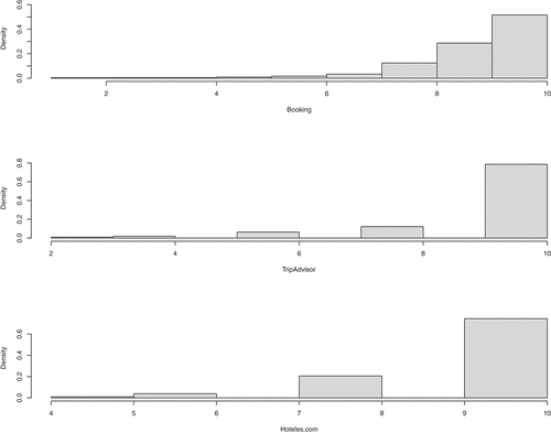
In the present study, our aim is to illustrate how several sources of OCR—scoring information may be aggregated coherently; concerns emerging from different scoring scales are not the subject of this paper (Mellinas et al., 2016). Our analysis uses the standard 1–10 scale, and the TripAdvisor and Hoteles sample data were elementary linear transformed to this conventional scale. Figure 1 shows the histograms for the sample populations.

Figure 1. Feedback histograms for the three OCR websites for hotel Santa Catalina.

The rating information includes summaries of the extent to which reviewers enjoyed a product (scored on a discrete scale ranging from the lowest to the highest possible rating), the number of individuals who have evaluated the product and the average rating of all reviews.

However, when evaluating OCR, concerns may arise regarding the number of individual ratings used to derive an average value; evidently, average ratings that are based on many opinions are more robust information sources than those based on just a few (Hoffart et al., 2019). Therefore, researchers wish to determine the behaviour of the parameter that represents the average ratings, termed $\lambda ,$ to obtain an overall expected score for the OCRs. Also, for each OCR website, ${\lambda }_i$ represents the average ratings obtained from population $i$. In the present case, $i=1,2,3$ represent the OCR websites of Booking, TripAdvisor and Hoteles, respectively. Thus, each sample population is identified by the parameter ${\lambda }_i$.

For a reliable estimation of $\lambda$, several non-trivial questions must be answered. First, can we assume that all three samples come from the same population? That is, is there homogeneity among the samples or should we assume there are different populations? If so, and secondly, which different populations are there and how can we pool them to obtain a fair estimation of $\lambda$? The possibility of between—OCR statistical heterogeneity is a factor of major significance, as misleading inferences will be drawn if the data configuration is erroneously managed.

This is a non-trivial statistical problem presented when inference about a parameter is needed and information is available from heterogeneous sampling populations. The presence or otherwise of statistical heterogeneity is determined by testing the null hypothesis that the true expected scores for all OCR websites are identical, i.e., $H_0:{\lambda }_1={\lambda }_2={\lambda }_3=\lambda$. In general, this problem is related to the homogeneity test for different statistical models and the multiple testing options considered when the null hypothesis of homogeneity is rejected. Various multiple testing procedures have been proposed, but all present concerns and difficulties, such as how to ensure the correct interpretation is made of different $p-$values for multiple comparison, or the best means of determining the power behaviour of the Pearson’s ${\chi }^2$–statistic, among many others (Farcomeni, 2008).

We suggest that clustering the samples and then calculating the posterior probability of the cluster models provides an alternative method for measuring the between—OCR variation. This approach is based on the assumption that some statistical heterogeneity is present in each of the OCR websites considered, with an intensity ranging from (total) homogeneity to (total) heterogeneity. In order to accurately estimate the OCR presented, the intermediate levels between these extremes must also be evaluated.

In this paper, we address the problem of hypothesis testing for several population means. This question is addressed from a novel standpoint, under the assumption that it can be regarded as a clustering problem. Therefore, as with the original homogeneity problem, all possible data configurations can be tested using a Bayesian procedure from which the posterior probabilities of each cluster model are computed. The rest of this paper is organised as follows. In Section 2, we describe our proposed homogeneity test for several populations. The third section provides a real—dataset example, illustrating the use and versatility of this approach. Section 4 then presents a Bayesian model averaging procedure to estimate the overall expected score parameter $\lambda .$ Finally, Section 5 presents some concluding remarks. The Supplementary Materials section available on the github website provides Mathematica and R codes that can be downloaded. These codes were developed to make our approach readily accessible and to enable the reproducibility of the results obtained.

2. Methodology

In this section, we present the statistical model created to answer the issues raised above, in order to investigate statistical distributions that are identified by their expected value. In the context of OCR, Mariani and Borghi (2018) in their study of Booking.com online reviews as a data source, found that not only is the distribution of hotel ratings left—skewed, but the characteristics of this distribution vary depending on the category of hotel.

Therefore, the discrete random variable that models the online score awarded by a customer must present these two features: it must be identified by its population mean and it must be clearly skewed. Bianchi and Heo (2021) suggested that a Poisson sampling distribution for the score $X,$ would be appropriate¹:

$Pr(X=x)=\mathrm{P}\mathrm{o}(x|\lambda )=\frac{1}{x!}exp(-\lambda ){\lambda }^x,x=0,1,2,\dots$

We now consider a general approach with data obtained from $k$ OCR websites. First, assume that we have $k(\ge 2)$ independent Poisson observations

(1) $X_i\sim \mathrm{P}\mathrm{o}({\lambda }_i),i=1,2,\dots ,k,$(1)

with ${\lambda }_i=n_i{\delta }_i$ and where $X_i$ represents the observed score from OCR website $i$ recorded over time or space of size $n_i.$ The problem of interest is then to test

$H_0:{\delta }_1={\delta }_2=\dots ={\delta }_k\mathrm{v}\mathrm{s}{H}_a:{\delta }_i\ne {\delta }_j\mathrm{f}\mathrm{o}\mathrm{r}\mathrm{s}\mathrm{o}\mathrm{m}\mathrm{e}i\ne j.$

In other words, we wish to compare the rate of occurrence of ${\delta }_i$ events. In practice, however, for a given population $i$, we have samples of size $n_i$ from independent $\mathrm{P}\mathrm{o}({\delta }_i)$ and by sufficiency need only consider $S_i={\sum }_{j=1}^{n_i}{X}_{ij}$, which follows a Poisson distribution with mean $n_i{\delta }_i,$. Therefore, the role of $X_i$ in (1) can be played by $S_i$. For simplicity, we use the simplest notation in model (1), as follows.

Let $x=(x_1,\dots ,x_k)$ be independent samples of $k$ Poisson populations $\mathrm{P}\mathrm{o}({\lambda }_1),\dots ,\mathrm{P}\mathrm{o}({\lambda }_k)$ with sample sizes $n_1,\dots ,n_k$. To cluster the samples, we follow the product partition model suggested by Barry and Hartigan (1992) and consider $c=(c_1,\dots ,c_s)$ is any configuration of length $s$, with $1\le s\le k$, that is, $c$ is a partition of sample $x$ in $s$ blocks (the above case study example corresponds to the particular case $k=3$).

We denote by $t_i={\sum }_{j=1}^{n_i}{x}_{ij}$ the total number of counts in sample $x_i,$ $i=1,\dots ,k$, $n={\sum }_{i=1}^k{n}_i$ and $t={\sum }_{i=1}^k{t}_i.$ As is well known, $t_i$ is a sufficient statistic for ${\lambda }_i$. Then, each observed sample data $x_i$ consists of $x_i=(n_i,t_i),i=1,\dots ,k.$

Clearly, the likelihood function will have different expressions for each cluster configuration of $c$ samples. Each model generated by $c$ indicates a different heterogeneity structure of the sampling model, and its posterior probability informs us about the uncertainty for this configuration. For instance, in the case study presented above, $x_1$ corresponds to data sampled from Booking.com, $x_2$ refers to TripAdvisor data and $x_3$ refers to Hoteles sample data. There is a one—to-one correspondence between every partition of the parametric space (and models) and the partition of the sample data. For instance, the null hypothesis of equal means ${\lambda }_1={\lambda }_2={\lambda }_3$ (homogeneity model, $M_1$) corresponds to the single data set $\{x_1\cup x_2\cup x_3\},$ which we denote $(123)$ (i.e, the whole observed data can be considered from the same statistical population). At the other extreme, when all samples are mutually heterogeneous, the configuration $(1|2|3)$ (heterogeneity model, $M_5$) is equivalent to the multiple hypothesis ${\lambda }_1\ne {\lambda }_2\ne {\lambda }_3.$

In fact, when $k=3$ populations are compared, intermediate heterogeneity models correspond to the models: $M_2:$ ${\lambda }_1\ne {\lambda }_2={\lambda }_3,$ in notation $(1|23);$ $M_3$ equivalent to the configuration $(2|13)$, i.e. ${\lambda }_2\ne {\lambda }_1={\lambda }_3$, and $M_4:$ ${\lambda }_3\ne {\lambda }_1={\lambda }_2,$ in notation $(3|12).$ In general, the total number of possible partitions is given by the Bell number of order $k$ (Rota, 1964). In our case study, the five partitions corresponding to $k=3,$ are $\{(123),(1|23),(2|13),(3|12),(1|2|3)\},$ where $(1|23)$ represents the same partition as $(32|1).$

The comparison of Poisson means is then equivalent to a homogeneity test with null model $H_0:{\lambda }_1={\lambda }_2=\dots ={\lambda }_k=\lambda .$ Here, we assume that ${\lambda }_1={\lambda }_2=\dots ={\lambda }_k=\lambda$, and the parameters of the competing model (hypothesis) $H_{1\mathbf{c}}$ are denoted by ${\lambda }_1,\dots ,{\lambda }_s,$ in order to simplify the notation (bearing in mind that these parameters are different).

In the Bayesian approach, for each configuration structure in a set of candidate models, model uncertainty is quantified according to its posterior model probability, and Bayes factors play a crucial role by discriminating among competing models. Assaf and Tsionas (2018) highlighted the advantages of using Bayes factors for hypothesis testing, in contrast with $p-$values. The Bayes factor for comparing model $H_0$ vs $H_{1c}$ is given by

(2) $B_{0c}=\frac{f_0(x)}{f_1(c)},$(2)

where $f_0(x)$ and $f_1(c)$ are the marginal distributions of the data $x$ and $c$, respectively, given by

(3) $f_0(x)={\int }_0^{\mathrm{\infty }}{f}_0(x|\lambda )\pi (\lambda )d\lambda ,$(3)

and

(4) $f_1(c)={\int }_0^{\mathrm{\infty }}{f}_1(c|\lambda )\pi (\lambda )d\lambda ,$(4)

where $\pi (\lambda )$ is the prior distribution on the hyperparameters $\lambda$, and $f_1(c|\lambda )$ is as defined below, and it depends on the hierarchical model that relates the ${\lambda }_1,\dots ,{\lambda }_s$ of partition $c$ with the parameter $\lambda$ of the null hypothesis.

In general, the best model (equivalently, configuration $\tilde{c}$) is the one that maximises the posterior probability of the models

(5) $Pr(c|x)=\frac{Pr(c)B_{0c}}{{\sum }_{c\in {\mathcal{C}}_k}Pr(c)B_{0c}},\mathrm{\forall }c\in {\mathcal{C}}_k,$(5)

where $Pr(c)$ denotes the prior probability of configuration $c$ and ${\mathcal{C}}_k$ is the set of all cluster configurations given $k$ samples. A common objective prior for hypothesis testing purposes is the discrete uniform prior $Pr(c)=\frac{1}{|{\mathcal{C}}_k|},$ for all $c\in {\mathcal{C}}_k,$ when $|{\mathcal{C}}_k|$ denotes the cardinal of the set ${\mathcal{C}}_k,$ i.e., the number of all different models considered. For instance, for the case study considered above, $k=3$ and $|{\mathcal{C}}_3|=5.$

2.1. The marginal distributions

The likelihood function of the data $x$ under the null hypothesis is

(6) $f_0(x|\lambda )=\prod _{i=1}^k\prod _{j=1}^{n_i}\mathrm{P}\mathrm{o}(x_{ij}|\lambda )=\frac{1}{{\prod }_{i=1}^k{\prod }_{j=1}^{n_i}{x}_{ij}!}{\lambda }^{{\sum }_{i=1}^k{t}_i}exp\left(-\lambda \sum _{i=1}^k{n}_i\right)\propto {\lambda }^{t}exp(-n\lambda ),$(6)

where symbol $\propto$ indicates “proportional to”.

For any configuration $c$ of length $s,$ the likelihood function is

(7) $f_1(c|{\lambda }_1,\dots ,{\lambda }_s)=f_1(c_1,\dots ,c_s|{\lambda }_1,\dots ,{\lambda }_s)=\prod _{j=1}^{s}f(c_j|{\lambda }_j)\propto \prod _{j=1}^s{\lambda }_j^{t_j}exp(-m_j{\lambda }_j),$(7)

where $t_j$ and $m_j$ are the total number of counts and the length of vector of sample $c_s,$ respectively. Observe that the constant of proportionality in (7) coincides with that in expression (6).

However, the likelihood function $f_1(c|\lambda )$ in (4) cannot be obtained using the information from $x_j$ in sample $j,$ which is related to ${\lambda }_j$ but not to $\lambda .$ Therefore, a distribution $\pi ({\lambda }_j|\lambda )$ is needed to link the ${\lambda }_j$ and the $\lambda$ parameters.

As in Bayesian multiple testing, a link distribution $\pi ({\lambda }_j|\lambda )$ should present the following desirable properties (Scott & Berger, 2006):

1. it should be related to that of the statistical model $f(x|\lambda ),$

2. it should be centred around the parameter $\lambda ,$ and

3. its variance (or any other measure of dispersion if variance does not exist) should reflect tentative existing differences among the ${\lambda }_j.$

A simple and numerically well—conducted link distribution relating parameter ${\lambda }_j$ to parameter $\lambda$ is the conjugate $\mathrm{G}\mathrm{a}\mathrm{m}\mathrm{m}\mathrm{a}({\lambda }_j|\lambda ,1),$ i.e.

(8) $\pi ({\lambda }_j|\lambda )=\frac{1}{\mathrm{\Gamma }(\lambda )}{\lambda }_j^{\lambda -1}exp(-{\lambda }_j),$(8)

which has mean $\mathbb{E}({\lambda }_j|\lambda )=\lambda$ and variance $\mathbb{V}({\lambda }_j|\lambda )=\lambda .$ This link distribution does not require the intensive use of numerical procedures to compute the quantities of interest and presents all of the desirable properties given above.

A priori, the ${\lambda }_1,\dots ,{\lambda }_s$ parameters of any partition can be regarded as exchangeable, that is, they are conditionally independent given the parameter of the null model $\lambda$, according to the link distribution $\pi ({\lambda }_j|\lambda )$. Hence, the joint link distribution for any partition of length $s$ is given by

(9) $\pi ({\lambda }_1,\dots ,{\lambda }_s|\lambda )=\prod _{j=1}^s\pi ({\lambda }_j|\lambda ).$(9)

Thus, from (7)–(9) (see the Appendix A for technical details), we obtain the likelihood function $f_1(c|\lambda )$ as

(10) $f_1(\mathbf{c}|\lambda )=\frac{1}{\mathrm{\Gamma }{(\lambda )}^s}\prod _{j=1}^s\frac{\mathrm{\Gamma }(t_j+\lambda )}{{(m_j+1)}^{t_j+\lambda }}.$(10)

Finally, to complete the integrals in (3) and (4) and following Bianchi and Heo (2021), we assign a Gamma prior distribution for the parameter of the null $\lambda ,$

(11) $\pi (\lambda )\propto {\lambda }^{\alpha -1}exp(-\beta \lambda ),$(11)

where hyperparameters $\alpha$ and $\beta$ are given. To compare data structures, a non—informative distribution is usually well suited. As is well known, this case occurs when $\alpha =1/2$ and $\beta =0,$ i.e.

(12) $\pi (\lambda )\propto {\lambda }^{-1/2}.$(12)

Hence the marginal distributions in (3) and (4) are given by,

(13) $f_0(x)\propto {\int }_0^{\mathrm{\infty }}{\lambda }^{t}exp(-n\lambda ){\lambda }^{-1/2}d\lambda =\frac{\mathrm{\Gamma }(t+1/2)}{n^{t+1/2}},$(13)

and

(14) $f_1(c)\propto {\int }_0^{\mathrm{\infty }}\frac{{\lambda }^{-1/2}}{\mathrm{\Gamma }{(\lambda )}^s}\prod _{j=1}^s\frac{\mathrm{\Gamma }(t_j+\lambda )}{{(m_j+1)}^{t_j+\lambda }}d\lambda .$(14)

As the arbitrary constants associated with the improper prior are the same in Equations (13)(13) $f_0(x)\propto {\int }_0^{\mathrm{\infty }}{\lambda }^{t}exp(-n\lambda ){\lambda }^{-1/2}d\lambda =\frac{\mathrm{\Gamma }(t+1/2)}{n^{t+1/2}},$(13) and (14(14) $f_1(c)\propto {\int }_0^{\mathrm{\infty }}\frac{{\lambda }^{-1/2}}{\mathrm{\Gamma }{(\lambda )}^s}\prod _{j=1}^s\frac{\mathrm{\Gamma }(t_j+\lambda )}{{(m_j+1)}^{t_j+\lambda }}d\lambda .$(14) ), they are cancelled out in the expression of the Bayes factor in (2), and are obtained by

(15) $B_{0c}=\frac{\mathrm{\Gamma }(t+1/2)}{n^{t+1/2}}{\left({\int }_0^{\mathrm{\infty }}\frac{{\lambda }^{-1/2}}{\mathrm{\Gamma }{(\lambda )}^s}\prod _{j=1}^s\frac{\mathrm{\Gamma }(t_j+\lambda )}{{(m_j+1)}^{t_j+\lambda }}d\lambda \right)}^{-1}.$(15)

The Bayes factor in (15) is computed numerically for each sample $c$.

2.2. Posterior distributions of $\lambda_i$

The posterior behaviour of the ${\lambda }_i$ parameters of interest is also relevant once the clustering procedure is applied to the data, and can help us to compare Poisson populations. The posterior distribution for ${\lambda }_i$ ($i=1,\dots ,k$) can be computed either by numerical integration or by Markov chain Monte Carlo (MCMC) simulation. The MCMC implementation to find the posterior distributions is particularly easy to code and is preferred (see Appendix B for technical details).

3. Results

To illustrate the proposed procedure, we now analyse data from the case study above. The Mathematica and R codes for this case study are available in the Supplementary Materials section (github link).

The values in Table 2 are obtained from a uniform prior assigned to each configuration which assigns the same probability to every model, i.e., $Pr(c)=\frac{1}{5},\mathrm{\forall }c\in {\mathcal{C}}_3.$

Table 2. Posterior probabilities of the partitions in the case study

Models	Configurations	Parameter relationship	Posterior probability
	Homogeneity
$M_1$	$(123)$	${\lambda }_1={\lambda }_2={\lambda }_3$	0.22
	Intermediate Heterogeneity
$M_2$	$(1|23)$	${\lambda }_1\ne {\lambda }_2={\lambda }_3$	0.57
$M_3$	$(2|13)$	${\lambda }_2\ne {\lambda }_1={\lambda }_3$	0.05
$M_4$	$(3|12)$	${\lambda }_3\ne {\lambda }_1={\lambda }_2$	0.09
	Heterogeneity
$M_5$	$(1|2|3)$	${\lambda }_1\ne {\lambda }_2\ne {\lambda }_3$	0.07

By comparison with the frequentist approach, the proposed Bayesian clustering procedure generates a much more detailed and accurate output with which to compare populations. As shown in Table 2, the most probable configuration corresponds to the model $M_2$, with a posterior probability of $0.57$, in which two of the samples considered are homogeneous $\{\mathrm{T}\mathrm{r}\mathrm{i}\mathrm{p}\mathrm{A}\mathrm{d}\mathrm{v}\mathrm{i}\mathrm{s}\mathrm{o}\mathrm{r},\mathrm{H}\mathrm{o}\mathrm{t}\mathrm{e}\mathrm{l}\mathrm{e}\mathrm{s}\}$ while the first, $\{\mathrm{B}\mathrm{o}\mathrm{o}\mathrm{k}\mathrm{i}\mathrm{n}\mathrm{g}\}$, is a different sampling population. However, the structure of the clustering partition induced by the dataset in Table 2 indicates that different forms of heterogeneity could be present.

The posterior probability of the homogeneity partition (model $M_1$) is high but much lower than that of model $M_2$. Furthermore, the configuration which represents the hypothesis that all samples are heterogeneous, or equivalently ${\lambda }_1\ne {\lambda }_2\ne {\lambda }_3$ (model $M_5$) has a small posterior probability of $0.07$, meaning that full heterogeneity is clearly rejected. Observe that the common frequentist configurations (homogeneity vs. heterogeneity) only represent $29\mathrm{\%}$ of the probability while the remaining $71\mathrm{\%}$ is concentrated in the intermediate heterogeneity cluster. This way of handling uncertainty is very appropriate for obtaining fair estimates of $\lambda$. In the frequentist approach, whether the samples are homogeneous or heterogeneous, any failure to consider intermediate situations would omit the highest probability cluster and produce misleading inferences.

By summing the probabilities of all the configurations in which each sample appears as a single cluster, we obtain their marginal probabilities. Thus, we can determine which population is most different from the others. In our example, population 1 (Booking) is the most different, with a probability of $0.64$. This supports the finding for the configuration shown in model $M_2$ (the hypothesis ${\lambda }_1\ne {\lambda }_2={\lambda }_3$ is true with a probability of $0.57$). The remaining marginal probabilities are $0.12$ and $0.16$ for populations 2 (TripAdvisor) and 3 (Hoteles), respectively.

Pairwise comparisons are similarly easy to obtain. The posterior marginal probabilities of each one are: $0.09$ (for the pair $\{x_1,x_2\}\equiv \{\mathrm{B}\mathrm{o}\mathrm{o}\mathrm{k}\mathrm{i}\mathrm{n}\mathrm{g},\mathrm{T}\mathrm{r}\mathrm{i}\mathrm{p}\mathrm{A}\mathrm{d}\mathrm{v}\mathrm{i}\mathrm{s}\mathrm{o}\mathrm{r}\}$), $0.05$ (for $\{\mathrm{B}\mathrm{o}\mathrm{o}\mathrm{k}\mathrm{i}\mathrm{n}\mathrm{g},\mathrm{H}\mathrm{o}\mathrm{t}\mathrm{e}\mathrm{l}\mathrm{e}\mathrm{s}\}$), and $0.57$ (for $\{\mathrm{T}\mathrm{r}\mathrm{i}\mathrm{p}\mathrm{A}\mathrm{d}\mathrm{v}\mathrm{i}\mathrm{s}\mathrm{o}\mathrm{r},\mathrm{H}\mathrm{o}\mathrm{t}\mathrm{e}\mathrm{l}\mathrm{e}\mathrm{s}\}$). This indicates the presence of homogeneity in two of the samples considered $\{\mathrm{T}\mathrm{r}\mathrm{i}\mathrm{p}\mathrm{A}\mathrm{d}\mathrm{v}\mathrm{i}\mathrm{s}\mathrm{o}\mathrm{r},\mathrm{H}\mathrm{o}\mathrm{t}\mathrm{e}\mathrm{l}\mathrm{e}\mathrm{s}\}$ but not in $\{\mathrm{B}\mathrm{o}\mathrm{o}\mathrm{k}\mathrm{i}\mathrm{n}\mathrm{g}\}.$

Posterior distributions of ${\lambda }_i$

As commented above, given the hierarchical structure of the link distribution $\pi ({\lambda }_i|\lambda )$ a MCMC implementation to find the posterior distributions can be coded straightforwardly. In our study, a R code was performed using JAGS (Just Another Gibbs Sampler) through the rjags package (Plummer et al., 2016). For more details, see the Supplementary Material section, showing the codes used for posterior distributions and convergence diagnostics of the corresponding chains generated.

Figure 2 shows the posterior densities of the three Poisson parameters obtained from MCMC simulations. These densities overlap in a non-negligible interval, which indicates that the hypothesis that TripAdvisor and Hoteles are analogous populations cannot be rejected. The values of the three parameters are close to each other (see Table 3) except perhaps the parameter corresponding to the first sample ${\lambda }_1,$ thus confirming the relatively high probability of marginal $x_1$ being obtained before ($0.64$). Table 3 shows the (posterior) mean and median estimations obtained, together with the $95\mathrm{\%}$ highest posterior density (HPD) intervals for the ${\lambda }_i$ parameters.

Figure 2. Posterior distributions (left panel) and boxplot (right panel) of ${\lambda }_i$, $i=1,2,3.$.

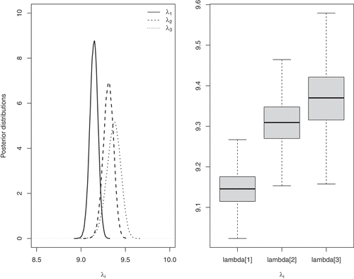
Table 3. Posterior summaries of ${\lambda }_i,i=1,2,3$

Parameter	Post. mean	Post. median	$95\mathrm{\%}$ HPD interval
${\lambda }_1$	$9.14$	$9.14$	$(9.05,9.23)$
${\lambda }_2$	$9.31$	$9.31$	$(9.19,9.42)$
${\lambda }_3$	$9.37$	$9.37$	$(9.21,9.52)$

3.1. Additional results

Mellinas et al. (2016) measured (positive) differences between Booking and Priceline systems, when testing for the existence of scoring differences between these systems (the null hypothesis), but with their frequentist procedure we can only accept or reject the null hypothesis based on its $p-$value, which, as we know, does not represent the chance that it is true (Assaf & Tsionas, 2018). The proposed Bayesian procedure provides a simple and intuitive solution to this concern, testing inequality hypotheses on the parameters as follows. Let us test the null hypothesis $H_0:{\lambda }_1>{\lambda }_2>\dots >{\lambda }_s$ vs $H_1:$ the ordering of the parameters is any other different permutation, with $1\le s\le k.$

Under the hierarchical model considered, we need to compute the posterior probability of the null space ${\mathrm{\Lambda }}_0=\left\{({\lambda }_1,\dots ,{\lambda }_s):{\lambda }_1>{\lambda }_2>\dots >{\lambda }_s\right\}$, which is found to be

(16) $Pr(H_0|n,t)={\int }_0^{\mathrm{\infty }}\left({\int }_{{\mathrm{\Lambda }}_0}\prod _{j=1}^s\mathrm{G}\mathrm{a}\mathrm{m}\mathrm{m}\mathrm{a}({\lambda }_j|t_j+\lambda ,n_j+1)d{\lambda }_j\right)\pi (\lambda |x)d\lambda ,$(16)

where $n=(n_1,\dots ,n_k)$ and $t=(t_1,\dots ,t_k).$ MCMC methods are useful here, as they take advantage of the posterior conditional independence of the ${\lambda }_j$ given $\lambda$, i.e., simulating first from the posterior of the hyperparameter $\lambda$, and then from Gamma distributions.

For instance, using the data of the motivating example, the (posterior) probability of ${\lambda }_1<{\lambda }_2$ is $0.98$. That is, there exists a probability of $0.98$ that the average score from the Booking population was lower than that from the TripAdvisor population. Similarly, the posterior probability of ${\lambda }_1<{\lambda }_3$ is $0.99$.

4. Drawing inferences on the overall score parameter $\lambda$: a BMA proposal

As shown in Table 2, there are five heterogeneity configurations, and choosing any one of these may overlook model selection uncertainty and misrepresent parameter uncertainty. To overcome this problem, we propose the use of Bayesian model averaging (BMA) techniques. Thus, instead of selecting one model and drawing inferences from it, we use weighted averages over the set of models to obtain the expectations and quantities of interest.

The BMA approach to drawing inferences on parameter $\lambda$ involves averaging over all models. For instance, the posterior distribution for the observed data is given by

(17) $\pi (\lambda |\mathrm{d}\mathrm{a}\mathrm{t}\mathrm{a})=\sum _{s=1}^{|{\mathcal{C}}_k|}\pi (\lambda |M_s,\mathrm{d}\mathrm{a}\mathrm{t}\mathrm{a})Pr(M_s|\mathrm{d}\mathrm{a}\mathrm{t}\mathrm{a}),$(17)

that is, the average of the posterior distributions under each of the models considered, weighted by its posterior model probability. The posterior probability for the model $M_s$ can be obtained by:

(18) $Pr(M_s|\mathrm{d}\mathrm{a}\mathrm{t}\mathrm{a})=\frac{Pr(M_s)Pr(\mathrm{d}\mathrm{a}\mathrm{t}\mathrm{a}|M_s)}{{\sum }_{s=1}^{|{\mathcal{C}}_k|}Pr(M_s)Pr(\mathrm{d}\mathrm{a}\mathrm{t}\mathrm{a}|M_s)},s=1,\dots ,|{\mathcal{C}}_k|,$(18)

where

(19) $Pr(\mathrm{d}\mathrm{a}\mathrm{t}\mathrm{a}|M_s)={\int }_{{\mathrm{\Lambda }}_s}Pr(\mathrm{d}\mathrm{a}\mathrm{t}\mathrm{a}|{\lambda }_s,M_s)Pr({\lambda }_s|M_s)d{\lambda }_s,$(19)

is the integrated likelihood of the model $M_s,$ ${\lambda }_s$ is the vector of parameters of model $M_s$, $Pr({\lambda }_s|M_s)$ is the prior density of ${\lambda }_s$ under model $M_s,$ $Pr(\mathrm{d}\mathrm{a}\mathrm{t}\mathrm{a}|{\lambda }_s,M_s)$ is the likelihood and $Pr(M_s)$ is the prior probability of model $M_s.$

Inference on the parameter $\lambda$ is also affected by the weights applied in expression (17). In particular, the posterior mean for $\lambda$ is the weighted average of the posterior means in each model:

(20) $\mathbb{E}(\lambda |\mathrm{d}\mathrm{a}\mathrm{t}\mathrm{a})=\sum _{s=1}^{|C_k|}\mathbb{E}(\lambda |M_s,\mathrm{d}\mathrm{a}\mathrm{t}\mathrm{a})Pr(M_s|\mathrm{d}\mathrm{a}\mathrm{t}\mathrm{a}).$(20)

4.1. Results (continued)

Returning to the dataset considered in the motivating example, from Table 2 we have different posterior probabilities for the cluster structures, and these probabilities are incorporated in the BMA of the overall average $\lambda$ score. All the measures of interest can be obtained from the BMA posterior distribution in (17). Table 4 shows the posterior summaries of the $\lambda$ score under each heterogeneity configuration, together with the proposed BMA.

Table 4. Posterior summaries of $\lambda$ under each model $M_i,i=1,\dots ,5$ and the proposed BMA

Model	Post. mean	Post. median	$95\mathrm{\%}$ Credibility interval
$M_1$	$8.60$	$8.75$	$(6.44,9.84)$
$M_2$	$8.71$	$8.78$	$(7.29,9.68)$
$M_3$	$8.72$	$8.80$	$(7.30,9.70)$
$M_4$	$8.76$	$8.84$	$(7.36,9.71)$
$M_5$	$8.78$	$8.83$	$(7.66,9.60)$
BMA	$8.69$	$8.78$	$(7.07,9.72)$

It is interesting to note the following. On the one hand, under the classical homogeneity partition, which assumes that all samples are obtained from the same population, the parameter of interest $\lambda$ would be underestimated (see Table 4 for the estimate corresponding to model $M_1$) and the uncertainty reflected by the credible interval is significantly larger. In contrast, the model with a greater likelihood, $M_2$, provides more accurate estimates with a significantly narrower credibility range than the prior model. Finally, the BMA model accumulates all the uncertainties associated with each of the potential models and combines them according to their probabilities of being true, as shown in Table 2.

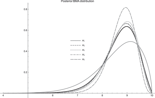
Figure 3 shows all the posterior distributions including the BMA posterior density of $\lambda$. It is apparent that the BMA posterior distribution of $\lambda$ represents a compromise between the posterior distributions under each heterogeneity model in which the weights from models $M_2$ and $M_1$ are greatest. As expected, this is reflected by a left—skewed posterior distribution, with a mode around $\lambda =9$.

Figure 3. Posterior distribution of $\lambda$ for each heterogeneity configuration (models $M_i,i=1,\dots ,5,$ in dashed grey lines) and the corresponding posterior BMA distribution (continuous black line).

5. Concluding remarks

In this paper, we employ a straightforward Bayesian approach to address the issue of comparing multiple populations of OCR scores. To determine the necessary Bayes factors for comparing each alternative with the baseline homogeneity model, we adopt a hierarchical model that assesses the homogeneity of the Poisson means. Bayesian practitioners base judgments on the posterior probability of all involved models, in contrast to the often inconclusive $p-$values used in frequentist approaches. This advantage allows Bayesian methods to quantify evidence supporting the null hypothesis of homogeneity and to simultaneously test multiple hypotheses—an area where frequentist methods fall short. The Bayesian approach bypasses these limitations, eliminating the need for ad—hoc thresholds, which can be essential in cases of small sample sizes ($k$), low parameter estimates (${\lambda }_i$), or varying sample sizes. The proposed Bayesian method is applicable in each of these scenarios.

Our paper presents a Bayesian clustering application involving three key online rating platforms. Extending this method to more platforms is feasible, though scalability might raise computational issues beyond 15 platforms due to the considerable number of clusters to be examined, as indicated by Bell’s number (Rota, 1964). Fortunately, Bign´e et al. (2020) recently reviewed numerous published studies analyzing eWOM ratings, with no more than 15 platforms included. Similar to Bign´e et al. (2020), which considered eight platforms, our paper offers implications for managers and analysts—emphasizing the importance of focusing on true overall average scores to optimize products and services, rather than excessive analysis of minor online rating fluctuations. Using a real—world case study to demonstrate the Bayesian model’s practicality reveals that our methods could deliver considerable results in online consumer reviews. This paper could be considered a further step towards this final objective.

Beyond the work by A. G. Assaf and Tsionas (2019), who applied Bayesian Model Averaging (BMA) to estimate dynamic panel data models in tourism research, few studies in this field have utilized the BMA procedure. We propose BMA as an intuitively appealing approach to addressing uncertainty in heterogeneity. This procedure facilitates inference generation about the true overall average $\lambda$ score by averaging heterogeneity models derived from clustering observed data.

Furthermore, our proposed Bayesian model offers a natural method to determine whether one sample population’s ratings surpass those of others. The clustering procedure described accounts for all heterogeneity structure uncertainties and identifies each feasible cluster model. This characteristic may also serve as a valuable starting point for exploring sources of heterogeneity before conducting simple model averaging, akin to Mellinas et al. (2016).

Acknowledgments

MME and FJVP were partially funded by grant PID2021–127989OB–I00 (Agencia Estatal de Investigación, Ministerio de Ciencia e Innovación, Spain).

Disclosure statement

No potential conflict of interest was reported by the author(s).

Additional information

Funding

This work was partially supported by the Agencia Estatal de Investigación (Ministerio de Ciencia e Innovación, Spain) under Grant PID2021–127989OB–I00.

Notes on contributors

M. Martel–Escobar

M. Martel–Escobar is a full Professor in mathematics for economics and business at the Faculty of Economics, Business and Tourism, University of Las Palmas de Gran Canaria (ULPGC), Canary Islands, Spain. Prof. Martel–Escobar is a research member of the Tourism and Sustainable Economic Development (TIDES) Research Institute at the ULPGC. Martel—Escobar’s research focused on applications of Bayesian methods to economics and business. Her recent publications appeared in leading applied statistics journals such as Journal of Applied Statistics, and Applied Stochastic Models in Business and Industry.

C. González-Martel

C. González–Martel, PhD in economics and business management, is an assistant Professor in mathematics for business at the Faculty of Economics, Business and Tourism, University of Las Palmas de Gran Canaria. His major research interests include data science in the contexts of tourism and hospitality. His recent publications appeared in leading tourism and hospitality journals such as Journal of Destination Marketing and Management, Tourism Management, and Tourism Economics.

F. J. Vázquez-Polo

F.J. Vázquez–Polo is a Chair Professor of Bayesian Methods at the University of Las Palmas de Gran Canaria (Canary Islands, Spain) and research member of the Tourism and Sustainable Economic Development (TIDES) Research Institute at the ULPGC. Prof. Vázquez–Polo is Head of the Department of Quantitative Methods at ULPGC. His research interests include Bayesian statistics as well as applications topics in economics, business and tourism, among others. His work has been published in statistics and economic journals such as Statistical Methods in Medical Research, European Journal of Operational Research, Communications in Statistics: Theory and Methods, and Journal of Business and Economic Statistics, among others.

Notes

1. The case study analysed in Bianchi and Heo (2021) presents a sample average score of 9.4 with a variance of 1.002 for score S, in contrast with a Poisson distribution sampling which the mean and the variance coincide. However, a simple linear transformation $10-S$, bringing the two measures into close proximity, produces a better fit to a Poisson distribution. In the present study, we adopt this procedure, thus obtaining a right—skewed (reverse J shaped) plot, as is usual for a Poisson distribution.

Appendix A

This appendix provides some technical details about the expressions considered in Section 2. Most of the results are derived from the well–known expression for the integral of the kernel of a Gamma density,

(A1) ${\int }_0^{\mathrm{\infty }}{z}^{\alpha -1}exp(-\beta z)dz=\frac{\mathrm{\Gamma }(\alpha )}{{\beta }^{\alpha }}.$(A1)

Now using (8), the likelihood function $f_1(c|\lambda )$ is obtained by integration

(A2) $\begin{array}{rl}& f_1(c|\lambda )={\int }_0^{\mathrm{\infty }}{f}_1(c_1,\dots ,c_s|{\lambda }_1,\dots ,{\lambda }_s)\pi ({\lambda }_1,\dots ,{\lambda }_s|\lambda )d{\lambda }_1\dots d{\lambda }_s\\ & =\prod _{j=1}^s\left({\int }_0^{\mathrm{\infty }}f(c_j|{\lambda }_j)\pi ({\lambda }_j|\lambda )d{\lambda }_j\right).\end{array}$(A2)

The integral in (A2) is obtained as

$\begin{array}{rl}& {\int }_0^{\mathrm{\infty }}f(c_j|{\lambda }_j)\pi ({\lambda }_j|\lambda )d{\lambda }_j={\int }_0^{\mathrm{\infty }}{\lambda }_j^{t_j}exp(-m_j{\lambda }_j)\frac{1}{\mathrm{\Gamma }(\lambda )}{\lambda }_j^{\lambda -1}exp(-{\lambda }_j)d{\lambda }_j\\ & =\frac{1}{\mathrm{\Gamma }(\lambda )}{\int }_0^{\mathrm{\infty }}{\lambda }_j^{t_j+\lambda -1}exp(-(m_j+1){\lambda }_j)d{\lambda }_j\\ & =\frac{1}{\mathrm{\Gamma }(\lambda )}\frac{\mathrm{\Gamma }(t_j+\lambda )}{{(m_j+1)}^{t_j+\lambda }},\end{array}$

Thus $f_1(c|\lambda )$ in (10) is given by

$f_1(c|\lambda )=\prod _{j=1}^s\left({\int }_0^{\mathrm{\infty }}f(c_j|{\lambda }_j)\pi ({\lambda }_j|\lambda )d{\lambda }_j\right)=\frac{1}{\mathrm{\Gamma }{(\lambda )}^s}\prod _{j=1}^s\frac{\mathrm{\Gamma }(t_j+\lambda )}{{(m_j+1)}^{t_j+\lambda }}.$

Appendix B

We must first compute the posterior distribution of the hyperparameter $\lambda$. Equation (12)(12) $\pi (\lambda )\propto {\lambda }^{-1/2}.$(12) provides the prior $\pi (\lambda )$, and using Equation (10)(10) $f_1(\mathbf{c}|\lambda )=\frac{1}{\mathrm{\Gamma }{(\lambda )}^s}\prod _{j=1}^s\frac{\mathrm{\Gamma }(t_j+\lambda )}{{(m_j+1)}^{t_j+\lambda }}.$(10) when computed for the homogeneity partition $x$, the integrated likelihood of the complete data is given by

(B1) $f(x|\lambda )\propto \frac{1}{\mathrm{\Gamma }{(\lambda )}^k}\prod _{i=1}^k\frac{\mathrm{\Gamma }(t_i+\lambda )}{{(n_i+1)}^{t_i+\lambda }}.$(B1)

Therefore, by Bayes theorem, the posterior density of $\lambda$ is proportional to

(B2) $\pi (\lambda |x)\propto \pi (\lambda )f(x|\lambda )={\lambda }^{-1/2}\frac{1}{\mathrm{\Gamma }{(\lambda )}^k}\prod _{i=1}^k\frac{\mathrm{\Gamma }(t_i+\lambda )}{{(n_i+1)}^{t_i+\lambda }}.$(B2)

from which the normalising constant is easily obtained by numerical integration. Now, given the hierarchical structure considered above, we can obtain the posterior distributions of the ${\lambda }_i$ in terms of the posterior of $\lambda$.

In fact, given $\lambda$ and $x$, it follows that ${\lambda }_i|\lambda ,x$ are conditionally independent and that each follows a Gamma distribution. Thus

(B3) $\pi ({\lambda }_i|\lambda ,\mathbf{x})=\mathrm{G}\mathrm{a}\mathrm{m}\mathrm{m}\mathrm{a}({\lambda }_i|t_i+\lambda ,n_i+1),$(B3)

and, consequently

(B4) $\pi ({\lambda }_i|x)={\int }_0^{\mathrm{\infty }}\mathrm{G}\mathrm{a}\mathrm{m}\mathrm{m}\mathrm{a}({\lambda }_i|t_i+\lambda ,n_i+1)\pi (\lambda |x)d\lambda .$(B4)

where $\mathrm{G}\mathrm{a}\mathrm{m}\mathrm{m}\mathrm{a}({\lambda }_i|t_i+\lambda ,n_i+1)$ denotes the Gamma distribution of the corresponding parameters.

Therefore, the posterior distribution for ${\lambda }_i$ ($i=1,\dots ,k$) can be computed either by numerical integration or by Markov chain Monte Carlo (MCMC) simulation. The MCMC implementation to find the posterior distributions is particularly easy to code and is preferred.

References

- Assaf, A. (2009). Are U.S. airlines really in crisis? Tourism Management, 30(6), 916–16. Retrieved from. https://doi.org/10.1016/j.tourman.2008.11.006
- Assaf, A. (2011). Accounting for technological differences in modelling the performance of airports: A Bayesian approach. Applied Economics, 43(18), 2267–2275. Retrieved from. https://doi.org/10.1080/00036840903101779
- Assaf, A. G. (2012). Benchmarking the Asia Pacific tourism industry: A Bayesian combination of DEA and stochastic frontier. Tourism Management, 33(5), 1122–1127. Retrieved from. https://doi.org/10.1016/j.tourman.2011.11.021
- Assaf, A. G., & Magnini, V. (2012). Accounting for customer satisfaction in measuring hotel efficiency: Evidence from the US hotel industry. International Journal of Hospitality Management, 31(3), 642–647. Retrieved from. https://doi.org/10.1016/j.ijhm.2011.08.008
- Assaf, A. G., & Tsionas, E. G. (2015). Incorporating destination quality into the measurement of tourism performance: A Bayesian approach. Tourism Management, 49, 58–71. Retrieved from. https://doi.org/10.1016/j.tourman.2015.02.003
- Assaf, A., & Tsionas, M. (2018). Bayes factors vs. p-values. Tourism Management, 67, 17–31. Retrieved from. https://doi.org/10.1016/j.tourman.2017.11.011
- Assaf, A., & Tsionas, M. (2019). Quantitative research in tourism and hospitality: An agenda for best–practice recommendations. International Journal of Contemporary Hospitality Management, 31(7), 2776–2787. Retrieved from. https://doi.org/10.1108/IJCHM-02-2019-0148
- Assaf, A. G., Tsionas, M., Kock, F., & Josiassen, A. (2021). A Bayesian non–parametric stochastic frontier model. Annals of Tourism Research, 87(103116), 103116. Retrieved from. https://doi.org/10.1016/j.annals.2020.103116
- Assaf, A. G., Tsionas, M., & Oh, H. (2018). The time has come: Toward Bayesian SEM estimation in tourism research. Tourism Management, 64, 98–109. Retrieved from. https://doi.org/10.1016/j.tourman.2017.07.018
- Barry, D., & Hartigan, J. A. (1992). Product partition models for change point problems. The Annals of Statistics, 20(1), 260–279. Retrieved from. https://doi.org/10.1214/aos/1176348521
- Bianchi, G., & Heo, C. (2021). A Bayesian statistics approach to hospitality research. Current Issues in Tourism, 24(22), 3141–3150. Retrieved from. https://doi.org/10.1080/13683500.2021.1896486
- Bign´e, E., William, E., & Soria-Olivas, E. (2020). Similarity and consistency in hotel online ratings across platforms. Journal of Travel Research, 59(4), 742–758. Retrieved from. https://doi.org/10.1177/0047287519859705
- Boto-Garc´ıa, D., Zapico, E., Escalonilla, M., & Baños Pino, J. F. (2021). Tourists’ preferences for hotel booking. International Journal of Hospitality Management, 92(102726), 102726. Retrieved from. https://doi.org/10.1016/j.ijhm.2020.102726
- Buhalis, D., & Law, R. (2008). Progress in information technology and tourism management: 20 years on and 10 years after the internet–the state of etourism research. Tourism Management, 29(4), 609–623. Retrieved from. https://doi.org/10.1016/j.tourman.2008.01.005
- Chen, K., Wang, P., & Zhang, H. (2021). A novel hotel recommendation method based on personalized preferences and implicit relationships. International Journal of Hospitality Management, 92, 102710. Retrieved from. https://doi.org/10.1016/j.ijhm.2020.102710
- Coenders, G., Ferrer-Rosell, B., & Mart´ınez-Garc´ıa, E. (2016). Trip characteristics and dimensions of internet use for transportation, accommodation, and activities undertaken at destination. Journal of Hospitality Marketing & Management, 25(4), 498–511. Retrieved from. https://doi.org/10.1080/19368623.2015.1034827
- Fang, B., Ye, Q., Kucukusta, D., & Law, R. (2016). Analysis of the perceived value of online tourism reviews: Influence of readability and reviewer characteristics. Tourism Management, 52, 498–506. Retrieved from. https://doi.org/10.1016/j.tourman.2015.07.018
- Farcomeni, A. (2008). A review of modern multiple hypothesis testing, with particular attention to the false discovery proportion. Statistical Methods in Medical Research, 17(4), 347–388. Retrieved from. https://doi.org/10.1177/0962280206079046
- Fong, L. H. N., Lam, L. W., & Law, R. (2017). How locus of control shapes intention to reuse mobile apps for making hotel reservations: Evidence from Chinese consumers. Tourism Management, 61, 331–342. Retrieved from. https://doi.org/10.1016/j.tourman.2017.03.002
- Hoffart, J. C., Olschewski, S., & Rieskamp, J. (2019). Reaching for the star ratings: A Bayesian–inspired account of how people use consumer ratings. Journal of Economic Psychology 72, 99–116. Retrieved from. https://doi.org/10.1016/j.joep.2019.02.008
- Lei, S. S. I., Nicolau, J. L., & Wang, D. (2019). The impact of distribution channels on budget hotel performance. International Journal of Hospitality Management, 81, 141–149. Retrieved from. https://doi.org/10.1016/j.ijhm.2019.03.005
- Mariani, M. M., & Borghi, M. (2018). Effects of the Booking.com rating system: Bringing hotel class into the picture. Tourism Management, 66, 47–52. Retrieved from. https://doi.org/10.1016/j.tourman.2017.11.006
- Mellinas, J. P., Mar´ıa-Dolores, S.-M.-M., & Bernal Garc´ıa, J. J. (2015). Booking.com: The unexpected scoring system. Tourism Management 49, 72–74. Retrieved from. https://doi.org/10.1016/j.tourman.2014.08.019
- Mellinas, J. P., Mar´ıa-Dolores, S.-M.-M., & Bernal Garc´ıa, J. J. (2016). Effects of the Booking.com scoring system. Tourism Management 57, 80–83. Retrieved from. https://doi.org/10.1016/j.tourman.2016.05.015
- Mellinas, J. P., & Martin-Fuentes, E. (2021). Effects of Booking.com’s new scoring system. Tourism Management, 85(104280), 104280. Retrieved from. https://doi.org/10.1016/j.tourman.2020.104280
- Nilashi, M., Ahani, A., Esfahani, M. D., Yadegaridehkordi, E., Samad, S., Ibrahim, O., Sharef, N.M., & Akbari, E. (2019). Preference learning for eco-friendly hotels recommendation: A multi-criteria collaborative filtering approach. Journal of Cleaner Production 215, 767–783. https://doi.org/10.1016/j.jclepro.2019.01.012
- Peng, H.-G., Zhang, H.-Y., & Wang, J.-Q. (2018). Cloud decision support model for selecting hotels on TripAdvisor.com with probabilistic linguistic information. International Journal of Hospitality Management, 68(1), 124–138. Retrieved from. https://doi.org/10.1016/j.ijhm.2017.10.001
- Plummer, M., Stukalov, A., & Denwood, M. (2016). Package Rjags. Retrieved November , 2022 cran.stat.unipd.it/web.packages/rjags/rjags.pdf
- Rota, G. (1964). The number of partitions of a set. American Mathematical Monthly, 71(5), 498–504. Retrieved from. https://doi.org/10.1080/00029890.1964.11992270
- S´anchez-Franco, M., Navarro-Garc´ıa, A., & Rond´an-Cataluña, F. (2019). A naive Bayes strategy for classifying customer satisfaction: A study based on online reviews of hospitality services. Journal of Business Reseach 101, 499–506. Retrieved from. https://doi.org/10.1016/j.jbusres.2018.12.051
- Scott, J. G., & Berger, J. (2006). An exploration of aspects of Bayesian multiple testing. Journal of Statistical Planning and Inference, 136(7), 2144–2162. Retrieved from. https://doi.org/10.1016/j.jspi.2005.08.031
- Xiang, Z., Du, Q., Ma, Y., & Fan, W. (2017). A comparative analysis of major online review platforms: Implications for social media analytics in hospitality and tourism. Tourism Management, 58, 51–65. Retrieved from. https://doi.org/10.1016/j.tourman.2016.10.001
- Zhao, Y., Xu, X., & Wang, M. (2019). Predicting overall customer satisfaction: Big data evidence from hotel online textual reviews. International Journal of Hospitality Management, 76(Part A), 111–121. Retrieved from. https://doi.org/10.1016/j.ijhm.2018.03.017