The role of climate smart agricultural practices on household income and food security: A propensity score matching approach

Abstract

The aim of this study was to assess the impacts of climate smart agricultural practices on household income and food security in Doyogena and Basona climate smart landscapes in Ethiopia. Data were collected from 796 randomly selected smallholder farmers from the two climate-smart villages of the Doyogena (399) and Basona (397) districts. Using a propensity score matching approach, this study examines the contribution of CSA practices to farm household income and food security. Our study finds that the adoption of CSA practices enhances household food security in Doyogena, whereas in Basona, the implementation of CSA practices improved the average annual income of households. This study suggests that the introduction of CSA practices and scaling up of these practices should be site-specific, but not a one-size-fits-all approach. Promoting and scaling up these practices may require assessing the needs and priorities of communities in different locations.

Keywords:

• climate smart agriculture
• propensity score matching
• food security
• household income
• Ethiopia

1. Introduction

This study is fostered by the EU-IFAD funded project with the goal of building rural livelihoods and improving resilience to climate change of smallholder farmers of East and West Africa among which Ethiopia was one of the target countries. The country is one of the most vulnerable to climate variability and climate change due to its high dependence on rain-fed agriculture and natural resources, and its relatively low adaptive capacity to deal with these expected changes (World Bank, 2020). Climate variability and food insecurity have always been features of Ethiopia (Lewis, 2017). There are many routes through which climate change can affect food security. One major route is through climate change affecting the amount of food, both from direct impacts on yields and indirect effects through climate change’s impacts on water availability and quality, pests, and diseases (FAO, 2015). Among the many development options that exist, climate smart agriculture (CSA) is a sustainable approach that can enhance agricultural productivity and income by adopting adaptation strategies, while promoting resilience to climate change and reducing greenhouse gas emissions (Engel & Muller, 2016; FAO, 2013b). The CSA approach is not a technique, or a new production system, but rather a three-tiered action-based approach to identify existing production systems that can address the interlinked challenges of food security and climate change (FAO, 2017). Technologies considered climate-smart, and the “smartness” of a given CSA technology are context-specific and can vary considerably between different production systems and locations (World Bank, 2019).

The CGIAR Research Program on Climate Change, Agriculture and Food Security (CCAFS) is partnering with farmers, development organizations, and national and international agricultural research organizations in East Africa to test and promote a portfolio of CSA technologies and practices with the aim of scaling up and giving out the appropriate options. The CCAFS started piloting the climate smart village (CSV) approach in East Africa in 2012. In each CSV, a portfolio of climate-smart interventions is introduced depending on the agro-ecological characteristics of the CSV, level of development, capacity, and interests of farmers and local government partners (Recha et al., 2017). In Ethiopia, the CCAFS has collaborated with local communities, government, and non-government organizations to establish two climate-smart landscapes: Doyogena in southern Ethiopia and Basona in central Ethiopia. Locally appropriate CSA practices are being tested and promoted at these sites. Despite the significant global action and investment being oriented towards CSA and the growing recognition of the potential of CSA in developing countries, relatively few studies have quantified the impact of these practices on farm household income and food security (CCAFS, 2016). Some stories of the success of CSA technologies and practices positively change the lives of farmers in Asia and Latin America. Monitoring and evaluation results from CSVs have shown that climate smart agriculture increases farmers’ productivity, income, and household food security in these regions (e.g., Hasan et al., 2018; Pal & Kapoor, 2020; WFO, 2020). Evidence from some East and Southern African countries also suggests that the introduction of CSA practices among farmers contributes to adaptation to a changing climate by improving agricultural income and food security (e.g., Mugabe, 2020; Mujeyi et al., 2021; Ogada et al., 2020; Siziba et al., 2019; Wekesa et al., 2018). However, the impact of these CSA practices on food security and income of Ethiopian farmers is not well documented and understood. The main objective of this study is to assess the impact of CSA practices on household income and food security in Doyogena and Basona CSVs. Estimation of the socio-economic impacts of these practices seeks to fill the knowledge gap and highlight the scaling up of appropriate CSA options. The specific objectives include: (i) estimating the impacts of CSA practices on household income and food security, (ii) documenting the role of CSA practices in enhancing the income and food security of farmers, and (iii) providing evidence that can help donors and decision makers justify funding and guide priorities in scaling up the adoption of CSA technologies and practices.

2. Methodology

2.1. Propensity score matching

Impact evaluation is essentially a problem of missing data (Ravallion, 2005). Determining the counterfactual is the pillar of sound impact evaluation (Heinrich et al., 2010). The standard setup in the treatment effect literature for basic impact evaluation that measures the direct effect of a program on outcomes can be stated as follows (Gertler et al., 2011):

(1) $Y_i=\alpha X_i+\beta T_i+{\epsilon }_{\hspace{0.17em}}$(1)

Where $Y_i$ denotes the outcomes (e.g., income or food security of household) $i$and $T_i$is a dummy variable equal to 1 for households who participate in the program (in this case, implementing CSA practices) and 0 otherwise. $X_i$is a set of observable household characteristics that influence household income and food security, and $\epsilon$ is an error term representing unobserved factors that affect household income and food security. The problem with estimating equation 1(1) $Y_i=\alpha X_i+\beta T_i+{\epsilon }_{\hspace{0.17em}}$(1) is that participating in the CSA program is not random because of reasons such as purposive program placement; that is, CSA programs can be implemented based on the needs of communities and self-selection into the program given program design and placement. Self-selection can be based on both observed and unobserved factors (Heckman & Navarro, 2004). In the case of unobserved factors, the error term $\epsilon$ in estimating Equation 1(1) $Y_i=\alpha X_i+\beta T_i+{\epsilon }_{\hspace{0.17em}}$(1) contains variables that are also correlated with the CSA program dummy $T$. In such a situation, one cannot measure and account for the unobserved factors in equation 1(1) $Y_i=\alpha X_i+\beta T_i+{\epsilon }_{\hspace{0.17em}}$(1) , which leads to an unobserved selection bias that violates one of the assumptions of ordinary least squares, that is, no correlation between explanatory variables and the error term (Berry, 1993). Randomized controlled trials are considered the gold standard approach for estimating the impact of a program on outcomes, because random treatment allocation ensures that treatment status will not be confounded with either measured or unmeasured characteristics (Greenland et al., 1999). However, randomly assigning a treatment or program raises concerns, including ethical issues, external validity, partial or lack of compliance, and spillovers (Khandker et al., 2010).

Propensity score matching (PSM) method is an alternative approach for estimating the impact of a program when random assignment of households into a program is not feasible (Rosenbaum & Rubin, 1983). The propensity score is defined as the probability of assignment to a particular treatment conditional on a vector of observed covariates (Rosenbaum & Rubin, 1983). There are two stages in the PSM method. In the first stage, using the entire sample and the binary outcome model, PSM estimates the probability of participating in the CSA program using the observed household characteristics $x$. This generates the propensity score$P\left(x\right)$, that is, the probability that a household with a vector of characteristic $x$ will participate in CSA practices. The vector $x$ represents observable variables that determine whether a household implements CSA. Households with similar observable characteristics are likely to have similar propensity scores$P\left(x\right)$. Based on the similarity in propensity scores, PSM constructs statistical comparison groups, that is, households with similar propensity scores $P\left(x\right)$, where one group has participated in CSA practices and the other group has not participated in CSA practices. Participants were then matched based on this probability or propensity score to non-participants, and unmatched units were dropped (Rubin, 2001). There are different matching techniques for implementing PSM. These include nearest neighbor matching, radius matching, kernel matching, and stratification or interval matching (Rosenbaum, 1999; Rubin, 2007).

In this study, we employe the Nearest Neighbor (NN) matching method and the Kernel matching method. In the NN matching method each treatment unit is matched to the comparison unit with the closest propensity score. This matching method is one of the most common and easiest to implement and understand. Since the NN matching method without restriction may lead to poor matches, we impose a caliper so that it can only select a match if it is within the caliper. In addition to the NN matching method, we employ the Kernel matching method. This method uses a weighted average of the outcome variable for all nonparticipants to construct the counterfactual outcome. By comparing results across these two matching algorithms, we show the robustness of the program effect.

After matching, a covariate balancing test was required to ensure that the differences in the covariates in the two groups of matched samples were removed for the matched groups to be credibly counterfactual (Ali & Abdulai, 2010). The second stage of PSM calculates the average outcome for participants and non-participants and then estimates the impacts of CSA practices as the difference in average outcomes between the two groups of households, which is called the average treatment effect on the treated (ATT). The ATT can be defined as follows:

(2) $ATT=E_{P\left(x\mathrm{\setminus }T=1\right)}[E\left\{Y_1\mathrm{\setminus }T=1,P\left(x\right)\right\}-E\left\{Y_0\mathrm{\setminus }T=0,P\left(x\right)\right\}]$(2)

Two assumptions underlie the PSM method. Unconfoundedness is the first assumption that the uptake of the program is based entirely on observed characteristics (Rosenbaum & Rubin, 1983). The second is the assumption of a common support or overlap condition. This condition ensures that the treatment observations have comparison observations near the propensity score distribution (Heckman et al., 1999).

2.2. Survey location and data collection

Household interviews were conducted in Ethiopia across two regions: the Amhara and Southern Nations, Nationalities, and People’s Region (SNNPR). Figure 1 1 shows the locations of the two surveys.

Figure 1. Map of Ethiopia and survey locations.

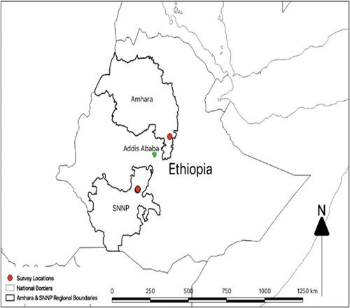
Doyogena District is located in the SNNPR of Ethiopia. The altitude ranges from 2420 to 2740 meters above sea level (m. a. s.l.). The mean annual rainfall ranges from 1,000 to 1,400 mm, while the temperature ranges from 12.6°C to 20°C. The farming system is characterized by an Enset (Ensete ventricosum)—cereal–livestock production system. The main crops grown include wheat, barley, legumes, and vegetables, such as potatoes. Enset, an important source of food, is grown in the area by almost all households. The average cropland size in the area was 0.6 hectare. Livestock production includes cattle, sheep, and poultry production. Subsistence farming in rain-fed areas is increasingly threatened by climate-related changes, such as greater variability in the expected onset and cessation of rain, heavy rain, strong winds, low temperatures, frost, and drought. Due to the steep slope topography, the area also suffers from land degradation and loss of soil fertility, which results in declining crop production and a lack of feed for livestock (Bonilla-Findji & Eitzinger, 2019). To address these challenges, locally relevant CSA practices that are both sustainable and resilient to climate change are being tested and promoted to improve farmers’ livelihoods. Approximately 11 CSA practices have been implemented in the Doyogena climate-smart landscape. These include soil and water conservation (SWC) practices such as soil bunds with Desho grass (Pennisetum pedicellatum); controlled grazing; improved wheat seeds (high yielding, disease resistant, and early maturing varieties), improved bean seeds (high yielding varieties), improved potato seeds (high yielding, larger tuber size varieties), cereal/potato-legume crop rotation (N fixing and non-N fixing); residue incorporation of wheat or barley; green manure: vetch and/or lupin during off-season (N fixing in time), improved breeds for small ruminants, agroforestry (woody perennials and crops), and cut and carry systems for animal feed.

The Basona District is located in the Amhara Regional State of Ethiopia. The altitude ranges from 1,300 to 3,650 m.a.s.l. Average temperature ranges between 6 and 20° °C, while the mean annual rainfall varies from 950 to 1200 mm. The main farming system is mixed crop-livestock farming. The major crops grown included barley and wheat. The average cropland size in the area was less than 1.4 hectare. The Basona landscape is subject to climate variability, soil erosion, and land degradation. Food insecurity and feed scarcity are the main challenges that adversely affect the livelihood of farmers in the area. In addition, crop diseases, especially faba bean, are a major concern (Tamene et al., 2017; Tigist, 2016) and to address the dual challenges of climate change and declining food security, the CCAFS has established CSVs in the district. Within each CSV, with the support of development partners, agricultural research institutes, and CGIAR centers, locally appropriate CSA practices and policies are being tested. The portfolio of CSA practices implemented in Bosana includes improved breeds (small ruminants and cattle), improved seed varieties, SWC such as soil bunds, soil bunds with biological measures such as phalaris and tree lucerne, trenches, enclosures, percolation pits, check-dams (gabion check-dams and wood check-dams), and gully rehabilitation.

The Rural Household Multi-Indicator Survey (RHoMIS) was employed to monitor the impact of CSA practices on household income and food security at the two sites. RHoMIS is a household survey tool designed to rapidly characterize the state and changes in farming households using a series of standardized indicators. It includes a modular survey tool, digital platform to store and aggregate incoming data, and analysis code to quantify indicators and visualize the results. For further details, the reader is referred to the RHoMIS website https://www.rhomis.org.

A simple random sampling technique was employed to select respondents from each district. Data were collected from 796 randomly selected smallholder farmers at two sites: 399 from Doyogena and 397 from Basona. Half of the sample farmers were from the group implementing CSA practices (beneficiary group), whereas the remaining half were from farmers who did not implement CSA practices (control group). Prior to data collection, enumerator training was conducted on the use of the RHoMIS tool and a questionnaire that ran on ODK software to ensure that they were confident in using the software and the digital interface of data collection. In addition to the training, a field practice was organized to test the survey tool in the field with real farmers, where nine household heads from each district participated. The data were collected from 24 December 2020, to 5 January 2021, in Doyogena, and from 4 February to 16, 2021, in Basona district. The main topics covered in the survey included farm household demographic characteristics, farm size, land management, provision of climate information services (CIS) and extension services, SWC practices, crop and livestock production, farm and off-farm income, and household food security. The household food security indicators generated from the data were the household dietary diversity score (HDDS) and Food Insecurity Experience Scale (FEIS). The HDDS is meant to reflect, in a snapshot form, the economic ability of a household to access a variety of foods (FAO, 2013a; Swindale & Bilinsky, 2006) An increase in dietary diversity score is associated with socio-economic status and household food security. In this survey, the HDDS was calculated by asking respondents the frequency with which they consumed 10 different food groups within the last month. The typical FIES survey module contains eight questions focused on food-related behaviors and experiences associated with difficulties in accessing food due to resource constraints in the last 12 months (Ville et al., 2019). These experiences were linked to different severities of food insecurity in the survey: severe, moderate, mild, and food security. A higher number (numbers ranging from 0 to 8) indicates a greater experience of hunger (Radimer et al., 1990, 1992; Smith et al., 2017).

3. Results

3.1. General household characteristics

The summary of variables used in the empirical analysis, together with the X² and t-test results of the two districts (Doyogena and Basona), are presented in Table 1. A distinction was made between beneficiary households implementing CSA and control households (not implementing CSA).

Table 1. Descriptive statistics of sample respondents in the two districts

Variables	Doyogena		Basona		Doyogena t-test/X^2	Basona t-test/X^2
	Control	Beneficiary	Control	Beneficiary
Household characteristics
Average age (years)	45	45	45	47	0.64	0.26
Share male (%)	80	87	89	86	0.08	0.38
Education level (%)					0.00***	0.03***
No schooling	35	23	42	27
Adult education	0.5	0.5	17	20
Primary school	42	62	35	41
Secondary school	18	12	6	10
College	5	2	0.5	0.9
Household size (persons)	6	7	4	4	0.00***	0.00***
Household size in MAE	4.9	5.8	4	3	0.00***	0.00***
Land holding (ha)	0.6	0.6	1.4	1.4	0.47	0.82
Cultivated land (ha)	0.6	0.5	1.2	1.2	0.29	0.38
Total income (US$/year)	1163	1945	1365	3348	0.02***	0.00***
Livestock holding (TLU)	2.5	2.7	4.5	4.8	0.18	0.62
CSA practices
SWC (%)	41	96	98	99	0.00***	0.55
Agroforestry (%)	21	32	1.1	4.3	0.02***	0.05
Improved breed (%)	46	62	28	49	0.00***	0.00***
Improved seed (%)	6	20	12	15	0.00***	0.43
Agro advisory services
Extension services (%)	16	60	35	37	0.00***	0.62
CIS (%)	44	58	45	64	0.00***	0.00***
Household food security
FIES (Median)	7	5	2	2	0.00***	0.08
HDDS (Median)
Lean season	3	2	3	4	0.00***	0.07
Flush season	5	4	4	4	0.21	0.00***

Note: *, **, and *** mean values are significantly different at the 10%, 5%, and 1% levels respectively.

3.1.1. Doyogena

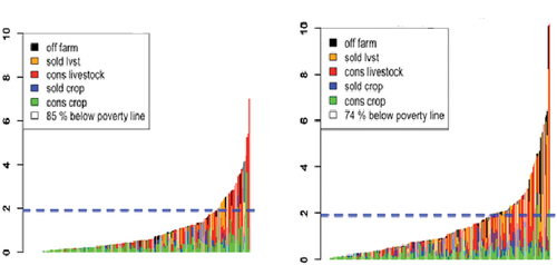
The majority of the respondents in both the beneficiary and control groups were men, with an average age of 45 years and mean family size of 7 and 6 for the beneficiary and control groups, respectively. Household size in the male adult equivalent (MAE) was 5.8 in the beneficiary group and 4.9 in the control group, respectively. More than one-third of the respondents from the control group were illiterate, while the majority of respondents from the beneficiary group were literate. The average land holding in both groups was 0.6 hectare and the average cultivated land in the control group was 0.6 and in the beneficiary group it was 0.5. The average livestock holding was 2.7 and 2.5 TLU¹ in the beneficiary and control groups, respectively. The average total income in the last 12 months was US$ 1164 in the control and US$ 1945 in the beneficiary group. The total values of household income and agricultural production for the control and beneficiary groups are shown in Figure 2. The height of each bar represents the total value of the USD per household member per day. The colors within the bars show where income or value came from crops, crops, and livestock sold and paid off-farm activities. Note that, owing to the differing number of interviews in each CSV, there are differing numbers of vertical bars, as each bar represents one household. Beneficiary households are better off than the control households. Although both groups displayed similar patterns in terms of value-added sources, beneficiary households reported greater value derived from selling livestock. Almost all beneficiaries and 41% of the control group were involved in SWC. Nearly one-third of beneficiaries and one-fifth of the control group practiced agroforestry. According to the sample respondents, CIS was communicated to 58% of beneficiaries and 44% of the control group. Similarly, 60% of beneficiaries and 16% of control farmers received advice from extension agents. One-fifth of the beneficiaries adopted improved seeds when only a few used it in the control group. The use of improved breeds was more widespread among the beneficiaries than in the control group, where less than half of them adopted it. Households in the beneficiary group reported medium food insecurity, scoring 5 out of a possible 8, while the control group experienced severe food insecurity, scoring 7 out of 8. The HDDS shows that control households performed better than beneficiary households in both flush and lean seasons. The control households scored 3 out of 10 and 5 out of 10 in the lean and flush seasons, respectively. Beneficiary households scored 2 out of 10 and 4 out of 10 in the lean and flush seasons, respectively.² The X² test demonstrates strong evidence of a significant relationship between most farm household characteristics and whether the household is in the control or beneficiary group. The t-test showed that there were significant differences in household size, household size MAE, income, FIES, and HDDS-LS between the control and beneficiary groups.

Figure 2. Total values of activities in Doyogena district – control and beneficiary groups from left to right.

3.1.2. Basona

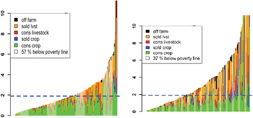
Most respondents in both the beneficiary and control groups were male, with an average age ranging between 45 and 47 years and a mean family size of 4. The household sizes in the male adult equivalent were four and three in the control and beneficiary groups, respectively. More respondents in the control group were illiterate than those in the beneficiary group. Similarly, the proportion of respondents who participated in adult education was higher in the beneficiary group than that in the control group. In both groups, less than half of the respondents had completed primary and secondary schools. The average landholding in both groups was 1.4 hectare while the average cultivated land for both groups was 1.2 hectare. The average livestock holding was 4.5 and 4.8 TLU in the control and beneficiary groups respectively. The average total income in the last 12 months was reported to be US$ 1366 and US$ 3349 in the control and beneficiary groups, respectively. Figure 3 shows the total household income and agricultural production for both groups. The height of each bar represents the total value in terms of USD per household member per day, while the colors within the bars show the sources of income or value, that is, crops consumed, crops sold, livestock sold, and paid off-farm activities. Each bar represents one household, and the differing number of vertical bars shows the differing number of interviews for each CSV. Beneficiary households were wealthier than those in the control group were. The main drivers appear to be the value of livestock sold (orange) and the crops consumed (green). The control group presented a similar pattern to beneficiary households but without the value gained from livestock sales. Almost all beneficiaries and control farmers were involved in SWC practices, whereas agroforestry was rarely reported in either group. CIS was communicated to 64% of the beneficiaries and 45% of the control group, while extension services were delivered to only 37% of the beneficiaries and 35% of the control group. Less than one-fifth of the respondents in both groups adopted improved seeds. There were more adopters of the improved breed in the beneficiaries than in the control group. Both beneficiary and control households scored mild food insecurity (2 out of 8). Regarding HDDS, both beneficiary and control households scored similar HDDS (4 out of 10) in the flush season, but in the lean season, beneficiary households scored more (4 out of 10), and the control group scored less (3 out of 10). According to the t-test, household size, household size, MAE, income, and HDDS-FS were significantly different between the control and beneficiary groups. When we look at the X² test, there is strong evidence of an association or correlation between the level of education, receiving CIS, use of improved breeds, and whether the household is in the control or beneficiary group.

Figure 3. Total values of activities in Basona district – control and beneficiary groups from left to right.

In summary, the descriptive analysis showed a difference between the two districts in terms of household characteristics, farm income and productivity, adoption of CSA practices, and household food security. In Basona, the average household size measured using MAE was smaller than that of Doyogena. Beneficiary households in Basona tend to be similar in size to control households, whereas in Doyogena, beneficiary households tend to be 1MAE larger than control households. Cultivated land was almost twice as large as that of Doyogena. In both districts, beneficiary farms tend to be very similar in size to the control farms. Livestock holdings were almost 2 TLUs larger in Basona than in Doyogena. In Basona, beneficiary households were wealthier than the control households and both household groups in Doyogena. Similarly, the second wealthiest group was the control households in Basona, which presented a similar pattern to beneficiary households but without the value gained from livestock sales. Comparing beneficiary and control households in Doyogena, the former was wealthier than the latter; however, both household groups were less wealthy than both household groups in Basona.

Almost all respondents in Basona and beneficiary households in Doyogena have implemented soil and water conservation practices. There was better adoption of improved breeds in both groups in Doyogena than in Basona. With improved seed adoption, Basona performed better than Doyogena. Regarding the FIES, both household groups in Basona reported mild food insecurity, whereas beneficiary and control households in Doyogena experienced medium and high food insecurity, respectively. In contrast, the HDDS suggested that there was a nutritionally inadequate and relatively scarce diet across the survey population.

3.2. Econometric model results

The impact of CSA on household income and food security was estimated using propensity score matching. The food security indicator selected for this analysis was the Food Insecurity Experience Scale (FIES) instead of the household dietary diversity score (HDDS). The main reason is that the FIES is a new approach introduced very recently, and it is the only food insecurity measure that provides the opportunity to generate internationally comparable, standard measures of food insecurity with details on levels of severity (Ville et al., 2019). In this analysis, the matching procedure was conducted using psmatch2 command in STATA, version 15. The analysis employed kernel and nearest-neighbor matching algorithms and imposed a common support condition to ensure proper matching. The average treatment effect on the treated (ATT) was compared between the two algorithms. The probit model estimation results for Doyogena and Basona are presented in Tables 2–3. The predicted outcome of the probit model represents the estimated probability of participation, that is, the propensity score; hence, this study does not focus on the relationship between the covariates and the dependent variable (probability of participation).

Table 2. Probit model for adoption of improved breed and SWC in Doyogena

Independent variables	Improved breed VS income		Improved breed VS FIES		SWC VS income		SWC VS FIES
	Coefficients	SE	Coefficients	SE	Coefficients	SE	Coefficients	SE
Age	0.00	0.00	0.00	0.00	0.00	0.01
Education	0.24***	0.06	0.21***	0.06
Gender	0.01	0.18	0.05	0.18	0.16	0.19
Land holding							0.11**	0.05
Cultivated land	0.02	0.05			−0.06	0.08
Household size	0.03	0.03			0.06**	0.03
Household size in MAE			0.02	0.04			0.07*	0.04
TLU							−0.02	0.04
Total income			0.00***	0.00			0.00**	0.00
Agroforestry			0.21	0.15
Extension service	0.44***	0.14			1.30***	0.17	1.34***	0.18
CIS	−0.07	0.13					−0.03	1.15
Constant	−0.66**	0.36	−0.53	0.35	−0.37	0.37	−0.34	0.24
No. of observation	399
LR X^2 (7)	32.26
LR X^2 (6)			31.26
LR X^2 (5)					78.74
LR X^2 (6)							89.10
Prob > X^2	0.00		0.00		0.00		0.00
Pseudo R^2	0.06		0.06		0.16		0.18

Note: *, **, and *** mean values are significantly different at the 10%, 5%, and 1% levels respectively.

Table 3. Probit model for adoption of improved breed and seed in Basona

Independent variables	Improved breed VS income		Improved breed VS FIES		Improved seed VS income		Improved seed VS FIES
	Coefficients	SE	Coefficients	SE	Coefficients	SE	Coefficients	SE
Age	0.00	0.00	0.00	0.00	0.01	0.01	0.01	0.01
Education	−0.00	0.06	0.01	0.06	0.16**	0.08	0.15*	0.08
Gender	0.42**	0.22			0.04	0.24	0.01	0.25
Land holding			0.02	0.03
Cultivated land	0.11	0.08			−0.25*	0.15	−0.29**	0.15
Household size	0.04	0.04	0.07*	0.04	−0.01	0.05
Household size in MAE							−0.00	0.06
TLU	0.01	0.01
Total income							0.00**	0.00
Agroforestry							0.10	0.47
Extension service	0.12	0.14			−0.16	0.17	−0.11	0.17
CIS					0.05	0.16
Constant	−1.19***	0.37	−0.82***	0.34	−1.32***	0.46	−1.38***	0.46
No. of observation	396
LR X^2 (7)	13.75
LR X^2 (4)			4.86
LR X^2 (7)					10.00
LR X^2 (8)							14.32
Prob > X^2	0.05		0.30		0.19		0.07
Pseudo R^2	0.03		0.01		0.03		0.04

Note: *, **, and *** mean values are significantly different at the 10%, 5%, and 1% levels respectively.

The results of the average treatment effect on the treated (ATT) are compared between the two matching algorithms (Tables 4 and 5). In Doyogena, improved breed and SWC practices were the two CSA practices used to examine their impact on outcome variables. The estimation results indicate that beneficiary households who adopted the improved breed gained significant average annual income that ranges between US$ 517 (ETB 21,197) and US$ 537 (ETB 22,017) compared to the control group who did not adopt the improved breed. In addition, there is a significant inverse relationship between the adoption of improved breeds and the scale of household food insecurity experience. This implies that beneficiary households that adopted an improved breed managed to reduce their food insecurity experience (experience of hunger) by a scale of 1.2 to 1.4 compared to the control households. The adoption of soil and water conservation practices had a similar significant positive impact on the income of beneficiary households. Accordingly, the implementation of soil and water conservation practices improved the average annual income of adopters to between US$ 349 (ETB 14,309) and US$ 504 (ETB 20,664). Comparing the food insecurity experience scale of those who implemented soil and water conservation and those who did not, the former group showed a significant reduction in food insecurity experience (experience of hunger) by a scale of 1.7 for both matching algorithms.

Table 4. Average treatment effect (ATT) of improved breed and SWC and sensitivity analysis in Doyogena

Matching algorithm	Livelihood outcome	ATT	T-statistics	Critical value ($\mathrm{\Gamma }$)	Beneficiary (n)	Control (n)
Average treatment effect of improved breed
Kernel	Income (US$/yr.)	517	2.95***	1.1–1.2	213	183
	FIES	−1.2	−4.12***	1.9–2.0	202	183
Nearest neighbor	Income (US$/yr.)	537	2.78***	1.1–1.2	213	183
	FIES	−1.4	−3.82***	1.8–1.9	202	183
Average treatment effect of SWC
Kernel	Income (US$/yr.)	349	2.14**	1.1–1.2	235	124
	FIES	−1.7	−3.88***	2.4–2.5	237	124
Nearest neighbor	Income (US$/yr.)	504	3.02***	1.1–1.2	236	124
	FIES	−1.7	−2.9***	2.3–2.4	237	124

Note: *, **, and *** mean values are significantly different at the 10%, 5%, and 1% levels respectively.

Table 5. Average treatment effect (ATT) of improved breed and seed and sensitivity analysis in Basona

Matching algorithm	Livelihood outcome	ATT	T-statistics	Critical value ($\mathrm{\Gamma }$)	Beneficiary (n)	Control (n)
Average treatment effect of improved breed
Kernel	Income (US$/yr.)	1825	4.3***	1.7–1.8	151	242
	FIES	−0.3	−1.73	1.4–1.5	154	242
Nearest neighbor	Income (US$/yr.)	1610	3.71***	1.6–1.7	154	242
	FIES	−0.7	−2.72***	1.4–1.5	154	242
Average treatment effect of improved seed
Kernel	Income (US$/yr.)	1245	1.83*	1.1–1.2	55	341
	FIES	−0.1	−0.35	-	54	341
Nearest neighbor	Income (US$/yr.)	1380	1.84*	1.1–1.2	55	341
	FIES	−0.7	−1.79*	-	55	341

Note: *, **, and *** mean values are significantly different at the 10%, 5%, and 1% levels respectively.

In Basona, improved breed and improved seed are the two climate smart agricultural practices used to examine their impacts on household income and food security. The adoption of improved breeds among beneficiary farmers significantly increased the average annual income between US$ 1610 (ETB 66,010) and US$1825 (ETB 74,825). Similarly, beneficiaries who adopted the improved seed variety gained a significant amount of average annual income that ranged between US$ 1245 (ETB 51,045) and US$ 1380 (56,580) compared to the control group. Looking at food security status, the adoption of improved breed among beneficiary farmers reduced the food insecurity experience by a scale of 0.3 to 0.7 compared to the control households. However, there was no significant relationship between adoption of improved seed and food security status.

3.3. Sensitivity analysis

Matching aims to achieve a balance on observed covariates, but there is no guarantee that matching will result in a balance between unobserved covariates and entirely reduce hidden bias. Sensitivity analysis appraises how the conclusions of a study might be altered by hidden biases of various magnitudes (Rosenbaum, 2010). According to Diprete and Gangl (2004), if the value of gamma in sensitivity analysis is the lowest and encompasses zero, then the probability of unobserved characteristics is relatively high, and the estimated impact is sensitive to the existence of unobservable characteristics. To analyze the degree to which selection of the unobservable may bias our inferences about the impacts of CSA practices on household income and food security, this study employed Rosenbaum’s (2002) procedure. Tables 4 and 5 present the sensitivity analysis results for the two districts. The results of the Rosenbaum sensitivity analysis test show that in Doyogena district, the critical level of $\mathrm{\Gamma }$, at which we would have to doubt the results of the positive impacts of improved breed and SWC practices on total income is between 1.1 and 1.2, which is highly sensitive to the presence of possible hidden bias due to unobserved confounders. Whereas the critical level of $\mathrm{\Gamma }$at which we would have to question the estimated results of the positive impacts of improved breed and SWC on food security are between 1.9–2.0 and 2.4–2.5, respectively. This means that our results are less sensitive to conclusions influenced by hidden biases.

In Basona District, for the estimation result of the impact of improved breed on total income to be sensitive to unobserved confounders, the critical level of $\mathrm{\Gamma }$must attain values between 1.7 and 1.8, which indicates the robustness of the result to hidden bias. Unlike the above result, the impact of improved seed on total income is the least robust to the possible presence of selection bias, with a critical $\mathrm{\Gamma }$value of 1.1 1.2. The sensitivity test for the impact of improved breed on food security shows the critical level of $\mathrm{\Gamma }$ at which we would have to defend our conclusion that the positive impact of improved breed on food security is between 1.4 and 1.5 (kernel matching) and between 1.5 and 1.6 (nearest neighbor matching).

3.4. Balancing test

The covariate balancing test was conducted using the pstest command in STATA 15. The pstest calculates several measures of balancing covariates before and after matching for the two districts in Tables 6 and 7. From the results of the balancing test, it is clear that after the variables are matched, they are balanced between the treatment and control groups. For each outcome variable in each district, the sample differences in the unmatched case surpassed the samples of the matched cases, indicating that the matching process resulted in significant bias reduction and a higher degree of covariate balance between the control and treatment samples used in the estimation procedure. Similarly, the insignificant t-test and the percentage bias reduction, which is less than 5% after matching in almost all cases, is an indication of achieving balance through the matching process. Other important balancing indicators that confirmed the covariate balancing across the two groups included the low pseudo R², the insignificant p-value of the likelihood ratio, and the low mean and median bias, which was below 5%.

Table 6. Matching quality test for Doyogena

Matching algorithm		Pseudo R^2	LR X^2	P> X^2	Mean Bias	Median Bias
Impact of improved breed on income
Kernel	U	0.05	32.26	0.00	18.7	16.5
	M	0.00	0.82	0.99	2.8	8.8
Nearest neighbor	U	0.05	32.26	0.00	18.7	16.5
	M	0.00	1.60	0.98	3.2	2.1
Impact of improved breed on FIES
Kernel	U	0.05	31.26	0.00	23.2	19.0
	M	0.00	0.88	0.99	2.9	1.9
Nearest neighbor	U	0.05	31.26	0.00	23.2	19.0
	M	0.01	5.91	0.43	5.8	3.2
Impact of SWC on income
Kernel	U	0.15	78.74	0.00	34.5	20.8
	M	0.01	8.25	0.14	6.9	3.0
Nearest neighbor	U	0.15	78.74	0.00	34.5	20.8
	M	0.00	3.16	0.67	3.5	3.1
Impact of SWC on FIES
Kernel	U	0.17	86.19	0.00	38.7	23.7
	M	0.00	1.72	0.88	4.5	4.0
Nearest neighbor	U	0.17	86.19	0.00	38.7	23.7
	M	0.00	1.72	0.88	2.6	2.4

Note: U= Unmatched; M=Matched.

Table 7. Matching quality test for Basona

Matching algorithm		Pseudo R^2	LR X^2	P> X^2	Mean Bias	Median Bias
Impact of improved breed on income
Kernel	U	0.02	13.75	0.05	15.0	19.3
	M	0.03	15.11	0.03	4.6	2.5
Nearest neighbor	U	0.02	13.75	0.05	15.0	19.3
	M	0.00	2.38	0.94	4.4	4.1
Impact of improved breed on FIES
Kernel	U	0.01	4.86	0.30	10.7	9.7
	M	0.00	0.63	0.96	4.1	3.9
Nearest neighbor	U	0.01	4.86	0.30	10.7	9.7
	M	0.00	1.56	0.82	5.2	4.4
Impact of improved seed on income
Kernel	U	0.03	10.01	0.18	14.8	13.9
	M	0.00	0.25	1,00	3.1	9.4
Nearest neighbor	U	0.03	10.01	0.18	14.8	13.9
	M	0.01	1.80	0.97	4.7	1.6
Impact of improved seed on FIES
Kernel	U	0.04	14.32	0.07	16.0	13.6
	M	0.00	0.99	0.99	4.1	2.6
Nearest neighbor	U	0.04	14.32	0.07	16.0	13.6
	M	0.01	2.81	0.90	11.5	11.1

Note: U= Unmatched; M=Matched.

4. Discussion

This study examines the impact of climate smart agricultural practices on household income and food security status in two districts of Ethiopia. Data were collected from 796 randomly selected smallholder farmers from the two districts, where 399 were selected from Doyogena and 397 from Basona. Half of the sample farmers were from the group that implemented climate smart agricultural practices (beneficiary group), whereas the remaining half were from farmers who did not implement climate smart agricultural practices (control group). Using a propensity score matching approach, this study examines the contribution of climate smart agricultural practices to farm household food security and income. The PSM method is a widely used approach when there are no baseline data, and hence, the reason for adopting this approach in our study.

The econometric model results show that in the Doyogena district, beneficiaries who adopted improved breed and soil and water conservation practices significantly increased their average annual income, where the significance of the increase was associated with a t-value of 2.95 and 2.78 for kernel and nearest neighbor matching algorithms, respectively. However, sensitivity analysis shows that these conclusions are prone to hidden bias due to unobserved confounders. Nonetheless, it is very important to recognize that while the sensitivity analysis provides information about the level of uncertainty contained in matching estimators by indicating the influence of a confounding variable, one cannot completely rule out the presence of a true positive impact of the use of improved breeds and soil and water conservation on household income in this study. This is because the sensitivity analysis results are worst-case scenarios or the most extreme situations that can occur (Diprete & Gangl, 2004). When we look at the impacts of these CSA practices on household food security, there was a significant improvement in household food security status, that is, a reduction in the food insecurity experience scale, which can also be described as a reduction in the experience of hunger. This result is illustrated by a significant t-value of − 4.12 and − 3.82 for kernel and nearest neighbor matching algorithms, respectively. The plausibility of this result was confirmed by a sensitivity test result that was highly robust to the possible presence of selection bias. This finding is in line with Mujeyi et al. (2021), Ogada et al. (2020), and Fentie and Beyene (2018), who assessed the impact of climate smart agricultural practices on household livelihood outcomes in Zimbabwe, Kenya, and Ethiopia.

Turning to the Basona District, the results indicate that the adoption of improved breed and seed beneficiary households achieved a significant amount of average annual income gain. The t-statistics supported the significance of the results with t-value of 4.3 and 3.7 for the improved breed and seed for kernel and nearest neighbor matching algorithms, respectively. The sensitivity test was also in agreement with these results, demonstrating the robustness of the results. Our findings are consistent with those of Mujeyi et al. (2021), who investigated the positive impact of climate smart agricultural technologies on household food security and income in smallholder integrated crop-livestock farming systems in Zimbabwe. Similarly, Wordofa et al. (2021) reported that in eastern Ethiopia, beneficiary households that adopted improved crop and livestock technologies gained higher annual income compared to the control group. Regarding food security status, our results indicated that household food security status has improved for those who maintain an improved breed. That is, there was a significant reduction in the experience of hunger among beneficiaries who adopted an improved breed, which was demonstrated in T-statistics of − 1.73 and − 2.72 for kernel and nearest neighbor matching algorithms, respectively. The sensitivity test revealed some degree of robustness of the estimation results to hidden bias. Similar studies, such as Wekesa et al. (2018) and Kifle (2020), who studied the impact of climate-smart agricultural practices on household food security in Kenya and Ethiopia, have reported the potential of CSA practices to alleviate food insecurity among smallholder farmers. Our results demonstrate that the implementation of climate smart agricultural practices contributed differently to the two districts. In Doyogena, CSA practices were important in reducing the incidence of hunger and improving the food security status of households, whereas in Basona district, CSA practices increased households’ annual income. These results are in line with our descriptive analysis, where beneficiaries in Doyogena reported a higher food insecurity experience scale compared to beneficiaries in Basona, where food insecurity was not much of a concern.

5. Conclusion and policy implication

The introduction of CSA practices and the scaling up of these practices should not be a one-size-fits-all approach. Promoting and scaling up these practices may require assessing the needs and priorities of communities in different locations. In food insecure communities, the type of CSA practice that has to be introduced may need to consider those practices that contribute more towards the enhancement of household food security. On the other hand, in food-secure communities, the kind of practices that must be promoted may need to be related to income-generating CSA practices. Identifying the appropriate CSA option for a specific location can help decision-makers and funding agencies guide priorities in scaling up the adoption of CSA practices.

Finally, one caveat of our study is the lack of baseline data, which resulted in the use of cross-sectional data and the PSM approach. This may have influenced the estimation results owing to the limitations associated with the use of the PSM approach. In impact analysis, a powerful measure of the impact of a treatment is using panel data collected from a baseline survey administered to both participants and nonparticipants before the program was implemented and after the program had been operating for some time. The estimation of impact analysis using panel data alleviates unobserved variable bias (Khandker et al., 2010). Nonetheless, our study is an important first step in providing useful baseline information for the upcoming monitoring and evaluation of CSA practices in the two districts.

Author(s) contribution statement

Abonesh Tesfaye: Conceptualization, methodology, data collection, analysis, and drafting of the manuscript.

James Hammond: Introducing and training on the Rural Household Multi-Indicator Survey (RHoMIS) tool and reviewing and editing the manuscript.

Maren Radeny: Reviewing and editing of the manuscript.

John Walker Recha: Supervision, reviewing and editing of the manuscript.

Abebe Nigussie: Data collection, reviewing and editing of the manuscript.

Gebermedihin Ambaw: Data collection, reviewing and editing of the manuscript.

Mark T. van Wijk: Introducing and training on the Rural Household Multi-Indicator Survey (RHoMIS) tool and reviewing and editing the manuscript.

Lulseged Tamene: Reviewing and editing of the manuscript.

Wuletawu Abera: Reviewing and editing of the manuscript.

Getamesay Demeke: Reviewing and editing of the manuscript.

Dawit Solomon: Supervision, reviewing and editing of the manuscript.

Acknowledgments

The authors are grateful to the European Commission and International Fund for Agriculture Development (EC-IFAD) Building Livelihood and Resilience to Climate Change in the East and West Africa Project (G158), which financed the assessment of the impacts of climate smart agriculture on household income and food security in the Doyogena and Basona climate smart villages. This study was also partially funded by the Accelerating Impacts of CGIAR Climate Research for Africa (AICCRA) project supported by a grant from the International Development Association (IDA) of the World Bank, which helps deliver a climate-smart African future driven by science and innovation in agriculture for Africa.

Disclosure statement

No potential conflict of interest was reported by the authors.

Additional information

Funding

This work was supported by the European Commission and International Fund for Agriculture Development (grant number EC-IFAD, CIA017) and the International Development Association (IDA) of the World Bank through the AICCRA project (grant number AICCRA, CIA020).

Notes on contributors

Abonesh Tesfaye

Abonesh Tesfaye holds a Ph.D. in Environmental Economics from Vrije Universiteit in Amsterdam. She is a Senior Research Consultant at AICCRA Ethiopia and East and Southern Africa programme at ILRI, Ethiopia.

John Walker Recha

John W. Recha holds a Ph.D. in Soil and Crop Sciences at Cornell University. He is a Climate-Smart Agriculture and Policy Scientist at AICCRA East and Southern Africa programme at ILRI, Kenya.

Lulseged Tamene

Lulseged Tamene Desta holds a Ph.D. in Landscape Ecology from the Center for Development Research, Germany. He is Director, Multifunctional Landscape at the Alliance of Bioversity & CIAT, Ethiopia.

Getamesay Demeke

Getamesay Demeke is a project coordinator at Inter Aide, Ethiopia. He has an agriculture and project management background.

Dawit Solomon

Dawit Solomon holds a Ph.D. in Geoecology and Soil Science from the University of Bayreuth. He is the Regional Program Leader for AICCRA Ethiopia, East and Southern Africa at ILRI, Ethiopia.

Notes

1. Total livestock holding per household is aggregated into tropical livestock unit (TLU), where one TLU equals 250 kg life weight.

2. Scoring higher number relates with having improved food security.

References

- Ali, A., & Abdulai, A. (2010). The adoption of genetically modified cotton and poverty reduction in Pakistan. Journal of Agricultural Economics, 61(1), 175–19. https://doi.org/10.1111/j.1477-9552.2009.00227.x
- Berry, W. D. (1993). Understanding regression assumptions, SAGE University Paper series on Quantitative Applications in the Social Sciences. Newbury Park.
- Bonilla-Findji, O., & Eitzinger, A. (2019). Training workshop report: Implementation of the CSA monitoring to assess adoption of climate smart agricultural options and related outcomes in Doyogena climate-smart landscape in Ethiopia.
- CCAFS. (2016). Climate-smart villages, an AR4D approach to scale up climate-smart agriculture. CGIAR Research Program on Climate Change, Agriculture and Food Security (CCAFS).
- Diprete, T. A., & Gangl, M. (2004). 7. Assessing bias in the estimation of causal effects: Rosenbaum bounds on matching estimators and instrumental variables estimation with imperfect instruments. Sociological Methodology, 34(1), 271–310. https://doi.org/10.1111/j.0081-1750.2004.00154.x
- Engel, S., & Muller, A. (2016). Payments for environmental services to promote “climate-smart agriculture”? Potential and challenges. Journal of Agricultural Economics, 47(S1), 173–184. https://doi.org/10.1111/agec.12307
- FAO. (2013a). Climate smart agriculture: Sourcebook. Food and Agriculture Organization of the United Nations.
- FAO. (2013b). Guidelines for measuring household and individual dietary diversity. Food and Agriculture Organization of the United Nations.
- FAO. (2015). Climate changes and food security: Risks and responses. Food and Agriculture Organization of the United Nations.
- FAO. (2017). Climate smart agriculture sourcebook. Summary (2nd ed.). Food and Agriculture Organization of the United Nations.
- Fentie, A., & Beyene, A. D. (2018). Climate smart agricultural practices and welfare of rural smallholders in Ethiopia: Does planning method matter? Environment for Development Discussion Paper Series, EFDDP. 18–08.
- Gertler, P. J., Martinez, S., Premand, P., Rawlings, L. B., & Vermeersch, C. M. J. (2011). Impact evaluation in practice (1st ed.). World Bank.
- Greenland, S., Pearl, J., & Robins, J. M. (1999). Causal diagrams for epidemiologic research. Epidemiology, 10(1), 37–48. https://doi.org/10.1097/00001648-199901000-00008
- Hasan, M. K., Desiere, S., D’Haese, M., & Kumar, L. (2018). Impact of climate-smart agriculture adoption on the food security of coastal farmers in Bangladesh. Food Security, 10(4), 1073–1088. https://doi.org/10.1007/s12571-018-0824-1
- Heckman, J., LaLonde, J. R., & Smith, J. (1999). The economics and econometrics of active labor market programs. In O. Ashenfelter & D. Card (Eds.), Handbook of labor economics (Vol. 3, pp. 1865–2097). Elsevier Science B.V.
- Heckman, J., & Navarro, S. (2004). Using matching, instrumental variables, and control functions to estimate economic choice models. The Review of Economics and Statistics, 86(1), 30–57. https://doi.org/10.1162/003465304323023660
- Heinrich, C., Mafioli, A., & Vasquez, G. (2010). A primer for applying propensity score matching, impact evaluation guidelines, office strategic planning and development effectiveness. Inter-American Development Bank.
- Khandker, S. R., Koolwal, G. B., & Samad, H. A. (2010). Handbook on impact evaluation: Quantitative methods and practices. World Bank.
- Kifle, T. (2020). Climate-smart agricultural practices and its implications to food security in Siyadebrina Wayu district, Ethiopia. African Journal of Agricultural Research, 17(1), 92–103. https://doi.org/10.5897/AJAR2020.15100
- Lewis, K. (2017). Understanding climate as a driver of food insecurity in Ethiopia. Climate Change, 144(2), 317–328. https://doi.org/10.1007/s10584-017-2036-7
- Mugabe, P. A. (2020). Assessment of information on successful climate-smart agricultural practices/innovations in Tanzania. In W. L. Filho (Ed.), Handbook of climate change resilience (pp. 1–21). Springer International Publisher.
- Mujeyi, A., Mudhara, M., & Mutenje, M. (2021). The impact of climate smart agriculture on household welfare in smallholder integrated crop–livestock farming systems: Evidence from Zimbabwe. Agriculture & Food Security, 10(1), 1–15. https://doi.org/10.1186/s40066-020-00277-3
- Ogada, M. J., Rao, E. J. O., Radeny, M., Recha, J. W., & Solomon, D. (2020). Climate-smart agriculture, household income and asset accumulation among smallholder farmers in the Nyando basin of Kenya. World Development Perspectives, 18, 100203. https://doi.org/10.1016/j.wdp.2020.100203
- Pal, B. D., & Kapoor, S. (2020). Intensification of climate-smart agriculture technology in semi-arid regions of India: Determinants and impact. CCAFS Working Paper no. 321, 2020.
- Radimer, K. L., Olson, C. M., & Campbell, C. C. (1990). Development of indicators to assess hunger. The Journal of Nutrition, 120, 1544–1548. https://doi.org/10.1093/jn/120.suppl_11.1544
- Radimer, K. L., Olson, C. M., Greene, J. C., Campbell, C. C., & Habicht, J. P. (1992). Understanding hunger and developing indicators to assess it in women and children. Journal of Nutrition Education, 24(1), 36S–44S. https://doi.org/10.1016/S0022-3182(12)80137-3
- Ravallion, M. (2005). Evaluating anti-poverty programs. World Bank, Policy Research Working Paper Series 3625.
- Recha, J., Kimeli, P., Atakos, V., Radeny, M., & Mungai, C. (2017). Stories of success: Climate smart villages in East Africa.
- Rosenbaum, P. R. (1999). Choice as an alternative to control in observational studies. Statistical Science, 14(3), 258–304. https://doi.org/10.1214/ss/1009212410
- Rosenbaum, P. R. (2002). Observational studies. Springer.
- Rosenbaum, P. R. (2010). Design of observational studies. Springer.
- Rosenbaum, P. R., & Rubin, D. B. (1983). The central role of the propensity score in observational studies for causal effects. Biometrika, 70(1), 41–55. https://doi.org/10.1093/biomet/70.1.41
- Rubin, D. B. (2001). Using propensity scores to help design observational studies: Application to the tobacco litigation. Health Service Outcomes Research Methodology, 2(3/4), 169–188. https://doi.org/10.1023/A:1020363010465
- Rubin, D. B. (2007). The design versus the analysis of observational studies for causal effects: Parallels with the design of randomized trials. Statistics in Medicine, 26(1), 20–36. https://doi.org/10.1002/sim.2739
- Siziba, S., Nyikahadzoi, K., Makate, C., & Mango, N. (2019). Impact of conservation agriculture on maize yield and food security: Evidence from smallholder farmers in Zimbabwe. African Journal of Agricultural and Resource Economics, 14, 89–105.
- Smith, M. D., Kassa, W., & Winters, P. (2017). Assessing food insecurity in Latin America and the Caribbean using FAO’s food insecurity experience scale. Food Policy, 71, 48–61. https://doi.org/10.1016/j.foodpol.2017.07.005
- Swindale, A., & Bilinsky, P. (2006). Household dietary diversity score (HDDS) for measurement of household food access: Indicator guide (v.2). FHI 360/FANTA.( United Nations, Rome).
- Tamene, L., Adimassu, Z., Ellison, J., Yaekob, T., Woldearegay, K., Mekonnen, K., Thorne, P., & Le, Q. B. (2017). Mapping soil erosion hotspots and assessing the potential impacts of land management practices in the highlands of Ethiopia. Geomorphology, 292, 153–163. https://doi.org/10.1016/j.geomorph.2017.04.038
- Tigist, B. (2016). Assessment of surface water resource and irrigation practices in gudo beret kebele, Amhara region. Thesis Presented to Addis Ababa University.
- Ville, A. S., Tsun Po, J. Y., Sen, A., Bui, A., & Melgar-Quiñonez, H. (2019). Food security and the food insecurity experience scale (FIES): Ensuring progress by 2030. Food Security, 11(3), 483–491. https://doi.org/10.1007/s12571-019-00936-9
- Wekesa, B. M., Ayuya, O. I., & Lagat, J. K. (2018). Effect of climate‑smart agricultural practices on household food security in smallholder production systems: Micro‑level evidence from Kenya. Agriculture & Food Security, 7(1), 1–14. https://doi.org/10.1186/s40066-018-0230-0
- WFO. (2020). Climate smart agriculture supports resilience of Latin American farmers. Retrieved April 11, 2021. https://www.wfo-oma.org/frmletter-3_2020/climate-smart-agriculture-supports-resilience-of-Latin-American-farmers/
- Wordofa, M. G., Hassen, J. Y., Edris, G. S., Aweke, C. S., & Moges, D. K. (2021). Adoption on improved agricultural technology and its impact on household income: A propensity score matching estimation in eastern Ethiopia. Agriculture & Food Security, 10(1), 5. https://doi.org/10.1186/s40066-020-00278-2
- World Bank. (2019). Climate smart agriculture investment plan: Mali. The World Bank Group.
- World Bank. (2020). Climate risk profile: Ethiopia 2020. The World Bank Group.