Analysing the nexus between income inequality and economic growth in Ethiopia: using the non linear auto regressive distributed lag model

Abstract

This study analyzes economic growth and income inequality in Ethiopia to test the applicability of the inverted U shaped Kuznets hypothesis and to identify the determinants of income inequality in the country. To address these objectives successfully, annually recorded time-series data from 1992 to 2021 were applied and the data were analyzed using the newly developed “non-linear” auto-regressive distributed lag (NARDL) model. In addition to this econometric model, descriptive analysis was applied to observe the nature of the data distribution using skewedness, kurtosis and other measures of variation and central tendency. The relationship between growth and inequality in the study period was depicted using graphs, although there was no specific relationship between growth and inequality, in contrast to the idea of Kuznets curve. The estimation result from the ‘non linear’ ARDL model shows variables that can affect the level of the Gini index in both the short run and long run periods. In this regard, the lagged value of the Gini coefficient and secondary school enrollments drop out and negatively affect the Gini index, while the rising and failing parts of RGDP are positively related to the level of income inequality but with an asymmetric effect.

Keywords:

• Ethiopia
• Gini index
• inverted U shaped Kuznets curve
• non-linear ARDL model

REVIEWING EDITOR:

• George Mudimu, Development Sciences, Marondera University of Agricultural Sciences and Technology, Marondera, Zimbabwe

SUBJECTS:

• Economics
• History of Economic Thought
• Political Economy

1. Background of the study

The issue of income distribution was first considered by the classical economists such as David Ricardo, Jevons, Boumol, Samuelson, and Stopler. These economists created an investigation however, the whole income will be divided among the rewards for factors of production that are wage, rent, profit, and interest however they did not connect it to personal income distribution as cited by Tassew et al. (2009) difference conception with economic variables of growth and impoverishment until the 1955 work of Simon Kuznets. By this year, Kuznets developed an inverted U form Kuznets curve that states the existence of a direct relationship between economic processes and income inequality in the first stage of economic development but the existence of a high level of economic process while not experiencing high financial gain dispersion once being developed (Kuznets, 1955). By exploring this model as a reference point, several empirical studies have been conducted to prove the pertinence of the Simon Kuznets curve within individual countries or regions to analyze the determinants of difference and growth. Even although the economy is growing fast, inequality is the cause for the low level of welfare in society and financial gain distribution itself also matters for growth as well (Kararach, 2022).

Specifically, if the income share of the highest 20% (the rich) increases, then GDP growth really declines over the medium term (Belay, 2023), suggesting that the advantages do not trickle down. By contrast, a rise within the financial gain share of very cheap 20 percent (Shimeles & Nabassaga, 2018) is related to higher value growth. The poor and social class matter foremost for growth via a variety of economic, social, and political channels (Oliver, 2010). Higher differences lowers growth by depriving the power of lower-income households to remain healthy and accumulate physical and human capital (International Monetary Fund, 2015). Increasing income concentration may also scale back combination demand and undermine growth as a result of the rich paying a lower fraction of their financial gains than middle and lower-income groups. To confirm equitable and sustained growth the policy makers should prioritize for reducing income differences. To reduce this unfair distribution of income among households, identifying the distinctive factors that confirm the economic process of income inequality is relevant. Several scholars have investigated this topic. One in all those studies could be a work of Alemayehu Geda and his colleagues with the scintilla growth, impoverishment and difference in African country: that manner for professional poor growth conducted in 2008 (Alemayehu et al., 2008). The results show that growth to an out-sized extent depends on structural factors comparable to the initial conditions, vagaries of nature, external shocks, peace, and stability each in Ethiopia and within the region. However this study fails to briefly relate economic processes with inequality as Kuznets work and never show at which amount inequality has captive with growth, and at that amount moves in the opposite direction. Several factors influence inequality (Abebe, 2016). For example, one would naturally suppose that the extent of education can account for inequality in financial gains. Sure socio-economic teams do not have access to quality education within the United States, particularly at the school level, and people with low levels of education are investigated as low income earners (Marrero & Servén, 2018). In countries that provide higher quality education across the economic spectrum, income inequality is less abundant. In addition to education, the increased demand for high-skilled workers widened the wage gap. Firms finance heavily in developing a high-skilled workforce, which drives wages for high-skilled employees. This results in less emphasis on the automation of low-skilled functions, pushing wages for low-skilled workers down (Alemayehu et al., 2008). Even though the dispersion of financial gain is not that abundant exaggerated in rural elements of African countries because of annually earned agricultural income, urban areas experienced high distinction in living commonplace starting from those that cannot fulfill their day-to-day basic has to the hold made people who are billionaires. Since impoverishment reduction is that the core objective of the Ethiopian government, has enforced completely different poverty-reducing policies and techniques within the intention to achieve middle financial gain in countries in the returning 20 years (GTP 2, 2015) and relative impoverishment reflects differences in income distribution. To overcome the inequality drawback in the urban areas of African countries, it is vital to first identify the factors that cause for this income gap is.

Another study by Ephrem (2006) on the analysis of Economic Growth, financial gain distribution, and impoverishment in the Ethiopian victimization calculable General Equilibrium Model uses statistical information to prove the pertinence of Kuznets inverted U form hypothesis in Kararach (2022) Ethiopia and CGE model considers market interaction, that is, the consequences of evaluation outcomes of 21 markets in alternative markets, and its effects, in turn, making ripples throughout the full economy, maybe even to the extent of touching the price-quantity equilibrium within the original market. This study is good because it considers the connection between growth and differences however, it fails to research the determinants of financial gain and economic growth.

The motivation for this study is the dynamic nature of Ethiopian economic growth rate and the sustained rise in income inequality. Ethiopian GDP growth rate increased by doubled digit until 2014, but the growth rate of the economy decreased to 7% in 2016 (MoFEC, 2016) and to less than 5% after the spread of Covid-19 in 2019. Even though, GDP first increases and then fails, the status of income inequality among Ethiopian citizens is increasing at an alarming rate. This motivates researchers to predict the existence of a ‘non- linear’ relationship between economic growth and income inequality, since inequality rises when GDP rises and rises again, while the GDP Growth rate declines.

The contributions of this study are of two fold. First, it contributes to the existing literature by providing adequate information on Ethiopian economic status and inequality among its citizens and by testing the applicability of the Kuznets curve as done for other countries. The Second is methodological contribution, which provides insight into how researchers can investigate the existence of ‘non-linear’ relationships among different economic variables. Some dependent variables might increase when the determinants increase and might also increase when the determinant fails, but with different rates of change; therefore, this non-linear relationship can be investigated is well addressed in this study.

This study tries to address the following research questions.

1. Is there any specified relationship between economic growth and income inequality in Ethiopian economy?

2. What the trends of growth and inequality seem like in Ethiopian economy?

3. What are the determinants of income inequality in Ethiopian economy?

Accordingly, this study tries to fill those gaps through analyzing the determinants of growth and inequality and shortly showing the non-linear relationship existed between those economic science variables through specifically aiming on analyzing the trends of inequality and economic growth across completely different time periods, distinguishing the economic science determinants of difference in African country and checking the applicability of inverted “U” form Kuznets curve hypothesis in Ethiopian Economy.

2. Review of related literatures

Inequality may be a scenario in which completely different individuals have varying degrees of income or consumption. The financial gain difference indicates the extent to which individuals or households divide income in an unfair manner and the distribution of total value among households in an exceedingly disproportionate way. Most inequality lives don not rely on the mean of the distribution, and this property of mean independence is taken into account and, considered a fascinating property of an inequality measure. However, inequality concerns the distribution measures. There are two measures of income distribution of income, particularly the non-public or size distribution of income and the useful distribution of financial gain. Size distribution refers to the distribution of income in steps of the size category of persons, similar to the share of total income accruing to the poorest specific proportion or richest specific percentage of a population with notwithstanding the sources of that income (UNDESA, 2009). Economists often use this measure to determine live the magnitudes of the difference within a population. It merely deals with individual persons or households, and therefore, the total incomes they receive (Alemayehu et al., 2008). The approach during which they received income was not considered. What matters is what proportion every earns regardless of whether the income springs solely from employment or comes additionally from another supply’s equivalent to interest, profits, rents, gifts, or inheritance. Moreover, the location and activity sources of the financial gains were ignored. The source of income is either urban, rural or from agricultural, and the manufacturing and service sectors are not considered. If two people receive identical personal income, they are classified regardless of the fact that one among the individuals may fit additional hours on a daily basis, however, the other merely collects interest in their inheritance. Economists and statisticians so wish to organize all individuals by ascending incomes then divide the overall population into distinct clusters, or sizes. A standard methodology is to divide the population into sequence quintiles (fifths) or deciles (tenths) in steps with increasing income levels and then verify the proportion of the total value is received by each income group (Abebe, 2016). In this study, the personal income difference is pictured by thye Gini constant wherever the coefficient may is a live of the extent to which the distribution of income and or consumption expenditure among individual households with in an economy deviates from a wonderfully equal distribution (Kararach, 2022). A zoologist curve plots the accumulative the proportion of the total financial gain received against the cumulative range of recipients, starting with the poorest individual households. The Gini index measures the relationship between a zoologist’s curve and a hypothetical line of absolute equality expressed as a percentage of the area underneath the line. Thus, a Gini index of zero represents ideal equality within the distribution of income, whereas a Gini index of one implies the presence of a perfect unequal distribution. One of the simplest income distribution models was developed by Kaldor. Kaldor (1955) spells out six famed “stylized facts,” to be understood as prevailing largely over the long run: labor productivity is constant, capital productivity is constant, constancy of the capital-labor ratio, relative stability (Abebe, 2016) of the important rate, and there is good inequality in labor productivity growth between countries. The central feature of Kaldor’s financial gain distribution theory rests on pure mathematics permitting him to derive the famed equation that states that the profit share may be a function of the investment rate, similarly to the propensity of capitalists’ and workers’ to save. Kaldor was powerfully criticized for this work because of its framework encompassing Kaldor’s equation. His assumptions, such as those above, were deemed excessively restrictive (Alemayehu et al., 2008) to the extent that they relegated Kaldor’s conclusions to being valid solely within the special case of full employment. The impossibility of the state does not account for a Keynesian feature as cited by Tassew et al. (2009) however, the different conclusions of Kaldor are so that capitalists get in the sort of profits that they pay on investments. Most importantly, Kaldor’s pure mathematics shows that the financial gain distribution is related to the investment rate, indeed a specific, demand variable. Therefore, we expect that to the extent that unemployment (Marrero & Servén, 2018) could be a place to begin of economist economics, the Goodwin model can be deemed per see. Nonetheless, Unlike in economic experts, Goodwin’s unemployment cannot persist. The good thing about Goodwin’s model is that, r like Kaldor, it relates income distribution to the variation and a lot of exactly to alternate impact in unemployment.

Okidi (2004) for Uganda, Fuwa (2003) for the Philippines, and Spherical (2001) victimization cross-country information of 35 African countries have found a positive relationship between inequality and growth. On the contrary, Wan (2006) uses small data from China, and Iradian (2005) uses eighty two-country cross-country evidences, each finding a quadratic relationship between inequality and growth as rising inequality followed by declining inequality as per capita grows over time this result which supports the economic expert hypothesis. However, Barro (2000) employs a three-stage method of least squares calculator that treats country-specific terms as random and finds that the effect of difference on growth is negative in poor countries, however, it is positive in developed countries (Shimeles & Nabassaga, 2018) which could be a real U-curve as opposed to Kuznets. This analysis investigates the theoretical linkage between income distribution and the political economy through investment in human capital. It also shows that income and wealth distributions involve long macroeconomic issues, economic processes and plane figure adjustments. The findings of this study show that the distribution of wealth considerably affects a combination of economic activities, each within the short and the long run. Afonso (2008), studied the determinants of financial gain distribution and the potency of public underpayments in Bangladesh. Lakner et al. (2021), with in the paper they survey the impact of public spending, education, and establishments on income distribution in advanced economies. They see that public policies have a considerable effect on income distribution through the social spending channel and indirectly by suggesting that of top quality education/human capital and by sound economic institutions.

Perdiz (2010) wrote about global growth and inequality. This text focuses on the connection between the selection of live (or meaning) and of inequality. In the short term, the economic process is also in the course of the coincident rise of some aspects of differences and falls of others. In the long term, economic processes can hardly cause a strong increase in inequality because inequality has reached historic highs. Wan (2006), conducted a research on the inequality –growth nexus in the short and long run using empirical evidence from China. They argue that the conventional approach of data averaging is problematic for exploring the growth-inequality nexus using the polynomial inverse lag framework, and analyzed the impact of inequality on education, investment and economic growth so that inequality of income created inequality in education in the country.

Perdiz (2010) wrote about global growth and inequality. This article focuses on the relevance of the choice of measure (or meaning) of inequality. In the short term, economic growth may be accompanied by a simultaneous rise in some aspects of inequality and a fall in others. In the long term, economic growth will hardly cause a robust increase in inequality, because inequality has reached historic highs.

Maina (2006), analyzed the relationship between economic growth and income inequality in Kenya. Using time series data from 1950 to 2006 and a simple OLS estimation technique, the results show that, income inequality as measured by the Gini coefficient is negatively related to growth. This does not follow the Kuznets hypothesis (Lakner et al., 2021) since Kenya is a low-income country, and this would make economic growth and income inequality to rise simultaneously. Our case is different. This can be explained by the social problems associated with inequality. Another study conducted by Ephrem (2006) on the analysis of Economic Growth, Income distribution and Poverty in Ethiopia using Commutable General Equilibrium model uses time series data to prove the applicability of the Kuznets inverted U-shape hypothesis in Ethiopia.

3. Material and methods

3.1. Types and sources of data

This study used secondary data on macro variables collected from the NBE, MoFEC, and EEA for the period 1992–2021. The study period was determined based on the availability of data for Ethiopian income inequality which means that there are no organized data for the Gini index prior to 1992, even though other variables, such as GDP and school enrolment are available. The data collected from these sources were analyzed using both descriptive and econometric methods of data analysis. The trend of inequality and growth is graphically depicted, and a Lorenz curve is drawn to show the level of inequality in Ethiopia. In addition, the relationship between these variables was analyzed to test whether the Kuznets curve is applicable for the stated time period.

Table 1 indicates the name of the variables included in our analysis and their respective sources.

Table 1. Variable description.

Variable	Abbreviation	Source	Variable measurement
Broad Money supply	M2	WB	Money supply
Gini index	Gini	WB	Income inequality
Real Gross Domestic Product	RGDP	WB	Economic growth
Secondary school enrolment	SSE	CSA	Human capital
Urban Population	Urb pop	CSA	Urbanization

N. B: CSA is to mean central statistical authority of Ethiopia.

3.2. Model specification

Multiple linear regression is applied most of the time to analyze the effect of macroeconomic variables on a given dependent variable. However, ‘Non-linear’ relationship may exist between the dependent and independent variables included in the model. Although some studies used simple OLS estimation to capture the effect of growth on inequality, there is no linear association between economic growth and income inequality as stated by the inverted “U” shaped Kuznets curve. This curve assumes an asymmetric relationship because there is a direct relationship between those two variables at the initial stage of growth, but inversely related at the final stages, since growth by itself can solve the problem of inequality (Shin et al., 2014). This study specifies a recently developed macroeconomic econometric model called the ‘Non-Linear’ auto regressive distributed lag (NARDL) model is specified to analyze the determinants of Income Inequality.

The merit of the non-linear ARDL (auto regressive distributed lag) model is its ability to investigate the real relationship between economic variables and it is restricted to have only on coefficient for a single explanatory variable. If we apply linear models such as VAR and VECM, we can estimate only a single coefficient for each explanatory variables, and the dependent variable is expected to move either in the opposite direction (if the coefficient is is negative) or in the same direction (if the coefficient is positive). However, this is sometimes unrealistic because the dependent variable may be increased for both the rising and failing part of the independent variable and this effect can only be captured only by this ‘non-linear’ model. The second advantage of this ‘non-linear’ ARDL model is that it can estimate time-series variables with different orders of integration as ARDL model. Thus, there is no deviation in the estimation and hypothesis testing results, even though the variables are stationary at the level and first difference (Ullah et al., 2020).

The functional relationship between income inequality and its determinants are specified as

GINI INDEX = f(RGDP, SSE, URBAN POP,M2). Starting from this relationship, we developed an auto regressive distributed lag (ARDL) model, as specified below. $$y_t={\alpha }_0++{\displaystyle \sum }_{i=1}^p{\gamma }_i\Delta y_{t-1}+{\displaystyle \sum }_{i=0}^{\mathit{\text{qi}}}{\beta }_{j,}\Delta X{j}_{t-i}{\hspace{0.17em}}^{\prime }+{\epsilon }_t$$ where $\hspace{0.17em}{\epsilon }_t$ is the normally and independently distributed error term with zero mean and constant variance, the coefficients ${\gamma }_i$ scalars for p lag length of the independent variable and ${\beta }_j$ is a row vector for all independent variables included in the model with the respective lag length of qi. The appropriate lag length for this study was determined using the Akakie information selection (AIC) criteria and the Varsoc command. The reason for selecting a sufficient lag length is the need to include the maximum lag length to incorporate appropriate information. However, increasing the lag length has a negative impact on the estimation by reducing the degrees of freedom, resulting in less precise parametric estimators. Therefore, the appropriate lag length for this study was determined to be two for both the dependent and independent variables.

However, the above model is traditional because it indicates a linear relationship between variables and we used the recently developed nonlinear ARDL model. The relationship between the dependent variable (Gini index) and other explanatory variables is expressed as follows $${\mathit{\text{Gini}}}_t={\alpha }_0+{\alpha }_1{M}_{2\mathrm{ }t}+{\alpha }_2{{\mathit{\text{SSE}}}^{+}}_t+{\alpha }_3{{\mathit{\text{SSE}}}^{-}}_t+{\alpha }_4{\mathit{\text{Urbpop}}}_t+{\alpha }_5{{\mathit{\text{RGDP}}}^{+}}_t+{\alpha }_6{{\mathit{\text{RGDP}}}^{-}}_t+u_t$$ where, ${\mathrm{ }\mathrm{R}\mathit{\text{GDP}}}^{+}={\sum }_{i=1}^t{\Delta R{\mathit{\text{GDP}}}_t}^{+}$ = ${\sum }_{i=1}^t\mathrm{\text{max}}\hspace{0.17em}\left(\Delta R{\mathit{\text{GDP}}}_t,0\right)$ and $${\mathrm{ }\mathit{\text{RGDP}}}^{-}={\sum }_{i=1}^t{\Delta R{\mathit{\text{GDP}}}_t}^{-}={\sum }_{i=1}^t\mathrm{\text{min}}\hspace{0.17em}\left(\Delta R{\mathit{\text{GDP}}}_t,0\right)$$

Finally, the asymmetry model can be incorporated under the ‘non-linear’ auto-regressive distributed lag model after considering the appropriate lag lengths for both the dependent and independent variables included in the study. $${\Delta \mathit{\text{Gini}}}_t={\beta }_0+{\beta }_1{\mathit{\text{Gini}}}_{t-1}+{\beta }_2{M}_{2\mathrm{ }t-1}+{\beta }_3{{\mathit{\text{SSE}}}^{+}}_{t-1}+{\beta }_4{{\mathit{\text{SSE}}}^{-}}_{t-1}{+\beta }_5{\mathit{\text{Urbpop}}}_{t-1\mathrm{ }}+{\beta }_6{\mathit{\text{RGDP}}}_{t-1}^{+}+{\beta }_7{\mathit{\text{RGDP}}}_{t-1}^{-}+{\sum }_{i=1}^p\mathrm{\varnothing }i{\Delta \mathit{\text{Gini}}}_{t-i}+{\sum }_{i=1}^{q1}\vartheta i{\Delta M}_{2\mathrm{ }t-i}+{\sum }_{i=1}^{q2}\pi i{\Delta \mathit{\text{SSE}}}_{\mathrm{ }t-i}+{\sum }_{i=1}^{q3}\delta i{\Delta \mathit{\text{Urbpop}}}_{t-i}+{{\sum }_{i=1}^s{({\theta }_i}^{+}{\Delta R{{\mathit{\text{GDP}}}^{+}}_{t-i}+{({\theta }_i}^{-}\Delta {\mathit{\text{RGDP}}}^{-}}_{\mathrm{ }t-i})+u}_t$$

Note that p, q(q1 for M2, q2 for SSE, and q3 for Urbpop), and s are the appropriate lag lengths for all the variables. The coefficients ${\alpha }_4$ and ${\alpha }_5$ included in the previous model are non-linearly expressed in this model, where ${\alpha }_4={-\beta }_5/{\beta }_1$ and ${\alpha }_5=-{\beta }_6/{\beta }_1$ which measures the long-run rise and fall of the real GDP growth rate on income inequality. The other important point is that of the short-run asymmetry coefficients, and ${\sum }_{i=1}^s{{\theta }^{+}}_i$ measures the short-run impact of increasing the real GDP growth rate, while ${\sum }_{i=1}^s{{\theta }^{-}}_i$ captures the short-run influence of the reduction in economic growth rate on income inequality, as measured by the Gini coefficient.

The results of the NARDL model are tested for co-integration using the bound test developed by Pesaran et al. (2001), and the long run and short run asymmetry was also tested using the F-test after developing the null hypothesis H0: $\frac{{{\theta }_i}^{+}}{{\beta }_1}$ =$\frac{{{\theta }_i}^{\_}}{{\beta }_1}$ and it is rejected, hence there is a ‘non-linear’ effect of RGDP to mean that increasing and decreasing of the economic growth had no similar effect on income inequality. Finally the post-estimation diagnostic test for heteroscedasticity (using the Breusch/Pagan test), normality (Jarque-Bera test of normality) and Ramsey test of model specification tests were applied as presented in the data analysis part of the study.

4. Data analysis

4.1. Descriptive analysis

Summary statistics of all variables such as mean, median and standard deviations are explained and measures to check the normality of the data such as skewness and kurtosis tests are applied as stated in the Table 2.

Table 2. Summary statistics of variables.

Variable	Obs	Mean	Std. Dev	Min	Max	Skewedness	Kurtosis
Gini	30	36.29992	5.320044	24.23543	46.53789	0.7978	0.8285
Rgdp	30	440088.4	401834.3	125406	1624644	0.0004	0.0263
Unemp	30	2.701224	.5263152	2.075	3.714	0.2940	0.0028
Urbpop	30	1.29e + 07	5234613	6043927	2.38e + 07	0.1584	0.2774
M2	30	1.28e + 08	1.93e + 08	1810897	6.79e + 08	0.0005	0.0550

The descriptive summary tells us some nature of variables such as average minimum and maximum values using measures of central tendency, how much each observation deviates from their respective mean by looking at the dispersion measures, specifically standard deviation and also the distribution of data using a measures of skewness and kurtosis.

In this regard, as seen from Table 2 the Gini index of Ethiopia has an average value of 36.3 with a minimum values of 24.2 in the year 1990 and a maximum value of 46.5 in 2011 G.C. This shows that Ethiopia is one of the most egalitarian countries when compared with other African countries with a highly fluctuating trend of inequality because of the presence of a moderately fair distribution of income and consumption resulting from the land policy of the country. The symmetry measure indicates that Gini index is skewed to the right because its probability values are greater than one, almost 80% of the distribution is higher than the mean and it is a platikurtic distribution with fewer observations on out layer than the normal distribution.

The other important variable in our analysis is the real gross domestic product growth rate. This variable had mean, standard deviation, and minimum and maximum values of 440088.4, 440088.4, 125406 and1624644. Unlike the Gini index, real GDP is approximately normally distributed with a zero skewness value but has a similar kurtosis indicator because it has a value less than three. Other variables such as money supply, urban population and unemployment have their own distribution patterns. In line with this, money supply differs because it is normally distributed while all variables are in the same kurtosis area with more distribution lying on outliers than the normal distribution.

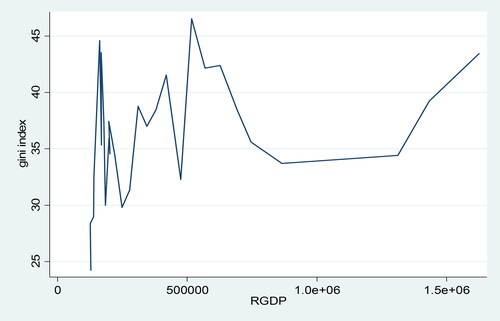
Figures 1 and 2 indicate the trends of the growth rate and inequality which are important variables and interests of our analysis. Ethiopia is one of the few fastest growing economies in the world, with a double-digit growth rate and RGDP with upward slopping and continuously increasing economic performance. However, the inequality of the county had a deterministic trend which moved up and down in different periods. As stated previously, one of the primary objectives of this study is to test the applicability of inverted “U” shape Kuznets hypothesis. To do this, we draw a line with RGDP on X-axis and the Gini index on the y-axis to specify the relationships between two main variables of the study.

Figure 1. Trends of real GDP.

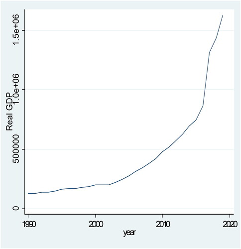
Figure 2. Trends of Gini index.

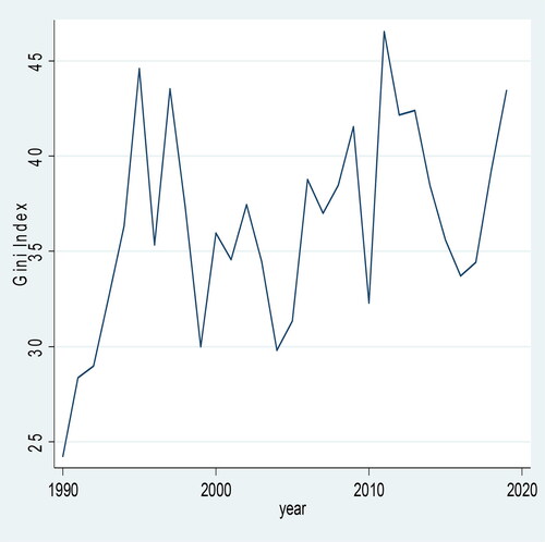
The central idea of the Kuznets curve is that there is a specific relationship between the growth of a given economy and income distribution level. It stated the presence of a high level of income inequality in the early stages of economic growth (the initial growth of the economy is accompanied by a high dispersion of income) but is negatively related at latter stages of growth. The increased GDP is expected to solve the problem of inequality, and the benefit from the growing economy will trickle down to the majority of the poor. However, when we tested for our country, there is a highly fluctuating Gini index with continuously increasing GDP (Figure 3) and we can say that there is no specific relationship between economic growth and income inequality in Ethiopia, at least for the period incorporated in this study, from 1992 to 2021.

Figure 3. Relationships between Gini index and economic growth.

4.2. Econometric analysis

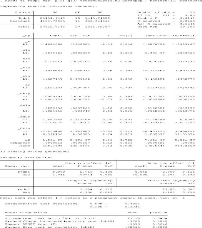
In this part of the study, the data analysis was conducted using the econometric concept of testing for stationarity. The relationship between the dependent and independent variables is determined using the estimation of the non-linear ARDL model and post estimation diagnostic test is applied to ensure that the relationship is meaningful. Before going to the estimation issue, the stationary test, which is an important aspect of time series analysis, must be considered using the Augmented Dickey-Fuller test, as shown (Table 3).

Table 3. The correlation matrix.

	Gini index	M2	Urban pop	RGDP	SSE
Gini index	1.0000
M2	−0.3644	1.0000
Urban pop	−0.5912	0.9111	1.0000
RGDP	−0.3763	0.9864	0.9206	1.0000
SSE	−0.0829	0.2782	0.4119	0.3303	1.0000

From the correlation matrix presented in Table 3, the Gini index is negatively correlated with all explanatory variables and highly correlated with urbanization as measured by a proxy variable of urban population growth rate and less correlated with education level as measured by secondary school enrolment. Beyond this, all explanatory independent variables are positively correlated each other and, the highest correlation exists between GDP and money supply (M2), while the lowest correlation exists between money supply and secondary school enrolment.

The Dickey-Fuller test serves as a checking procedure for the stationarity of variables by comparing the tau calculated with critical values to determine whether to reject the null hypothesis H₀ = the variables have unit roots. The decision rule states that the null hypothesis is rejected when the test statistics are greater than the tabulated values and the variable is determined to be stationary. In this study, the dependent variable Gini index was stationary at the level whereas the other variables were stationary at the first difference. The ‘non-linear’ ARDL model (Shimeles & Nabassaga, 2018) is applicable for variables that are integrated of different orders but I(0) and (1) and hence relevant or our analysis.

In addition to the stationary test, the bound test of co-integration is necessary to check for the presence of a true long-run relationship following (Pesaran et al., 2001). As seen from the Dickey-Fuller test above, all explanatory variables are non-stationary at level and we suspect to face the problem of spurious regression but the relationship is meaningful if the variables are co-integrated even when regressing the original data without any differences.

Then, after testing for co-integration (as presented in Table 4), it is possible to estimate the long-run model and the relationship between income inequality and its regressors is analyzed using the results from the non-linear ARDL model.

Table 4. Unit roots test for stationary.

Variables	Test statistics at level	Test statistics at difference	Dickey-Fuller Critical values			Stationary at
			1%	5%	10%
Gini	−3.818	–	−3.723	−2.989	−2.625	Level
Rgdp	3.253	−4.253	−3.730	−2.992	−2.626	1st difference
SSE	−0.585	−4.267	−3.736	−2.994	−2.628	1st difference
Urbpop	0.313	3.898	−3.736	2.994	2.628	1st difference
M2	−0.018	−6.029	−3.730	−2.992	−2.626	1st difference

Dickey-Fuller result obtained from stata using dfuller command.

As shown from the Appendix A and the Table 4, the coefficient of determination of the ‘non-linear’ regression model is given by 0.85, which means that out of the total change in Gini coefficient, 85% is determined with in the model by the joint effect of explanatory variables, the same result as (Lakner et al., 2021). Additionally, post estimation diagnostic tests were considered, and no violations were detected for the data set. With the null hypothesis of H₀: there is homoscedastic variance for heteroskedasticity, H0: there is no omitted variable for model specification and H₀: the error term is normally distributed for normality, we fail to reject with respective probabilities of 0.3245, 0.9046 and 0.9868 similar to Alemayehu et al. (2008).

The long run significance of variables is tested using the t-value, and hence variables with greater than two in absolute terms are said to be statistically significant (using rule of thumb), The deterministic variables of urban population and money supply as well as increasing aspects of human capital are statistically insignificant, as stated in Shimeles and Nabassaga (2018). The lagged value of Gini index is negatively related to the current inequality(1% rise in Gini index in past year will lead to lowering it by .46% today), and this may be the result of government actions to correct the widening income gap to agree the idea raised. The most important variable in the study was economic growth, measured by the RDGP growth rate. Both the increasing (RGDP+) and decreasing (RGDP-) parts of the economy have no similar effects on inequality. The result from the ‘non-linear’ ARDL model shows that inequality increases by .0001986 when GDP rises by unity while it will skyrocket by 0.194 due to a unit fall of the RGDP as raised by Abebe (2016). This is the reason why we preferred the non-linear model rather than the linear model because it may be an asymmetric effect of on variable by rejecting the null hypothesis of $\frac{{{\theta }_i}^{+}}{{\beta }_1}$ =$\frac{{({\theta }_i}^{\_}}{{\beta }_1}$. When GDP increases in the Ethiopian economy, income inequality increases at the highest percentage, which has the economic implication of an unfair personal income distribution. Few private business owners and some corrupt government officials are taking all the increased advantages and the benefit is not trickling down to the majority of the poor, and that is why increased GDP is associated with the highest rise in income inequality.

The remaining variable affecting the Gini index in the long run (as shown in Appendix A) is the reducing part of human capital as measured by a proxy variable of secondary school enrolment (Marrero & Servén, 2018). As shown in the estimation results (Table 5), increasing the number of students enroled in secondary schools is unrelated to the Gini coefficient in Ethiopia. In the nation, education does not solve the inequality problem because less attention is paid to professionals who spend the majority of their lives in schooling, which agrees with the results of Sehrawat and Giri (2018), Tassew et al. (2009), and Van der Weide and Milanovic (2018). Almost all professional workers, including those with PhD degrees are paid a small amount of money when compared to the income of individuals engaged in their own businesses. Why the reducing part of SSE enrolment had the power to reduce (Alemayehu et al., 2008) the inequality is that those dropouts are engaging in private jobs and hence can share the benefit that was taken by few deem-rich individuals (Appendix A).

Table 5. Bound tests for non-linear co-integration.

Null Hypothesis H0: no long run relationship Decision: reject H0 if p value < 5%	F-statistics	Prob > F	Lower bound	Upper bound	Conclusion
	3.80	0.0149	4.428	6.250	Co-integrated

N.B: rejecting the null hypothesis (with p < 5%) means there is true long run relationship even with asymmetry. A Narayan (2005) F-critical value for a small sample size was used and the null hypothesis was rejected because the statistics were not between the upper and lower bounds.

Table 6. Long run estimation of non-linear ARDL model.

Variables	Coefficients	St. error	t-value	p-value	CI
Const.	458.3808	129.8674	3.53	0.005	172.5446 744.2169
Gini	−.4623082	.1932623	−2.39	0.036	−.8876758 −.0369407
Rgdp^+	.0001986	.0000899	2.21	0.049	6.39e-07 .0003965
Rgdp^-	.0194041	.0056107	3.46	0.005	.0070551 .0317532
SSE^+	.7928663	3.046033	0.26	0.799	−5.911406 7.497139
SSE^-	−4.627437	2.191162	−2.11	0.058	−9.450151 .1952775
M2	−1.08e-07	2.99e-07	0.36	0.725	−7.66e − 07 5.50e − 07
Urbanpop	| −.0000213	.0000187	0.281	−1.13	−.0000625 .00002
R-squared = 0.8468 F (16, 11) = 3.80 Prob > F = 0.0149	Portmanteau test up to lag 12 (chi2) 21.28 0.0464 Breusch/Pagan heteroskedasticity test (chi2) .9706 0.3245 Ramsey RESET test (F) .1836 0.9046 Jarque-Bera test on normality (chi2) .02665 0.9868

Variables with p-value less than 5% are statistically significant.

The relationship between the dependent and independent variables analyzed previously was all about the long-run but did not indicate the short-run relationship, hence, it is necessary to develop a short-run error correction model by incorporating the value of variables at different (Appendix A).

In the short run, the only variable that had the power to affect the level of income inequality as measured by the Gini coefficient (Table 7) was the falling part of RGDP. In contrast to with the findings of Shimeles and Nabassaga (2018) and (Kararach, 2022), in this study, income inequality is increased with in line with failing part of economic growth since majority of individuals became income less while the economy is at recession (1% reduction in RGDP is associated with rise in Gini index by 0.022). This result is similar to that of Kararach (2022), Lakner et al. (2020), and Lakner et al. (2021).

Table 7. Long run and short run asymmetry test.

Exogenous variables (with non-linear relationships)	Long run asymmetry		Short run asymmetry
	F-statistics	P > F	F-statistics	P > F
RGDP	2.984	0.012	13.85	0.003
SSE	6.906	0.023	2.286	0.159

The long-run analysis we conducted considers the asymmetric relationship between the increasing and decreasing parts of real gross domestic product and secondary school enrollment. The asymmetric test with the null hypothesis of no asymmetry (H₀:${{\theta }_i}^{+}={{\theta }_i}^{-}$) is rejected by considering the probability value given in Table 6.

As presented in Table 5, the dynamic multipliers of the Non linear ARDL model show the cumulative effect of RDGP and SSE on income inequality for 30 years time horizon. As depicted in Figure 4, an increase in secondary school enrolment has a negative effect on the Gini index while the rising part of the SSE positively affects the Gini index. Additionally, the cumulative effect f RDGP on the Gini index is positive whereas a decrease in RGDP has a temporally negative effect on income inequality as measured by the Gini index (Table 8).

Figure 4. The dynamic cumulative effect of RGDP and Secondary School enrolment on Gini index.

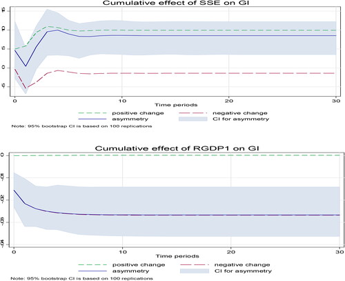
Table 8. Error correction model non-linear ARDL estimation.

Variables	Coefficients	Std.errors	t-values	p > t	CI
$\Delta$ Gini	−.0551321	.2090794	−0.26	0.797	−.5153128 .4050485
$\Delta$ Rgdp^+	.0000703	.0000798	0.88	0.397	−.0001053 .0002458
$\Delta$ Rgdp^−	.0229956	.0055263	4.16	0.002	.0108322 .035159
$\Delta$ SSE^+	1.562755	2.247469	0.70	0.501	−3.38389 6.5094
$\Delta$ SSE^−	−1.455496 -	2.249865	−0.65	0.531	6.407415 3.496424
Const.	458.3808	129.8674	3.53	0.005	172.5446 744.2169

N.B: $\Delta$ is to mean the first deference of time series variables to consider short run relationships.

5. Conclusion and recommendations

This study analyzes economic growth and income inequality in Ethiopia with special emphasis on identifying the relationship between inequality and economic growth in Ethiopia. Using time series data from 1992 to 2021, the applicability of inverted “U” shaped Kuznets hypothesis is tested and there is no specified relationship between income inequality and economic growth in opposite to Kuznets idea which states the presence of high gini index when growth starts but finally fails with rise in economic growth at final stages.

The ‘Non-linear’ ARDL model is applied to identifying the determinants of income inequality by using the Gini index as a measure of personal income inequality and real GDP, secondary school enrolment, number of urban population and money supply as explanatory variables. The estimation result of the ‘non linear’ ARDL model shows that failure in GDP is associated with a higher increment in the Gini index than the rising part of GDP. This means that the Gini index is increases when, GDP increases and decreases. However, the rate of increment in income inequality is higher when the GDP is decreases. Thus, a high level of income inequality is experienced in the depression stage but it can be reduced when the economy is in recovery.

Additionally a reduction in secondary school enrollment leads to a reduction in income inequality in contrast to the theoretical power of education to reduce income inequality, as first explained by Bound and Johnson (1992). This means that individuals with high education level are paid less and those school dropouts are able to share national income when compared with individuals who completed their schooling.

Using the estimation results of our model, we suggest two basic policy recommendations for solving the problem of income inequality in Ethiopia. The first one is related to promoting economic growth, as the depression of the economy resulted in high income inequality. To do this, the government shall apply an expansionary fiscal policy by increasing government expenditure and reducing taxes since expansionary fiscal policy has a positive distributional impact on income as presented by the International Monetary Fund (2015). Second, education is becoming ineffective in reducing income inequality but school dropout is important in reducing inequality. This result may be related to the less responsive action of the government, which discourages individuals with education by making low payments; therefore, the government had better to revise the country’s income policy; educated individuals must be paid sufficient income equivalent to their qualifications and a favorable working environment is needed to make the intellectuals to accumulate their own wealth to minimize income inequality.

The limitation of this study is the limited access to secondary time series data, which obliged the researchers to fix the year of study, between 1992 and 2021 only. We recommend that researchers who want to investigate more in this area include the effect of Ethiopian internal conflicts started in 2021 on its economy and its effect on widening or narrowing income inequality among Ethiopian citizens by including more years to expand the time span of the study period.

Author’s contribution

Both authors equally participate in this work.

Abbreviation
CSA	=	Central Statistical Authority
GDP	=	Gross Domestic Product
IMF	=	International Monetary Fund
MoFEC	=	Minister of Finance and Economics Cooperation
NBE	=	National Bank of Ethiopia
NARDL	=	Non-Linear Auto Regressive Distributed Lag Model
WB	=	World Bank

Disclosure statement

No conflict of interest between authors.

Data availability statement

The data used for this finding are on the hands of the principal researcher and I can provide it to editors when needed.

Appendix A:

Estimation of the NARDL model

References

- Abebe, F. (2016). Determinants of income inequality in urban Ethiopia: a study of south wollo administrative zone, Amhara national and regional state. International Journal of Applied Research, 2(1), 1–14.
- Afonso, C. (2008). Determinants of income distribution and efficiency of public spending in Bangladesh. Working Paper Presented to Bangladesh Institute of Economics, vol. 10(2), p. 52.
- Alemayehu, G., Abebe, S., & John, W. (2008). Growth, poverty and inequality in Ethiopia: Which way for Pro-Poor Growth? Journal of International Development, 21, 947–970.
- Barro, R. J. (2000). Inequality and growth in a panel of countries. Journal of Economic Growth, 5(1), 5–32. https://doi.org/10.1023/A:1009850119329
- Belay, Z. T. (2023). The determinates of income inequality in urban Ethiopia: the case of KoboTown. Developing Countries Study, 13(1). https://doi.org/10.7176/DCS/13-1-01
- Bound, J., & Johnson, G. (1992). Changes in the structure of wages 1980’s: an evaluation of alternative explanations. American Economic Review, 82(3), 371–392.
- Ephrem, I. (2006). Analysis of economic growth, income inequality and poverty using CGE model. MSc thesis presented to graduate studies of Addis Ababa University, Addis Ababa.
- Fuwa, S. (2003). Growth and redistribution: is there a trickle down effect in Philippines. Discussion no. 2002-2, Philippines institute for development.
- International Monetary Fund. (2015). Annual report.
- Kaldor, N. (1955). Alternative theories of distribution. The Review of Economic Studies, 23(2), 83–100. https://doi.org/10.2307/2296292
- Kararach, A. G. (2022). Disruptions and rhetoric in African development policy. Routledge.
- Kuznets, S. (1955). Economic Growth and Income Inequality. The American Economic Review, 45(1), 1–28.
- Lakner, C., Gerszon Mahler, D., Negre, M., & Beer Prydz, E. (2020). How much does reducing inequality matter for global poverty? Global Poverty Monitoring Technical Note 13, World Bank, Washington, DC.
- Lakner, C., Yonzan, N., Mahler, D., Castaneda, R., & Wu, H. (2021). Updated estimates of the impact of COVID-19 on global poverty: looking back at 2020 and the outlook for 2021. https://blogs.worldbank.org/.
- Maina, K. (2006). The relationship between economic growth and the applicability of Kuznets curve in Kenya.
- Marrero, G. A., & Servén, L. (2018). Poverty, inequality and growth: a robust relationship? Policy Research WP Series 8578, World Bank.
- MoFEC. (2006). Ethiopia: plan for accelerated and sustained development to end poverty. Addis Ababa Ethiopia.
- Nayaran, P. K. (2005). The saving and investment nexus in China: evidence from emerging market. Energy Economics, 37(17), 1979–1990.
- Okidi, U. (2004). Understanding basic determinants of income inequality in Uganda. M.Sc thesis presented to graduate studies of Makerere University.
- Oliver, G. (2010). Functional distribution of income inequality and incidence of poverty. Working paper, no.58, University of Texas.
- Perdiz, A. (2010). World growth and inequality. Journal of International Economics, 2, 10–57.
- Pesaran, M. H., Shin, Y., & Smith, R. J. (2001). Bounds testing approaches to the analysis of level relationships. Journal of Applied Econometrics, 16(3), 289–326. https://doi.org/10.1002/jae.616
- Sehrawat, M., & Giri, A. K. (2018). The impact of financial development, economic growth, and income inequality on poverty: evidence from India. Empirical Economics, 55(4), 1585–1602. https://doi.org/10.1007/s00181-017-1321-7
- Shimeles, A., & Nabassaga, T. (2018). Why is inequality high in Africa? Journal of African Economies, 27(1), 108–126. https://doi.org/10.1093/jae/ejx035
- Shin, Y., Yu, B., & Greenwood-Nimmo, M. (2014). Modelling asymmetric cointegration and dynamic multipliers in a nonlinear ARDL framework. In R. Sickels, & W. Horrace (eds.), Festschrift in Honor of Peter Schmidt: Econometric Methods and Applications (pp. 281–314). Springer.
- Tassew, W., Hoddinott, J., & Dercon, S. (2009). Poverty and Inequality in Ethiopia. Addis Ababa University, International Food Policy Research Institute and University of Oxford, Addis Ababa Ethiopia.
- Ullah, S., Chishti, M. Z., & Majeed, M. T. (2020). The asymmetric effects of oil price changes on environmental pollution: evidence from the top ten carbon emitters. Environmental Science and Pollution Research International, 27(23), 29623–29635. https://doi.org/10.1007/s11356-020-09264-4
- UNDESA. (2009). Income distribution and economic growth in sub-Saharan African countries. Working paper in economics.
- Van der Weide, R., & Milanovic, B. (2018). Inequality is bad for growth of the poor (but NOT FOR THAT OF THE RICh). The World Bank Economic Review, 32(3), 507–530. https://doi.org/10.1093/wber/lhy023
- Wan, H. (2006). Inequality growth nexus in China. Beijing Economic Journal, 15, 12–20.