Empirical investigation on the dynamics effects of population and economic growth in Ethiopia: an application of the VEC model

Abstract

Most of the previous economic theories and empirical studies revealed that the relationship between population and economic growth is controversial and inconclusive in different parts of the world. However, previous studies have attempted to examine the relationship between population and economic growth, but their results have been vague or not even sufficiently realistic to address the issue practically. Thus, cognizant of this fact, this study investigates the dynamic effect of population and economic growth in Ethiopia. This study used a Vector Error Correction Model (VECM) and estimated using annual data for the period 1991-2022. The study found that, in the short run, high population growth was associated with increases in real gross domestic product. However, in the long run, population expansion hurts economic growth. Furthermore, the analysis shows that there is no causal relationship between population growth and economic growth by using block exogenity test. In conclusion, population growth has a greater short term positive impact on economic growth than it does in the long term. This study suggests that the government should adopt a pro-natal strategy that uses incentives for agricultural output in the short term to encourage individuals to have more families; the government should promote anti-natal policies to sustain economic growth that encourages individuals to have fewer children in the long run. Additionally, instead of solely focusing on population growth, the study suggests that the government prioritize and sustain economic growth by centralizing and improving the real money supply.

IMPACT STATEMENT

Economic growth is the one and the main concern of the macroeconomic goal of the nation because it is vital in reducing the poverty level, creating employment opportunities, and narrowing the inequality gap. Hence, population growth is a main concern variable on the issue of determines economic growth. Even though there are many studies conducted in different countries including Ethiopia, population in terms of promoting economic growth; the detail dynamics effects of population and economic growth in terms of addressing the problem and practical issue is still questionable and inconclusive. To address these conflicting ideas the paper fills the gap in the literature by developing a quantitative macroeconomic model that captures the dynamic effects of population and economic growth in Ethiopia. Thus, the researcher tried to do so.

Keywords:

• Population
• VECM
• economic growth
• Ethiopia

Reviewing Editor:

• George Mudimu, Development Sciences, Marondera University of Agricultural Sciences and Technology, Marondera, Zimbabwe

Subjects:

• Development Policy
• Economics and Development
• Population & Development
• Economics

1. Introduction

High population growth remains a controversial topic worldwide. There has been a periodic increase in the global population. Currently, the world population reaches to more than 8 billion people in 2023. In addition, Africa will have more than 1.46 billion people in 2023 (World Bank open data, 2023) Moreover; Ethiopia’s population is predicted to exceed 120 million by 2023, and the population of Ethiopia will be 123,379,924 in 2022 (World Bank open data, 2023).

As more people ultimately consume more of the Earth’s finite resources, population expansion has been and will continue to be troublesome, slowing down long-term growth (Linden, 2017). Most developing countries, including Ethiopia, have a strong population growth rate but a poor GDP growth rate when compared to the preceding time. The central emphasis of a country’s macroeconomic policy is economic growth. It is still uncertain whether population and economic growth are related. Thus, different economic theories have arisen because of economist’s divergent views on population expansion and economic growth. The optimistic viewpoint claims that population growth (urbanization) spurs technological acceleration and contributes to capturing the economic scale (Boserup, 1965; Khan et al., 2022; Simon, 1977; Zahoor et al., 2022), whereas the pessimistic view claims that population growth harms economic growth by lowering savings and investments (Coale & Hoover, 1958; Yahaya, 2019; Yang & Khan, 2022).

Consistently, high fertility rates and rapid population growth hurt the economic and social development of less developed nations, which is a barrier to development because it puts pressure on budgeted expenditures for services, housing, and education (Coale & Hoover, 1958; Dennis & Robert, 2008). Similarly,(Assefa, 1994) noted that even though population growth is not the primary reason for poor standards of living in developing nations, it exacerbates the issue of underdevelopment and renders development opportunities impossible.

Ethiopia had a population of 49,609,969 in 1991 and was growing at a 3.5% annual pace. The outcome has changed from 66,224,804 in 2000 to 87,639,964 in 2010, 100,835,458 in 2015, 114,963,588 in 2020, and 117,876,227 in 2021 and 123,379,924 in 2022 with the corresponding yearly growth changes of 2.8%, 2.8%, 2.57%, and 2.53% and 2.57%. More than 120 million people live in Ethiopia, which has a growing population. Due to its rapid population growth dependent on rain-fed agriculture and the harmful effects of climate change, Ethiopia is particularly vulnerable to the twin threats of poverty and deterioration of natural resources. Ethiopia’s population is growing rapidly, possibly as a result of the three most important factors: a high birth rate, a low mortality rate, and rising net migration. However, economic development does not keep pace with population increase. Concerning population growth, Ethiopia’s 2019/20 annual GDP growth rate of 6.1% was unsatisfactory. The nation also faced several economic issues, including high unemployment and inflation rates of 21.6%, and 20%, respectively (National Bank of Ethiopia, 2021/2022; World Bank open data, 2023).

Therefore, population growth determines a nation’s economic development, and it is necessary to study Ethiopia’s growing population. The dynamics of Ethiopia’s population growth and economic growth are still debatable for researchers, there is limited literature on the nation, and their findings are inconclusive as well. As a result, his study seeks to bridge the gap by providing an empirical investigation into the dynamic effects of population growth on economic growth in Ethiopia and their presence and direction of causality between them. The country, being a low-income nation with a rapidly expanding economy and a rapidly growing labour force and population, presents a compelling context for such an analysis.

Although many empirical studies have examined the relationship between population and economic growth in different regions of the world, very few studies have been conducted on Ethiopia. Some studies conducted in Ethiopia, such as those by Abayneh & Belay (2015), Terefe (2018), Wuletaw (2018), Adisu (2019), and Kidane (2020), have explored the relationship between population and economic growth. These studies have yielded different findings. First, some have indicated a positive impact of population growth on economic growth, as observed in the works of Wuletaw (2018), Kidane (2020), Sibe et al. (2016), Okunolа et al. (2018), Mohsen & Chua (2015). Conversely, others have found a significantly negative influence of population growth on economic growth, as demonstrated by Terefe (2018), Adisu (2019), Akintunde & Oladeji (2013), and Anudjo (2015). Consequently, the dynamic relationship between population and economic growth remains a major controversial issue in economic discourse globally, with inconclusive findings in the empirical literature. Therefore, further research is needed to address this issue comprehensively.

Second, many previous studies (e.g. Abbasi et al., 2021; Adisu, 2019; Kidane, 2020) conducted in time series were conducted using ARDL. For example, Auto Regressive Distributed Lag is more flexible than Vector Auto Regressive or Vector Error Correction Model (VECM) in terms of stationarity for I(0) and I(1). However, stationarity is a necessary condition for estimating cointegration and error correction methods and is important for checking the accuracy and adequacy of the data. In addition, the regression of non-stationary variables often leads to problems with spurious regressions, and variables only have contemporaneous relationships rather than full causality (Granger & Newbold, 1974; Harris & Sollis, 2003). Therefore, taking stationarity with the ARDL model does not guarantee data quality and assurance, so this flexibility leads to incorrect inferences and wrong conclusions, and undermine the overall robustness of the findings. To address these concerns and ensure a more rigorous analysis, this study adopts the Vector Error Correction Model (VECM) instead. By employing the VECM, the study aims to mitigate the potential issues associated with spurious relationships and to provide more reliable and meaningful insights into the real problem at hand.

Third, many previous studies (e.g. Abbasi et al., 2021; Adisu, 2019; Wuletaw, 2018) have not examined the effects of the dynamics of population growth and key macroeconomic variables such as real GDP, external debt-to-GDP ratios, real money supply, and inflation, which are commonly used to measure economic growth. Many economists argue that real GDP provides a more accurate measure of economic growth compared to nominal values (e.g. Barro, 1995; Mankiw, 1998). Hence, in this study, real GDP is employed as the measure to assess economic growth. Furthermore, the study investigates the relationship between population and economic growth by examining their relations with real money supply and the ratio of external debt to GDP. By considering these macroeconomic variables, the analysis aims to offer a comprehensive understanding of the dynamics between population and economic growth in a more realistic and meaningful context.

Finally, many of the previous researchers did not utilize recent data, while this study used the most recent and covered the longest period. Therefore, this study tried to fill the above knowledge gaps, examine the dynamic effects of population growth and economic growth and their presence and direction of causality between them from 1991 to 2022. Thus, to capture the details of these dynamics, the study employs the Vector Error Correction Model (VECM), which allows for the analysis of both short term and long term effects between population and economic growth. By employing recent data and employing a comprehensive analytical approach, this study aims to provide valuable insights into the dynamics relationship between population growth and economic growth.

2. Literature

It is important to properly study, monitor, and control population growth rates. If not, it might undermine once again all of the government’s attempts to fulfill its plan to increase the standard of living and quality of life for everyone in the nation. The argument between population and economic growth has not been recent. Malthus (1798) asserted that productivity rises arithmetically whereas population grows geometrically. Therefore, there is disagreement about whether population growth affects economic growth in least-developed countries.

Overpopulation causes soil erosion, deforestation, and other uses of natural resources as well as a limited supply of land resources. A key problem in development is the production of sufficient food for a large population. In addition to its slow economic growth, Ethiopia faces several problems, such as a shortage of available land, starvation, drought, and outdated technologies. A vicious circle of problems, such as excessive unemployment, poverty, inflation, and a lack of foreign currency have also kept the country trapped (IMF, 2020 report).

Consistently, Dyson (2010) noted that a reduction in mortality benefits economic growth, which improves the standard of living. People tend to think more about the future, are more willing to take risks, and become inventive as they age. According to research by Bloom & Canning (2001) and Kalemli-Ozcan (2002), a decrease in mortality tends to boost educational attainment and saving rates, which, in turn, leads to an increase in investments in both physical and human capital. Besides, Malthus (1798) emphasized the negative effects of high rates of population growth on savings and investment, and hence, future growth, as well as the barriers to growth represented by diminishing returns. A rising population necessitates a greater allocation of scarce resources to consumption rather than investment. Another factor that favors the gloomy view is resource depletion. Rapid population growth signals an expanding labor force. A sizable share of young people in the workforce could promote technical advancement and economic expansion owing to their increased adaptability and mobility. Figure 1 provides a summary of the relationship between population and economic growth. Thus, the summary entails that population has both a negative and positive impact on economic growth (Boserup, 1965; Khan et al., 2022; Kremer, 1993; Malthus, 1798; Yahaya, 2019; Yang & Khan, 2022).

Figure 1. Summary of the relationship between population and economic growth.

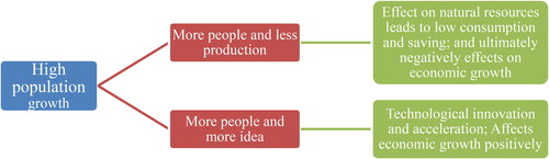
The above theoretical framework can be used to summarize the many research suggestions about the relationship between population growth and economic growth: there is a theoretical literature view in both pessimistic and optimistic views that supports population control policy, especially in developing countries, while optimistic views do not support population control policies, because population growth leads to increased labor productivity, per capita income, and improvement in living conditions (Boserup, 1965; Kremer, 1993).

When adopting the ordinary least squares approach, population growth had a positive influence on Nigeria’s economic development from 1980 to 2010 (Tartiyus et al., 2015). In addition, using the ARDL technique for the years 1982 to 2016, population expansion in Nigeria has a favorable effect on food production both in the short and long term (Okunolа et al., 2018). Population growth hinders economic growth both immediately and in the long term. However, using the ARDL model from 1981 to 2018, economic growth in Ethiopia had a favorable effect on population growth (Adisu, 2019). Furthermore, Mohsen & Chua (2015) used the VAR approach to analyze whether Syria’s population growth had a beneficial influence on economic growth from 1980 to 2010. Besides, urbanization (population growth) is positively associated with the ecological footprint and economic growth in the selected Organization for Economic Co-operation and Development (OECD) countries (Khan et al., 2022).

Using the ARDL approach, Barbados’ population growth and density have a positive and substantial impact on economic growth, while economic growth hurts population growth and international migration on economic growth (Mamingi & Perch, 2013). In addition, (Wuletaw, 2018) looked at whether agricultural output and population growth increased over time. Even though land degradation and population increase were two of the biggest development issues from 1985 to 2016, productivity growth exhibited erratic tendencies in comparison to population growth. Moreover, using the ECM approach, the 30 most populous nations showed a long term positive association between population growth and economic development from 1960 to 2013(Sibe et al., 2016). Furthermore, in the short run, urbanization population growth has a positive effect on economic growth in Pakistan by using a novel dynamic ARDL model, and urbanization is positively related to carbon dioxide emission and economic growth in China respectively (Abbasi et al., 2021; Zahoor et al., 2022). Besides, population growth has a positive effect on carbon emissions (Wang et al., 2023).

By augmenting a VAR model covering 1963 to 2009, Thuku et al. (2013) discovered that population growth has a positive influence on economic growth and, presumably, economic development in Kenya. In addition, using the ARDL technique for the years 1982 to 2016, population expansion in Nigeria has a favorable effect on food production both in the short and long term (Okunolа et al., 2018). However, using the VECM from 1952 to 1984, population size had a negative influence on China’s economic growth (Yao et al., 2013). Moreover, using Johanson’s co-integration, population growth did not influence per capita income growth in India from 1950 to 1993 (Dawson & Tiffin, 1998). While, by using the threshold regression model spanning from 1996 to 2015, population aging and urbanization have improves the quality of the environment and economic growth in the selected countries 134 countries (Wang et al., 2022). In addition, Sadiq et al. (2023) found that mitigating climate change has been facilitated by the consumption of renewable energy and the control of corruption; nevertheless, policy uncertainty hinders the efforts of BRICS-1 countries to reduce CO2 emissions. Furthermore, as long-term economic growth increases, CO2 pollution decreases continuously, supporting the EKGC theory for these countries. Lastly, corruption control and economic growth have a bidirectional causal relationship with renewable energy, but policy uncertainty has a unidirectional relationship with CO2 emissions by using the panel cross-section ARDL model and D-H causality method from the period 1990 to 2020 in BRICS-1 nations. Moreover, (Terefe, 2018) concluded that economic growth interacts negatively with unemployment, the total fertility rate, child mortality rates, and population growth. Similarly, rapid population growth hurts the economic growth of sub-Saharan African nations, as evidenced by the top ten manufacturing countries respectively (Akintunde & Oladeji, 2013; Khan et al., 2021). Furthermore, population expansion in Ghana’s economy has a negative influence on economic growth in the near term and a long-term, unidirectional causal relationship between them when employing the ARDL model for the period 1980 - 2013 (Anudjo, 2015). Besides, using the ARDL model for 1980 to 2014, population growth accelerated environmental deterioration in Nigeria in both the short and long terms and population growth deteriorates environmental sustainability in the long run evidenced by thirty International Energy Agency member countries respectively (Yahaya, 2019; Yang & Khan, 2022). While, population growth improved environmental quality as evidenced by comparative analysis in Australia and the Global sample (Zakari et al., 2023).

3. Methods

3.1. Data description

This study is based on macroeconomic data spanning the years 1991–2022 to empirically evaluate the short run and long run effects between population growth and economic growth in Ethiopia. The choice of the period is based on the availability of data for the main variables of the paper, and there was a regime change, economic policy, and strategy change in 1991. As a result, this study covers the transitional period till 2022. Table 1 shows that relevant data were collected from the Ministry of Finance and Economic Development (MOEFD), Ethiopian Economic Association (EEA), National Bank of Ethiopia (NBE), and World Bank (WB).

Table 1. Variable description.

Variables^1	Description	Source	Expected sign
RGDP	The monetary value of Real Gross Domestic Product at basic year price which measures economic growth	National Bank of Ethiopia (NBE), EEA	Economic growth is best measured by real GDP than nominal GDP (eg. Mankiw, 1998; Barro, 1995). As a result, this study uses RGDP measured in Ethiopian currency.
PG	It is the total number of people increases in a country and a given period.	World Bank	PG has a positive, negative, and neutral effect on Economic growth (Malthus, 1798; Boserup, 1965; and neutralist argument). Therefore, this study also expects negative signs.
MS/P	Real money supply at a period in Ethiopia	National Bank of Ethiopia (NBE), EEA	Money supply has an importance on economic growth. This is supported by many monetarist views (Chaitip et al., 2015). Hence, this study also expects positive signs.
ED/GDP	External debt to gross domestic product ratio at a period	National Bank of Ethiopia (NBE), MOFED report	ED/GDP harms economic growth (Teklu et al., 2014). Thus, this study expects a negative sign.
INF	The average increase in price in a year	National Bank of Ethiopia (NBE), MOFED	Inflation is one macroeconomic variable that determines growth and can be considered a curse for economic growth. (Khan & Naushad, 2020 in World Economy). As a result, this study also expects negative signs.

3.2. Analytical framework

The Solow Swan model of economic growth, which stipulates that saving rate, population growth, and technology are supplied, is used in this study. It is derived from the following theoretical framework and several other studies. The model encompasses two inputs, capital and labor, which are compensated according to marginal productivity (Solow, 1956).

Consider that a Cobb-Douglas production function at time t can be calculated as follows; (1) $$Y\left(t\right)={K\left(t\right)}^{\beta }A\left(t\right){L\left(t\right)}^{1-\beta },0<\beta <1$$(1)

Where Y is output, K is capital, A is the level of technology, L is labor, and the starting levels of capital, labor, and technology are taken as provided. Both the labor force and technological advancements are growing steadily. Thus, $\frac{\mathit{\text{dL}}}{\mathit{\text{dt}}}=\mathit{\text{nL}}\left(t\right)$, and:$\frac{\mathit{\text{dA}}}{\mathit{\text{dt}}}=\mathit{\text{gA}}\left(t\right)$ where n and g are exogenous parameters and d denotes the derivative, are true.

The variable growth rate is equal to the rate of change of its log, which demonstrates that the rate of change of the logs of L and A is constant and equal to n and g respectively, and is added to the above equation using natural logarithms. Thus, L(0) and A(0) represent the value of labor and technology at time zero, respectively, and as a result, $\mathrm{\text{ln}}\hspace{0.17em}L\left(t\right)=(\mathrm{\text{ln}}\hspace{0.17em}L\left(0\right))+\mathit{\text{nt}}$, and $\mathrm{\text{ln}}\hspace{0.17em}A\left(t\right)=(\mathrm{\text{ln}}\hspace{0.17em}A\left(0\right))+\mathit{\text{gt}}$. Additionally, using the exponential function for the two sides of the equation, the following result is obtained: (2) $$L\left(t\right)=L\left(0\right)e^{\mathit{\text{nt}}}$$(2) (3) $$\mathrm{A}\left(\mathrm{t}\right)=\mathrm{A}\left(0\right){\mathrm{e}}^{\mathrm{\text{nt}}}$$(3) $A\left(t\right)L\left(t\right)$ Refers to the number of effective units of labor growing at a rate of $n+g$.

The Solow model assumes that a constant fraction of output s is invested in. By definition: $k=\frac{K}{\mathit{\text{AL}}}$ is the stock of capital per effective unit of labor, and $y=\frac{Y}{\mathit{\text{AL}}}$ is the level of output per effective unit of labor. The evolution of capital per effective unit of labor is explained by: (4) $$\frac{\mathit{\text{dk}}}{\mathit{\text{dt}}}=\mathit{\text{sy}}\left(t\right)-\left(n+g+\delta \right)k\left(t\right)$$(4)

Which is equal to $s{k(t)}^{\beta }-\left(n+g+\delta \right)k\left(t\right)$, and at steady-state $\mathit{\text{dk}}$ obtained as $s{\mathit{\text{dk}}}^{\beta }=\left(n+g+\delta \right)\mathit{\text{dk}}$. More specifically, $\mathit{\text{dk}}=({\frac{s}{n+g+\delta })}^{\frac{1}{1-\beta }}$ indicates that $k$ converges to the steady-state value $\mathit{\text{dk}}$ and $\delta$ refers to the depreciation rate.

Therefore, from the above equation, the steady-state capital-labor ratio and saving rate are positively related, but negatively related to population growth (Thuku et al., 2013). The main prediction of the Solow model considers the effects of savings and population growth on real income. Hence, to find the steady-state income per capita, substitute the last equation by applying the substitution method in the production function above, and taking the natural logarithm gives us: (5) $$\mathit{\text{ln}}\left[\frac{Y\left(t\right)}{L\left(t\right)}\right]=\mathit{\text{lnA}}\left(0\right)+\mathit{\text{gt}}+\frac{\beta }{1-\beta }\mathrm{\text{ln}}\hspace{0.17em}\left(s\right)-\frac{\beta }{1-\beta }\mathrm{\text{ln}}\hspace{0.17em}\left(n+g+\delta \right)$$(5)

It predicts not only the sign but also the size of the coefficients of saving and population growth because production factors are compensated for by their marginal productivities in this model. Finally, the link between economic and population growth can be deduced using theoretical methods.

3.3. Econometrics model specification

This study specifies the econometric model following the works of (Asteriou & Hall, 2011; Ayanaw, 2020; Calderón & Fuentes, 2013; Tasew, 2011; Thuku et al., 2013). The term ‘stationary data’ in time series econometrics refers to data whose mean, variance, and covariance remain constant during observation. Auto-regressive random process-generated Y_t time series (taking AR(1) as an example) Model: If ${ Y}_t=\delta Y_{t-1}+{\epsilon }_t$, then

• If $\delta$<1, the data are stationary.

• If $\delta$>1, then the series (Y_t) explodes. The data were non-stationary if $\delta$ =1.

A common technique for determining whether a variable is stationary is the augmented Dickey-Fuller test (Dickey &Fuller, 1979). Since ADF is important to avoid residual autocorrelation, it includes the lagged first difference of the dependent variable which is vital. Various researchers have employed ADF, including (Ayanaw, 2020; Ogundipe et al., 2013; Udemba, 2020).

The general equation of ADF, which contains constant and delayed differences, is: (6) $${\Delta y}_t=a+{\mu }_t+\left(\delta -1\right)y_{t-1\mathrm{ }}+\sum _{i=1}^p{\gamma }_i\Delta y_{t-1}+{\epsilon }_t$$(6)

If $\left(\delta -1\right)=0$, there is a non-stationary (unit root problem) in the null hypothesis ($H_0:\delta =1$) against the alternative hypothesis if $\left(\delta -1\right)<0,$ there is stationary that is $(H_1:\delta <1)$.

3.3.1. Cointegration

In the time series analysis, Cointegration among the variables shows the presence of long run relationships in the system. That is cointegration among the variables shows the presence of long-run relationships among the non-stationary variables in the system. Cointegration is characterized by two or more variables in I(1) which shows a common long run economic relationship. Cointegration in VAR, suppose the K variables Y₁, Y₂, ……, Yk collected in the vector Y am I(1), m in such a case, there will be no cointegration at all or there exists one or two up to k-1 linearly independent co integration vectors (Ayanaw, 2020).

The elements of a k-dimensional vector Y are cointegrated of order (d,c) and, Y ∼ CI(d, c) if all elements of Y are integrated of order d, I(d), and if there exists at least one non-trivial linear combination z of these variables, which is I(d−c), where d, c > 0 holds, that is if and only if ß’Y_t = z ∼ I(d−c). Vector ß is denoted as an integration vector. The cointegration rank r is equal to the number of linearly independent co-integration vectors. The cointegration vectors are the columns of the cointegration matrix B, with B’Y_t = Z_t (Ayanaw, 2020; Engel & Granger, 1987).

Johansen’s (1988) maximum likelihood estimation was used to conduct a test for co-integration. This method allows the presence of one or more cointegrating vectors to be tested. Hence, the general vector autoregressive (VAR) model of the relationship between variables must be formulated. Thus, for a set of K time series variables $Y_t=(y_{1t},y_{2t},----y_{\mathit{\text{kt}}})$a VAR model captures their dynamic interactions. The basic model of order $\rho (\mathit{\text{VAR}}(\rho ))$ has the form: (7) $$y_t=c+{\pi }_1{y}_{t-1\hspace{0.17em}}+{\pi }_2{y}_{t-2}+\dots +{\pi }_p{y}_{t-p}+{\epsilon }_{\mathit{\text{it}}}$$(7)

The general equation of the VAR model, $y_t=\left(\mathit{\text{RGDP}},\mathit{\text{PG}},\frac{\mathit{\text{ED}}}{\mathit{\text{GDP}}},\mathit{\text{INF}},\frac{\mathit{\text{MS}}}{P}\right);$ where $c$ is a vector of $k\times 1$ constant matrix; ${ \pi }_{i }\left(i=1,2,\dots .,p\right)$ is $(K\times K)$ coefficient matrix and the innovation vector ${\epsilon }_t$ is the linearly unpredictable component of ${ y}_t$, given an information set consisting of the lagged values of all model variables. And ${\epsilon }_t\sim \mathit{\text{iid}}(0,$ Ω).

The model can also be used for a clear formulation in various methodological studies (Ayanaw, 2020; Calderón & Fuentes, 2013; Thuku et al., 2013). Therefore, utilizing both theoretical and empirical explanations, all important variables are included in the model. Thus, the functional form and model specifications are as follows.

Model: (8) $$\mathrm{\text{ln}}\hspace{0.17em}{\mathit{\text{RGDP}}}_t={\gamma }_0+{\gamma }_1\mathrm{\text{ln}}\hspace{0.17em}{\mathit{\text{PG}}}_t+{\gamma }_2({\frac{\mathit{\text{ED}}}{\mathit{\text{GDP}}})}_t+{\gamma }_3{\mathit{\text{Inf}}}_t+{\gamma }_4\mathrm{\text{ln}}\hspace{0.17em}{R{M}^s}_t+{\epsilon }_{1t}$$(8) (9) $$\mathrm{\text{ln}}\hspace{0.17em}{\mathit{\text{PG}}}_t={\mathrm{ }\gamma }_0+{\gamma }_1\mathrm{\text{ln}}\hspace{0.17em}{\mathit{\text{RGDP}}}_t+{\gamma }_2({\frac{\mathit{\text{ED}}}{\mathit{\text{GDP}}})}_t+{\gamma }_3{\mathit{\text{Inf}}}_t+{\gamma }_4\mathrm{\text{ln}}\hspace{0.17em}{R{M}^s}_t+{\epsilon }_{2t}$$(9)

Compactly, vector autoregressive of order 1, VAR(1) model is specified as: ${\mathit{\text{lny}}}_t=c+\pi {\mathit{\text{lny}}}_{t-1}+{\epsilon }_t$

It could be expanded as in the following way: (10) $${\mathit{\text{lnRGDP}}}_t=c_{1\mathrm{ }}+{\pi }_{11\mathrm{ }}{\pi }_{12\mathrm{ }}{\pi }_{13\mathrm{ }}{\mathit{\text{lnRGDP}}}_{t-1}+{\mathrm{ }\epsilon }_{1t}$$(10) (11) $${\mathit{\text{lnPG}}}_t=c_{2\mathrm{ }}+{\mathrm{ }\pi }_{21\mathrm{ }}{\pi }_{22\mathrm{ }}{\pi }_{23\mathrm{ }}{\mathit{\text{lnPG}}}_{t-1}{+\epsilon }_{2t}$$(11)

From the equation, the coefficient indicates the effect of one variable on the other. The variables were $\mathrm{\text{ln}}\hspace{0.17em}\mathit{\text{RGDP}}$ and $\mathrm{\text{ln}}\hspace{0.17em}\mathit{\text{PG}}$. That is, the $\pi \prime s$ represent the coefficients of $\mathrm{ }\mathrm{\text{ln}}\mathit{\text{RGDP}}$ and $\mathrm{\text{ln}}\hspace{0.17em}\mathit{\text{PG}}$. Thus, ${\pi }_{11 }{\pi }_{12 }{\mathit{\text{are coefficients of }}{\mathit{\text{lnPG}}}_t \mathit{\text{and}} {\mathit{\text{lnPG}}}_{t-1} \pi }_{21 }{\pi }_{22 }$ are coefficients of ${\mathit{\text{lnRGDP}}}_t$ and ${\mathit{\text{lnRGDP}}}_{t-1}$ respectively.

In time series analysis, stationarity is a key concept for characterizing the dynamic behavior of an economy. The VAR technique, which is an alternative to the conventional simultaneous equation system method, assumes that all of the included variables are jointly endogenous (Ayanaw, 2020; Sims, 1980).

According to Hendry & Juselius (2000), the weak exogeneity test identifies the factors in the systems that have feedback effects on the long term levels of other variables but are not influenced by these long term variables. Consequently, the variables ought to show up on the VECM’s right side. Either a block exogeneity test or causality is used to test for weak exogeneity. To ensure the stability and dependability of the model, time series analysis generally employs a range of tests, including stationary tests, maximum lag length determination, cointegration testing, serial correlation testing, and normality tests (Ayanaw, 2020).

3.3.2. Vector error correction model (VECM)

The study employs the VECM model, one of the most widely adopted models in macroeconomics, which has many advantages over other techniques. It is important to handle various issues and problems concerning the identification of the dynamic relationship between macroeconomic variables and the policy instrument rather than OLS and another model. In addition, the VECM balances the economic variable’s long term and short-term behaviors (Asteriou & Hall, 2011; Ayanaw, 2020; Tasew, 2011; Yigermal, 2018). Because the short and long term relationships between the variables are also uniquely displayed using the VECM. Moreover, compared to ECM and OLS models, it better captures the short term and long term dynamics of multivariate series and permits the addition of more complex dynamics such as variable interactions and feedback effects. Furthermore, VECM is significant because more precise model specifications result in more efficient VECM estimates. Once a procedure of VAR estimates and cointegration is developed, VECM is used. As a result, compared to OLS and other models, it is more capable of forecasting and producing better predictions. In other words, VECM performs better in forecasting than OLS, RM, and VAR models. Also, it outperforms VAR by a significant amount and generates fewer forecasting mistakes. Besides, with longer time horizons, VECM’s ability to increase VAR forecast accuracy is stronger (Kuo, 2016). Finally, it is also essential to correct regression errors and establish a connection between the short term behavior of economic growth and its long term value. Therefore, recognizing the above reasons, VECM is adequate for forecasting and generating more accurate forecasts and showing short run and long run dynamics leading to the assessment of the dynamic effect of population and economic growth in Ethiopia.

For variables that are stationary for their differences, the VECM is a particular kind of VAR. Any cointegrating relationships between the variables are taken into account. In addition, the error correction term needs to be a part of the VAR model when co-integrating VAR systems. The model is now referred to as a vector error correction model (VECM). Furthermore, it takes into account both the short-run and long term effects; and the optimal disequilibrium (Ayanaw, 2020).

VECM is a method of balancing the economic variable’s short term and long term behavior. Hence, the general equation of the VECM equation can be written as follows: (12) $$\Delta y=\mathrm{\varnothing }\left(\mathrm{L}\right)\Delta y_t+\mathrm{\lambda }{y}_{t-1\mathrm{ }}+\epsilon$$(12)

The $\Delta y$ represents the change in the vector of all variables in the system which includes population growth ($\mathrm{\text{ln}}\hspace{0.17em}\mathrm{\text{PG}}$), economic growth ($\mathrm{\text{ln}}\hspace{0.17em}\mathrm{\text{RGDP}}$, inflation, external debt to GDP ratio (ED/GDP), and real money supply ($\mathrm{\text{ln}}\hspace{0.17em}\mathrm{\text{RMS}}$); the lag operator is represented by $\varnothing$ (L) and λ represents the long run relationship between the variables in the model. In general, a more compact form of VECM presentation can also be presented by Tasew (2011; Ayanaw, 2020) as follows: (13) $$\Delta Y_t=\sum _{i=0}^p{\phi }_i\Delta Y_{t-i}+\sum _{i=1}^p{\alpha }_i\Delta {\mathit{\text{Xj}}}_{t-i}+\delta {\mathit{\text{ECT}}}_{i-1}$$(13)

Therefore, based on the general equation of the VECM, the error correction of the variable in the long run can be obtained as: (14) $${\mathit{\text{ECM}}}_{1,t-1}={\mathit{\text{lnPG}}}_{t-1\mathrm{ }}+{\gamma }_0+{\gamma }_1\mathrm{\text{ln}}\hspace{0.17em}{\mathit{\text{RGDP}}}_{t-1}+{\gamma }_2{\mathit{\text{Inf}}}_{t-1}+{\gamma }_3\mathrm{\text{ln}}\hspace{0.17em}R{\mathit{\text{MS}}}_{t-1}+{\gamma }_4\mathrm{\text{ln}}\hspace{0.17em}{\left(\frac{\mathit{\text{ED}}}{\mathit{\text{GDP}}}\right)}_{t-1}$$(14) (15) $${\mathit{\text{ECM}}}_{2,t-1}={\mathit{\text{lnRGDP}}}_{t-1\mathrm{ }}+{\gamma }_0+{\gamma }_1\mathrm{\text{ln}}\hspace{0.17em}{\mathit{\text{PG}}}_{t-1}+{\gamma }_2{\mathit{\text{Inf}}}_{t-1}+{\gamma }_3\mathrm{\text{ln}}\hspace{0.17em}R{\mathit{\text{MS}}}_{t-1}{\gamma }_4\mathrm{\text{ln}}\hspace{0.17em}{\left(\frac{\mathit{\text{ED}}}{\mathit{\text{GDP}}}\right)}_{t-1}$$(15) (16) $${\mathit{\text{ECM}}}_{3,t-1}={\mathit{\text{Inf}}}_{t-1\mathrm{ }}+{\gamma }_0+{\gamma }_1\mathrm{\text{ln}}\hspace{0.17em}{\mathit{\text{RGDP}}}_{t-1}+{\gamma }_2{\mathit{\text{lnPG}}}_{t-1}+{\gamma }_3\mathrm{\text{ln}}\hspace{0.17em}R{\mathit{\text{MS}}}_{t-1}+{\gamma }_4{\mathit{\text{ln}}\left(\frac{\mathit{\text{ED}}}{\mathit{\text{GDP}}}\right)}_{t-1\mathrm{ }}$$(16) (17) $${\mathit{\text{ECM}}}_{4,t-1}={\mathit{\text{ln}}\left(\frac{\mathit{\text{ED}}}{\mathit{\text{GDP}}}\right)}_{t-1\mathrm{ }}+{\gamma }_0+{\gamma }_1\mathrm{\text{ln}}\hspace{0.17em}{\mathit{\text{RGDP}}}_{t-1}+{\gamma }_2{\mathit{\text{lnPG}}}_{t-1}+{\gamma }_3\mathrm{\text{ln}}\hspace{0.17em}{\mathit{\text{RMS}}}_{t-1}+{\gamma }_4{\mathit{\text{Inf}}}_{t-1\mathrm{ }}$$(17) (18) $${\mathit{\text{ECM}}}_{5,t-1}={\mathit{\text{lnRMS}}}_{t-1\mathrm{ }}+{\gamma }_0+{\gamma }_1\mathrm{\text{ln}}\hspace{0.17em}{\mathit{\text{RGDP}}}_{t-1}+{\gamma }_2{\mathit{\text{lnPG}}}_{t-1}+{\gamma }_3\mathrm{\text{ln}}\hspace{0.17em}{\left(\frac{\mathit{\text{ED}}}{\mathit{\text{GDP}}}\right)}_{t-1}+{\gamma }_4{\mathit{\text{Inf}}}_{t-1\mathrm{ }}$$(18)

Therefore, to correct the disequilibrium condition in the long run, it was assumed to be zero in the VECM to obtain the following equation: (19) $$\mathit{\text{ln}}P{G}_{t-1}=-{\gamma }_0-{\gamma }_1\text{ln}\hspace{0.17em}\mathit{\text{RGD}}{P}_{t-1}-{\gamma }_2\mathit{\text{In}}{f}_{t-1}-{\gamma }_3\text{ln}\hspace{0.17em}\mathit{\text{RM}}{S}_{t-1}-{\gamma }_4\text{ln}\hspace{0.17em}{\left(\frac{\mathit{\text{ED}}}{\mathit{\text{GDP}}}\right)}_{t-1}$$(19) (20) $$\mathit{\text{lnRGD}}{P}_{t-1\hspace{0.17em}}=-{\gamma }_0-{\gamma }_1\text{ln}\hspace{0.17em}P{G}_{t-1}-{\gamma }_2\mathit{\text{In}}{f}_{t-1}-{\gamma }_3\text{ln}\hspace{0.17em}\mathit{\text{RM}}{S}_{t-1}-{\gamma }_4\text{ln}\hspace{0.17em}{\left(\frac{\mathit{\text{ED}}}{\mathit{\text{GDP}}}\right)}_{t-1}$$(20) (21) $${\mathit{\text{Inf}}}_{t-1\mathrm{ }}=-{\gamma }_0-{\gamma }_1\mathrm{\text{ln}}\hspace{0.17em}{\mathit{\text{RGDP}}}_{t-1}-{\gamma }_2{\mathit{\text{lnPG}}}_{t-1}-{\gamma }_3\mathrm{\text{ln}}\hspace{0.17em}R{\mathit{\text{MS}}}_{t-1}-{\gamma }_4{\mathrm{\text{ln}}\hspace{0.17em}\left(\frac{\mathit{\text{ED}}}{\mathit{\text{GDP}}}\right)}_{t-1\mathrm{ }}$$(21) (22) $${\mathit{\text{ln}}\left(\frac{\mathit{\text{ED}}}{\mathit{\text{GDP}}}\right)}_{t-1\mathrm{ }}=-{\gamma }_0-{\gamma }_1\mathrm{\text{ln}}\hspace{0.17em}{\mathit{\text{RGDP}}}_{t-1}-{\gamma }_2{\mathit{\text{lnPG}}}_{t-1}-{\gamma }_3\mathrm{\text{ln}}\hspace{0.17em}{\mathit{\text{RMS}}}_{t-1}-{\gamma }_4{\mathit{\text{Inf}}}_{t-1\mathrm{ }}$$(22) (22) $${\mathit{\text{lnRMS}}}_{t-1\mathrm{ }}=-{\gamma }_0-{\gamma }_1\mathrm{\text{ln}}\hspace{0.17em}{\mathit{\text{RGDP}}}_{t-1}-{\gamma }_2{\mathit{\text{lnPG}}}_{t-1}-{\gamma }_3\mathrm{\text{ln}}\hspace{0.17em}{\left(\frac{\mathit{\text{ED}}}{\mathit{\text{GDP}}}\right)}_{t-1}-{\gamma }_4{\mathit{\text{Inf}}}_{t-1\mathrm{ }}$$(22)

4. Result and discussion

4.1. Unit root test

Unit root testing must be performed because the estimation results are dependent on time series data. Because non-stationary findings will result in a non-constant mean and variance, it is essential to validate the stationarity of the variables before using them in the analysis to avoid producing erroneous results. Table 2 shows that the variables are not stationary at the level of the ADF test, and the null hypothesis cannot be rejected. In this case, stationary differencing is conducted. The variables are stationary at the 1% and 5% levels of significance and are integrated in the same order I(1). Hence, by using the guideline the t-statistics are greater than the critical value and the P values of the variables are significant (which is less than 5%), indicating that the null is rejected after their first difference consideration (Ayanaw, 2020).

Table 2. Unit root test using ADF.

	Augmented Dickey-Fuller test (ADF)					Order of integration
	At level		At first difference
Variable	t-statistics	Critical value	t- statistics	Critical value	Prob*
LNRGDP	−1.555410	−4.296729	−4.622814	−3.679322***	0.0009	I(1)
LNPG	−0.532359	−4.416345	−3.957230	−3.632896**	0.0266	I(1)
LN(MS/P)	−3.060965	−4.374307	−5.368701	−4.323979***	0.0009	I(1)
LN(ED/GDP)	−1.838280	−4.296729	−4.607807	−4.309824***	0.0050	I(1)
Inf	−3.028270	−4.394309	−7.360012	−4.323979***	0.0000	I(1)

Source: own-computation from Eviews output.

Note that ***, and ** refer to significance at the 1%, and 5% levels, respectively.

4.2. Lag selection criterion

In time-series analysis, choosing the order p of an auto-regression process needs to balance the marginal benefit of including more lags against the marginal cost of additional estimation uncertainty (Stock & Watson, 2007). There are different methods of selecting lag length used for choosing optimal lag length such as Likely Hood Ratio test statistics (LR), Final prediction error (FPE), Akakie information criteria (AIC), Schwartz information criteria (SC), Hannan Quinn information criteria and (HQ) are used in the study. Table 3 provides the lag length determination, and the test result indicates the determination of lag length. AIC is chosen for the study because the minimum figure indicates that the model is better and it is more common below 60 observations from the empirical suggestion. This result provides 1 optimal lag length. Thus, the AIC is chosen because, based on the decision rule, the minimum figure improves the model. In addition, the AIC confirms that the error term is correctly specified (Ayanaw, 2020; Enders, 1995).

Table 3. Lag selection result.

Lag Order Selection Criteria Endogenous variables: LNRGDP LNPG LN_MS_P_ LN_ED_GDP_ INF
Lag	LogL	LR	FPE	AIC	SC	HQ
0	−73.49385	NA	0.000154	5.413369	5.649109	5.487200
1	109.0231	289.5096*	3.05e-09*	−5.449869*	−4.035425*	−5.006883*
2	133.8176	30.77933	3.66e-09	−5.435694	−2.842546	−4.623552

* indicates the lag order selected by criterion.

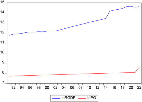
Figure 2 indicates that population growth and economic growth show a constant trend, upward trend, and decline from 1992 to 2022. However, economic growth is more cyclical relative to population growth, since population growth shows an almost constant increasing trend that of economic growth. Therefore, their relationship is far apart, which is why it is still debatable.

Figure 2. Trend between population and Economic growth rate in Ethiopia from the period 1991–2022.

Source: Computation from Eviews 10 output based on UN projection and WB, 2023, and NBE report, 2021/2022.

4.3. Causality test/using block exogeneity test

A causality test was conducted to identify the presence and direction of the causality. To identify whether a variable is weakly exogenous or endogenous, block exogeneity must be employed. That is:

• H₀ = variables are weakly exogenous

• H₁ = variables are endogenous; if the p-value is less than 5%, the null hypothesis is rejected against the alternative.

In Table 4, RGDP is weakly exogenous in explaining population growth. In addition, population growth is also weakly exogenous to explain economic growth because a p-value greater than 5% causes a failure to reject the null hypothesis. Hence, both population and economic growth are exogenous in the model and this result is consistent with (Dawson & Tiffin, 1998).

Table 4. Causality test.

Granger Causality/Block Erogeneity Wald Tests Dependent variable: LNRGDP
Excluded	Chi-sq	Prob
LNPG	1.429546	0.2318
LN_MS_P_	0.396729	0.5288
LN_ED_GDP_	0.050897	0.8215
INF	0.084409	0.7714
Granger Causality/Block Erogeneity Wald Tests Dependent variable: LNPG
Excluded	Chi-sq	Prob.
LNRGDP	0.387998	0.5334
LN_MS_P_	4.149010	0.0417
LN_ED_GDP_	0.292413	0.5887
INF	0.316610	0.5737

4.4. Cointegration and VECM

These models are employed to show the long and short term relationships between population and economic growth. All variables in the study are stationary at the first difference but not at level, indicating that they have a long-run connection and are co-integrated. As a result, we can estimate the variables’ long-run equilibrium connection in the Johansen test and then choose the VECM. As the variables are integrated of order one and co-integrated, also has an equilibrium error correction representation that is observationally equivalent, but which facilitates estimation and hypothesis testing, as all terms are stationary. In addition, VECM is a method for balancing an economic variable’s short and long-term behavior. It is a specific instance of VAR for variables whose difference is stationary (I(1)). The VECM could also consider any co-integrating relationship (Ayanaw, 2020).

The VECM is crucial for determining the gap between short term and long-term adjustments. Thus, the amount of short-term disruption produced must be quantified. The coefficients, which are predicted to be in the range of 0 to 1, show the proportion of the variable’s disequilibrium throughout a certain period if the coefficients are statistically significant and negative, they will be adjusted in the next period. If the coefficients are 1 and 0, the short run will be corrected by 100% annually, indicating that it will take a long time to close the gap between the short and long-run equilibriums, which can be described by the error correction model (-0.089021), which is less than one and negative and will be corrected by 8.9021 per-cent of each year.

The cointegration test demonstrated that there was one cointegrating vector in the model. In addition, the VECM estimation allows the long-run error correction model for the single co-integrated equation to be presented either in terms of function or outcome. Therefore, based on Tables 5 and 6, the result shows that the short run and long run dynamics of the VECM and long-run error correction model are as follows: $${\mathrm{ }\mathit{\text{ECM}}}_{1,t-1}={\mathrm{\text{ln}}\hspace{0.17em}{\mathit{\text{RGDP}}}_{t-1}-102.4658+13.89011l\mathit{\text{nPG}}}_{t-1}-3.222915\mathit{\text{ln}}{\left(\frac{\mathit{\text{Ms}}}{P}\right)}_{t-1}+0.862275\mathit{\text{ln}}{\left(\frac{\mathit{\text{ED}}}{\mathit{\text{GDP}}}\right)}_{t-1}+0.036057{\mathit{\text{Inf}}}_{t-1}$$

Table 5. Long-run relationship of cointegrated vectors.

Cointegrating Eq:	CointEq1
LNRGDP(-1)	1.000000
LNPG(-1)	13.89011
	(3.28872)
	[ 4.22357]
LN_MS_P_(-1)	−3.222915
	(0.44704)
	[-7.20944]
LN_ED_GDP_(-1)	0.862275
	(0.14076)
	[ 6.12577]
INF(-1)	0.036057
	(0.01099)
	[ 3.28104]
C	−102.4658

Table 6. Short run dynamics of VECM.

Error Correction:	D(LNRGDP)	D(LNPG)	D(LN_MS_P_)	D(LN_ED_GDP_)	D(INF)
CointEq1	−0.089021	−0.002761	0.117133	−0.256570	−18.06627
	(0.10985)	(0.00167)	(0.07406)	(0.24725)	(4.17256)
	[−2.08104]	[−1.65174]	[ 1.58150]	[−1.03771]	[−4.32978]
D(LNRGDP(−1))	0.103326	0.003829	0.063048	0.041039	11.98216
	(0.23535)	(0.00358)	(0.15868)	(0.52973)	(8.93975)
	[ 0.43903]	[ 1.06930]	[ 0.39732]	[ 0.07747]	[ 1.34032]
D(LNPG(−1))	−3.361901	1.712302	−36.51908	5.175233	2839.242
	(36.0109)	(0.54792)	(24.2802)	(81.0538)	(1367.87)
	[−0.09336]	[ 3.12511]	[−1.50407]	[ 0.06385]	[ 2.07567]
D(LN_MS_P_(−1))	−0.212125	−0.009688	−0.069729	−1.012102	36.14779
	(0.35858)	(0.00546)	(0.24177)	(0.80709)	(13.6205)
	[−0.59157]	[−1.77577]	[−0.28841]	[−1.25401]	[ 2.65392]
D(LN_ED_GDP_(−1))	0.065167	0.002381	−0.018263	0.399477	7.333830
	(0.10975)	(0.00167)	(0.07400)	(0.24702)	(4.16870)
	[ 0.59380]	[ 1.42572]	[−0.24681]	[ 1.61720]	[ 1.75926]
D(INF(−1))	0.000844	1.75E−05	−0.006899	−0.004487	−0.078999
	(0.00277)	(4.2E−05)	(0.00187)	(0.00624)	(0.10531)
	[ 0.30430]	[ 0.41439]	[−3.69055]	[−0.71905]	[−0.75017]
C	0.142857	−0.008922	0.537316	−0.007428	−39.62761
	(0.44927)	(0.00684)	(0.30292)	(1.01123)	(17.0656)
	[ 0.31797]	[−1.30512]	[ 1.77378]	[−0.00735]	[−2.32207]

In the long run, the errors are assumed to be zero and the result can be written as $${\mathrm{\text{ln}}\hspace{0.17em}{\mathit{\text{RGDP}}}_{t-1}=102.4658-13.89011l\mathit{\text{nPG}}}_{t-1}+3.222915\mathit{\text{ln}}{\left(\frac{\mathit{\text{Ms}}}{P}\right)}_{t-1}-0.862275\mathit{\text{ln}}{\left(\frac{\mathit{\text{ED}}}{\mathit{\text{GDP}}}\right)}_{t-1}-0.036057{\mathit{\text{Inf}}}_{t-1}$$

As can be seen from Tables 5 and 6, inflation positively impacts economic growth in the short term but negatively in the long term. In addition, population growth and the external debt-to-GDP ratio positively affect economic growth in the short term. Real money supply positively affects economic growth, and the external debts to GDP ratio and inflation rate have a negative and significant impact on real GDP in the long run. Therefore, the above estimation results indicate that population growth has a negative and significant impact on real gross domestic product in the long run. As population growth increases by a unit, economic growth decreases by 13.89%. This finding is consistent with (Abayneh & Belay, 2015; Adisu, 2019; and Malthus theory, 1798; Odusina et al., 2017; Ukpolo, 2002; Yao et al., 2013). Our results differ from others who find that population growth harms economic growth in the short term but has positive effects in the long term, contrary to our findings. Furthermore, our findings focus on the dual effect of population growth on economic growth rather than the single effect. Moreover, the external debt-to-GDP ratio and inflation rate have negative and significant impacts on real GDP in the long run. On the other hand, in the long run, real money supply positively affects economic growth by 0.0329%, which is consistent with many monetarist views. This result is consistent with (Chaitip et al., 2015). In addition, the external debt-to-GDP ratio has a negative and significant impact on real GDP in the long run. This finding is also similar to those (Were, 2001 in Kenya, Teklu et al., 2014 in Ethiopia, and Kharusi & Ada, 2018) in Oman’s economy. Finally, the inflation rate has a negative and significant impact on real GDP in the long run. This is also consistent with (Luppu, 2009 in Romania; and Khan & Naushad, 2020 in World economy).

In addition, different diagnostic tests were carried out. The test shows that there is no heteroscedasticity problem and no serial correlation problem because the probability (p) is greater than 5%. Therefore, the model was reliable and adequate.

5. Conclusion and recommendations

This study empirically investigates the dynamic effects of population and economic growth in Ethiopia. The analysis was performed using the Vector Error Correction Model (VECM) and was estimated using annual data for the period from 1991 to 2022. The study finds² that the short run effect of population growth has a positive effect on economic growth. This finding is in line with (Boserup, 1965; Easterlin, 1968; Kremer, 1993), however, it has a negative effect in the long run. This shows that population growth has a greater short term impact on economic growth than it does in the long term. In other words, the costs of high population growth vary from nation to nation. These variations go beyond the differences in available natural resources. A lack of natural resources does matter in nations where agriculture is very important, and poor education and low income contribute to drivers of fast population growth, making it more difficult to make the necessary changes, which have an adverse long-term effect on growth. In addition, both the external debt-to-GDP ratio and inflation have a positive and statistically significant impact on economic growth. More specifically, the ratio of external debt to GDP and inflation has beneficial short run effects on economic growth but has a negative, statistically significant long-run effect on growth. Based on the findings of the study, we highly recommend taking into account the implications of population growth on economic growth, both in the short term and the long term. The research indicates that in the short run, population growth has a positive impact on economic growth, supporting the findings of Kremer (1993), Easterlin (1968), and Boserup (1965). However, in the long run, it demonstrates a negative effect. Consequently, uncontrolled population growth exerts a detrimental influence on the economy, emphasizing the importance of implementing policies that strike a balance between economic growth and population growth.

In light of this, we suggest that the government of the country formulates a strategic plan to review family planning policies and promote liberal education. These measures will help to preserve the positive effects of population size on economic growth and contribute to growth through research and development. This recommendation holds significance as it underscores the need to carefully manage population growth in order to achieve sustainable economic growth. While high population growth might provide an initial boost to economic growth, it can lead to challenges in the long term. These challenges are not exclusively determined by the availability of natural resources; they also encompass factors such as education, income levels, and the capacity to implement necessary changes.

Moreover, the government should adopt measures aimed at improving the real money supply to stimulate economic growth. By doing so, investment will increase, leading to a rise in the demand for goods and services and ultimately resulting in output growth. Consequently, it is essential to recognize that addressing one aspect of macroeconomic instability alone may not be sufficient to foster economic growth. A comprehensive approach is required. Further investigation is also warranted, as population growth and economic growth have dual effects on the economy, both in the short term and the long term, despite the absence of a causal relationship between them. This finding aligns with the Neutralist Argument. Policymakers should, therefore, assess the specific context of their nation and carefully consider the potential costs associated with high population growth. This understanding will facilitate the identification of appropriate strategies to mitigate the adverse long term effects of population growth and promote sustainable economic growth.

6. Limitations and further recommendations

This study faces challenges due to the limited availability of data from a single source, making it difficult to obtain consistent figures for the same variables within the same source. In addition, the study is confined to analysing the dynamics of population and economic growth solely based on time series data. Thus, further studies are recommended to examine the dynamics of population and economic growth using panel data. In addition, this study used a VECM, which is widely used to show the dynamic effects of macroeconomic variables in econometric analysis, but this model has its drawbacks such as we can only conduct for series with stationarity differences of (I) 1, there is substantial disagreement over how the lag length should be determined, and degrees of freedom may be affected if a model with many explanatory variables of varying signs is ultimately established. Hence, further studies are recommended to use alternative methods and different models at a time.

Authors’ contributions

The authors contributed to the study of the dynamic effects of population and economic growth. Material and methods preparation, data collection, and analysis were performed by Tesfahun Ayanaw Alemu and Mesele Belay Zegeye. The introduction and literature part of the manuscript was written by Tesfahun Ayanaw Alemu. The method and analysis were drafted by Mesele Belay Zegeye. Finally, the manuscript is revised by Tesfahun Ayanaw Alemu. Hence, all authors have contributed to the manuscript of the research, to the analysis of the results, and to the writing of the manuscript.

Disclosure statement

No conflict of interest received by the author(s).

Data availability statement

Data will be made available on request.

Additional information

Funding

No funding was received.

Notes on contributors

Tesfahun Ayanaw Alemu

Tesfahun Ayanaw Alemu, Lecturer, Department of Economics, Woldia University, Woldia, Ethiopia; Tesfahun Ayanaw Alemu, the author of this article,has an MSc holder in Development Economics from Bahir Dar University. Currently, I am working for Woldia University as a Lecturer. I am interested in conducting a study on economic growth, development, and macroeconomic issues.

Mesele Belay Zegeye

Mesele Belay Zegeye, Assistant professor, Department of Economics, Woldia University, Woldia, Ethiopia; Mesele Belay Zegeye has an MSc in Development Economics from Debre Berhan University and he is serving Woldia University as an Assistant professor in Economics.

Notes

1 Variables are selected based on Mankiw (1998), Barro (1995), Chaitip et al. (2015), Teklu et al. (2014), Khan & Naushad (2020), Malthus (1798) and Boserup (1965).

2 However, the findings of this study are consistent with other several studies on the dynamics of population and economic growth, our study does not claim that these results apply to all other countries. The result of the study depends only on the economic structure and the interaction between the different economic actors in a given country. Hence, the estimated results of this study should be interpreted carefully, while considering them country-specific.

References

- Abayneh, A. W., & Belay, S. (2015). The environmental implication of population dynamics in Ethiopia. International Journal of Research in Agricultural Sciences, 2, 1–17.
- Abbasi, K. R., Shahbaz, M., Jiao, Z., & Tufail, M. (2021). How do energy consumption, industrial growth, urbanization, and CO2 emissions affect economic growth in Pakistan? A novel dynamic ARDL simulations approach. Energy, 221, 119793. https://doi.org/10.1016/j.energy.2021.119793
- Adisu, A. D. (2019). The nexus between population and economic growth in Ethiopia: An empirical inquiry. International Journal of Business and Economic Sciences Applied Research (IJBESAR), 12(3), 43–50.
- Akintunde, T. S., & Oladeji, P. A. O. S. I. (2013). Population dynamics and economic growth in Sub-Saharan Africa. Population, 4(13), 148–157.
- Anudjo, E. Y. (2015). The population growth-economic growth nexus: New evidence from Ghana [Doctoral dissertation]. University of Ghana.
- Assefa, H. (1994). Population dynamics and their underlying implications for development in Ethiopia [Paper presentation]. MoPED, Integrating Population and Development Planning, Addis Ababa. May.
- Asteriou, D., & Hall, S. G. (2011). Applied econometrics. Palgrave Macmillan.
- Ayanaw, T. (2020). The nexus between devaluation, external debt, and economic growth in Ethiopia (Thesis). http://ir.bdu.edu.et/bitstream/handle/123456789/11421/tesfahun%20final%20paper.pdf?isAllowed=y&sequence=1
- Barro, R. J. (1995). Inflation and economic growth. The NBER working paper 5326, Cambridge, MA, 1–22.
- Bloom, D. E., & Canning, D. (2001). Economic growth and the demographic transition, Working Paper 8685. http://www.nber.org/papers/w8685
- Boserup, E. (1965). The conditions of agricultural growth: The economics of agrarian change under population pressure. Aldine.
- Calderón, C., & Fuentes, J. R. (2013). Government debt and economic growth. (No.IDB-WP-424). IDB Working Paper Series.
- Chaitip, P., Chokethaworn, K., Chaiboonsri, C., & Khounkhalax, M. (2015). Money supply influencing economic growth-wide phenomena of AEC open region. Procedia Economics and Finance, 24, 108–115. https://doi.org/10.1016/S2212-5671(15)00626-7
- Clarke, C. (1967). Land use and population growth. UK: Palgrave Macmillan. https://doi.org/10.1016/S2212-5671(15)00626-7
- Coale, A. J., & Hoover, E. M. (1958). Population growth and economic development. Princeton University Press.
- Dawson, P. J., & Tiffin, R. (1998). Is there a long‐run relationship between population growth and living standards? The case of India. Análisis Económico, Núm. 77, vol. XXXI.
- Dennis, A., & Robert, C. (2008). Population and development. In International handbook of development economics (pp. 316–327). Edward Elgar.
- Dickey, D. A., & Fuller, W. A. (1979). Distribution of the estimators for autoregressive time series with a unit root. Journal of the American Statistical Association, 74(366), 427–431. https://doi.org/10.2307/2286348
- Dyson, T. (2010). Population and development: The demographic transition. Zed Books.
- Easterlin, R. A. (1968). Population, labor force, and long swings in economic growth. National Bureau of Economic Research.
- Enders, W. (1995). Applied econometric time series (1 ed.). Ed. John Willey & Sons.
- Engel, R. F., & Granger, C. W. J. (1987). Cointegration: Representation, estimation, and testing. Journal of Econometrics, 35, 199–235.
- Granger, C. W., & Newbold, P. (1974). Spurious regressions in econometrics. Journal of Econometrics, 2(2), 111–120. https://doi.org/10.1016/0304-4076(74)90034-7
- Harris, R., & Sollis, R. (2003). Applied time series modeling and forecasting. Wiley.
- Hendry, D., & Juselius, K. (2000). Explaining cointegration analysis: Part II. The Energy Journal, 21(1), 1–42. https://doi.org/10.5547/ISSN0195-6574-EJ-Vol21-No1-1
- IMF. (2020). World economic outlook update. June, 2020.
- Johansen, S. (1988). Statistical analysis of cointegration vectors. Journal of Economic Dynamics and Control, 12(2-3), 231–254. https://doi.org/10.1016/0165-1889(88)90041-3
- Kalemli-Ozcan, S. (2002). Does the mortality decline promote economic growth? Journal of Economic Growth, 7(4), 411–439. https://doi.org/10.1023/A:1020831902045
- Khan, I., Hou, F., Le, H. P., & Ali, S. A. (2021). Do natural resources, urbanization, and value-adding manufacturing affect environmental quality? Evidence from the top ten manufacturing countries. Resources Policy, 72, 102109. https://doi.org/10.1016/j.resourpol.2021.102109
- Khan, I., Zakari, A., Ahmad, M., Irfan, M., & Hou, F. (2022). Linking energy transitions, energy consumption, and environmental sustainability in OECD countries. Gondwana Research, 103, 445–457. https://doi.org/10.1016/j.gr.2021.10.026
- Khan, N., & Naushad, M. (2020). Inflation relationship with the economic growth of the world economy. Available at SSRN 3542729.
- Kharusi, S. A., & Ada, M. S. (2018). External debt and economic growth: The case of an emerging economy. Journal of Economic Integration, 33(1), 1141–1157. https://doi.org/10.11130/jei.2018.33.1.1141
- Kidane, A. (2020). The Impact of population growth on economic growth: Evidence from Ethiopia using ARDL approach. Journal of Economics and Sustainable Development, 11(3), 19–33.
- Kremer, M. (1993). Population growth and technological change: One million BC to 1990. The Quarterly Journal of Economics, 108(3), 681–716. https://doi.org/10.2307/2118405
- Kuo, C. Y. (2016). Does the vector error correction model perform better than others in forecasting stock price? An application of residual income valuation theory. Economic Modelling, 52, 772–789. https://doi.org/10.1016/j.econmod.2015.10.016
- Linden, E. (2017). Remember the population bomb? It’s still ticking. New York Times: Sunday Review, 4.
- Luppu, D. V. (2009). The correlation between inflation and economic growth in Romania. Luccrari Stiintifice, 53, 359–363.
- Malthus, T. R. (1798). An essay on the principles of population. Cambridge University Press.
- Mamingi, N., & Perch, J. (2013). Population growth and economic growth/development: An empirical investigation for Barbados. Population, 4(4), 93–105.
- Mankiw, N. G. (1998). Teaching the principles of economics. Eastern Economic Journal, 24(4), 519–524.
- Mohsen, A. S., & Chua, S. Y. (2015). Effects of trade openness, investment and population on the economic growth: A case study of Syria. Hyperion Economic Journal, Year, 3(2), 3.
- National Bank of Ethiopia. (2021/2022). 10th edition.
- Odusina, E. K., Kupoluyi, J. A., & Gbadebo, B. M. (2017). Implications of a rapidly growing Nigerian population. EBSU Journal of Social Sciences and Humanities, 1(2).
- Ogundipe, A., Ojeaga, P., & Ogundipe, O. (2013). Estimating the long-run effects of exchange rate devaluation on the trade balance of Nigeria. European Scientific Journal, 9(25), 233–249.
- Okunolа, A. M., Nathaniel, S. P., & Festus, V. B. (2018). Revisiting population growth and food production nexus in Nigeria: an ARDL approach to cointegration. Agricultural and Resource Economics: International Scientific E-Journal, 4(4), 41–51. https://doi.org/10.51599/are.2018.04.04.04
- Sadiq, M., Hassan, S. T., Khan, I., & Rahman, M. M. (2023). Policy uncertainty, renewable energy, corruption, and CO2 emissions nexus in BRICS-1 countries: a panel CS-ARDL approach. Environment, Development and Sustainability. https://doi.org/10.1007/s10668-023-03546-w
- Sibe, J. P., Chiatchoua, C., & Megne, M. N. (2016). The long run relationship between population growth and economic growth: a panel data analysis of 30 of the most populated countries of the world. Análisis Económico, 31(77), 205–218.
- Simon, J. (1977). The economics of population growth. Princeton University Press.
- Sims, C. A. (1980). Macroeconomics and Reality. Econometrica, 48(1), 1–48. https://doi.org/10.2307/1912017
- Solow, R. M. (1956). A contribution to the theory of economic growth. The Quarterly Journal of Economics, 70(1), 65–94. https://doi.org/10.2307/1884513
- Stock, J. H., & Watson, M. W. (2007). Introduction to econometrics (2nd ed.). Pearson Education.
- Tartiyus, E. H., Dauda, T. M., & Peter, A. (2015). Impact of population growth on economic growth in Nigeria. IOSR Journal of Humanities and Social Science (IOSRJHSS), 20(4), 115–123.
- Tasew, T. (2011). Foreign aid and economic growth in Ethiopia. https://mpra.ub.uni-muenchen.de/33953/1/MPRA_paper_33953.pdf
- Teklu, K., Mishra, D. K., & Melesse, A. (2014). Public external debt, capital formation and economic growth in Ethiopia. Journal of Economics and Sustainable Development, 5, 58–70.
- Terefe, D. (2018). Economy and population in Ethiopia: a search for relations. Journal of Economic & Social Development, 14(2).
- Thuku, G. K., Gachanja, P. M., & Obere, A. (2013). The impact of population change on economic growth in Kenya. International Journal of Economics and Management Sciences, 2(6), 43–60.
- Udemba, E. N. (2020). Ecological implication of offshored economic activities in Turkey: foreign direct investment perspective. Environmental Science and Pollution Research International, 27(30), 38015–38028. https://doi.org/10.1007/s11356-020-09629-9
- Ukpolo, V. (2002). Population growth and economic growth in Africa. Journal of Developing Societies, 18(4), 315–329. https://doi.org/10.1177/0169796X0201800402
- Wang, Q., Wang, X., & Li, R. (2022). Does urbanization redefine the environmental Kuznets curve? An empirical analysis of 134 Countries. Sustainable Cities and Society, 76, 103382. https://doi.org/10.1016/j.scs.2021.103382
- Wang, Q., Zhang, F., & Li, R. (2023). Free trade and carbon emissions revisited: The asymmetric impacts of trade diversification and trade openness. Sustainable Development, 32(1), 876–901. https://doi.org/10.1002/sd.2703
- Were, M. (2001). The impact of external debt on economic growth in Kenya: An empirical assessment. (No. 2001/116). WIDER Discussion Papers//World Institute for Development Economics (UNU-WIDER).
- World Bank open data. (2023). World Bank open data. https://data.worldbank.org/
- Wuletaw, M. (2018). The link between agricultural production and population dynamics in Ethiopia: A review. Advances in Plants & Agriculture Research, 8(4), 348–353.
- Yahaya, N. S. (2019). Population growth and environmental degradation in Nigeria. 826651216.
- Yang, X., & Khan, I. (2022). Dynamics among economic growth, urbanization, and environmental sustainability in IEA countries: the role of industry value-added. Environmental Science and Pollution Research International, 29(3), 4116–4127. https://doi.org/10.1007/s11356-021-16000-z
- Yao, W., Kinugasa, T., & Hamori, S. (2013). An empirical analysis of the relationship between economic development and population growth in China. Applied Economics, 45(33), 4651–4661. https://doi.org/10.1080/00036846.2013.795284
- Yigermal, M. (2018). Devaluation, balance of payment and output dynamics in developing countries (the case of Ethiopia). Addis Ababa University.
- Zahoor, Z., Khan, I., & Hou, F. (2022). Clean energy investment and financial development as determinants of environment and sustainable economic growth: evidence from China. Environmental Science and Pollution Research, 29(11), 16006–16016. https://doi.org/10.1007/s11356-021-16832-9
- Zakari, A., Khan, I., & Alvarado, R. (2023). The impact of environmental technology innovation and energy credit rebate on carbon emissions: A comparative analysis. Journal of International Development, 35(8), 2609–2625. https://doi.org/10.1002/jid.3788