The influence of household size on socioeconomic conditions of rural farm households in Damot Woyde District, Wolaita Zone, Southern Ethiopia

Abstract

There is little debate about the relationship between rising fertility and declining income. Rapid population growth can have serious implications for people’s standard of living—their incomes, savings, health, education, and general well-being. Thus, the objective of this study is to analyze the impacts of household sizes on rural farm households’ savings, consumption spending, and financial capacity to cover the expenses of children’s education and the health of household members. 346 rural farm household heads took part in the study, which used a multistage sample technique. Along with the survey results, six focus group discussions, 27 key informant interviews, and personal observations were done. The outcomes showed that the savings-to-income ratios of rural households decreased with increasing household size, whereas consumption-to-income ratios increased due to a portion of the income that was not saved being spent on supporting the consumption demands of the additional household member. The MANOVA post hoc analysis also revealed that the large household size group’s average yearly savings were significantly lower than the small household size group, whereas consumption expenses grew with increasing household size. Furthermore, ordinal logistic regressions show that increasing household size without increasing income diminishes rural farm households’ existing financial capacity to afford the expenditures of their children’s education and healthcare for household members. Thus, it is preferable to advocate that rural households have access to quality reproductive health-care services, like safe and effective family planning alternatives, and that households strive to diversify their income sources to promote savings.

Keywords:

• Household size
• savings
• consumption costs
• rural households
• Damot Woyde

Reviewing Editor:

• Michael Hardman, University of Salford, Salford, UK

Subjects:

• Rural Development
• Development Policy
• Economics and Development
• Health & Development
• Sustainable Development
• Human Geography
• Sociology & Social Policy

1. Introduction

Globally, rapid population growth is causing anxiety and posing a threat to countries’ economies. Since the mid-twentieth century, the population of the world has more than tripled, hitting almost 8 billion people in 2022, and UN forecasts indicate that the global population might reach nearly 11 billion by about 2100 (Wilmoth et al., 2022). Even if fertility rates continue to drop, Sub-Saharan African nations (including Ethiopia) might account for more than half of global population growth between 2019 and 2050 (United Nations DESA Population Division, 2019). Rapid population growth could aggravate the difficulty of guaranteeing sustainable and inclusive future development. Attaining the sustainable development goals, especially those concerning health, education, and gender equality, can help slow down the global population increase (Wilmoth et al., 2022).

The relationship between population change and socioeconomic outcomes has been debated by economists, demographers, and other social scientists. There are three positions that have emerged: one that claims that population growth benefits a nation’s economy by stimulating economic growth and development, and another that bases its theory on Robert Malthus’ findings, which claim that population growth is detrimental to a nation’s economy due to a variety of problems caused by the growth. The third school of thought contends that population growth has no effect on economic growth (Chikaodilli et al., 2020; Obere et al., 2013). Despite these arguments, a general agreement has emerged over time that when fertility or household size grows, income tends to fall. There is little debate about the relationship between rising fertility and declining income. In general, there has been a consistently high association between dropping birth rates and national income growth, as well as between household income and fertility. Economists and demographers generally believe that a lack of key components for improving living standards, such as urbanization, industrialization, improved job opportunities, higher educational attainment, and better health, all contribute to low socioeconomic conditions (Sinding, 2008). Rapid population growth can have serious implications for people’s standard of living—their incomes, savings, health, education, and general well-being (Todaro & Smith, 2015).

Although it is not the cause of economic stagnation, evidence suggests that rapid increase in population reduces per capita income growth in most developing nations, particularly those that are already poor, reliant on agriculture, and facing land and natural resource constraints (Todaro & Smith, 2012). It is widely accepted that large household sizes and low finances limit parents’ ability to educate all of their children. A rapid rise in the population causes educational spending to be spread more thinly at the national level, sacrificing quality for the sake of quantity. This, in turn, feeds back on economic growth since a high population increase depletes the supply of human capital (Blaabæk et al., 2017; Rizk et al., 2019; Shen, 2017; Todaro & Smith, 2015). High fertility impairs the health of mothers and children by increasing pregnancy risks, and closely spaced deliveries have been indicated to negatively affect birth weight and boost child death rates (Kitole et al., 2022; Todaro & Smith, 2012; Van Minh et al., 2013). In general, large household sizes lower income and savings while increasing consumption expenditure in impoverished countries, reducing their ability to invest in human capital such as education and the health of household members (Todaro & Smith, 2015).

Ethiopia is the world’s 12th and Africa’s second-most populous country, according to the WHO, with a population of 102 million and a growth rate of 2.6% in 2020 (WHO, 2022). During the same year, the Ethiopian economy faced a number of issues that jeopardized the country’s macroeconomic stability, including high inflation, a lack of foreign exchange, a large debt burden, and low utilization of internal resources (UNICEF Ethiopia, 2022). According to UNICEF report, Ethiopia’s inflation rate peaked at 37.2% in June 2022, ranking third in Africa and eighth in the world. Food price inflation rose significantly from 23.9% in May 2021 to 42% in October 2022. Total domestic savings, on the other hand, fell from 24.3% in 2017/18 to 15.3% in 2021/22, while total consumption spending climbed from 75.7% in 2017/18 to 84.7% in 2021/22 (National Bank of Ethiopia, 2022).

Any country’s economic development is dependent on its people’s saving capacity and spending habits. The dependent family or household size is an important determinant in determining an individual’s saving and subsequent spending behavior (Kiran & Dhawan, 2015). The empirical findings of the majority of studies suggest that as the size of the household increases, income is diverted away from savings, lowering the individual’s saving income ratio (Lugauer et al., 2017; Lidi et al., 2017). Consumption expenditure, in contrast, is considered a positive function of household size, and every increase in family size imposes additional pressure on the household’s current income levels, resulting in a diversion of resources towards consumption (Kiran & Dhawan, 2015).

Wolaita Zone, where the current study district is located, has long been connected with a large population and a subsistence economy. Wolaita Zone has one of the highest population densities in the country, with an average density of 497 persons per square kilometer (Central Statistical Agency (CSA), 2020). The area’s population is rising at a rate of more than 3% per year (CSA, 2016), resulting in a number of socioeconomic constraints. Previous population-related studies, for instance (Babiso et al., 2020; Dana, 2008, 2015; Dana et al., 2020), conducted in the Wolaita zone in general and the study district, Damot Woyde in particular, looked at rapid rural population growth and its drivers, population pressure and food security, and population growth and environmental alterations. However, none of the associated research addressed the demographic pressures caused by large household sizes on household savings, consumption spending, and human capital investments. Thus, the objective of this study is to analyze the impacts of household sizes on rural farm households’ savings, consumption spending, and financial capacity to cover the expenses of children’s education and the health of household members, as well as to fill gaps in prior studies.

2. Materials and methods

2.1. Description of the study area

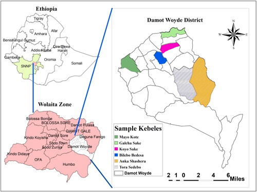
This study was conducted in the Damot Woyde district, Wolaita zone, southern Ethiopia. The study district is located between 6° 40′56″ and 6° 59′30″ N latitudes and 37° 52′20″ and 38° 04′35″ E longitudes (Figure 1). Bedessa, the administrative center of the district, is located 335 kilometers south of Addis Ababa and 26 kilometers east of Sodo, the capital of the Wolaita Zone. The district now contains 24 kebeles (the smallest administrative level in Ethiopia). The district covers 352 square kilometers with a population of 121,478 (CSA, 2020). The study district is characterized by two agro-climatic zones (ACZs): Woina Dega (Midland, 60%) and Kolla (Lowland, 40%). Woina Dega is 1600–2100 m above sea level, while Kolla is 1000–1600 m (Bergene, 2014). The study district has two primary rainy seasons: (Meher) June-October and (Belg) March-May, while rainfall amounts and intensity vary throughout the year. In the study area, small-scale farming is the main source of livelihood, with some non-farms and off-farms. Enset (Ensete ventricosum), cereals, and root crops are the principal crops grown in the district (Bergene, 2014).

Figure 1. Location map of the study area.

2.2. Research design and sampling techniques

A cross-sectional household survey and a quantitative dominant mixed research design were utilized in this study. Convergent mixed techniques allow for the collection of qualitative and quantitative data simultaneously (Creswell & Creswell, 2018). A multistage sampling strategy was used for this study. The first stage was to purposely select the study district due to the lack of existing research on the effects of population pressure on farm households’ savings, consumption expenses, and financial capacity to invest human capital. The study district was then stratified into two ACZs to encompass both ACZs of the district in the second step. In the third step, four kebeles were picked at random from Woina Dega and two from Kolla based on their ACZ proportionality. Finally, 346 sample households were chosen at random in the fourth stage using the Kothari (2004) sample size determination formula: $$\mathit{n}=\frac{{\mathit{Z}}^2\mathrm{*}\mathit{p}\mathrm{*}\mathit{q}\mathrm{*}\mathit{N}}{{\mathit{e}}^2\mathrm{*}\left(\mathit{N}-1\right)+{\mathit{Z}}^2\mathrm{*}\mathit{p}\mathrm{*}\mathit{q}}$$ where, z = 1.96 (95% confidence interval); p = sample proportion, 0.5; q = 1-p; e = error margin = 0.05 (5%); N = total number of households (sampling frame) =3327.

2.3. Data sources and Methods of collection

Primary and secondary data sources were used to achieve the specified objectives. The primary data were collected by a household questionnaire survey that was conducted from March to May 2022. Additional data were harvested from 27 key informants (KIIs), six focus group discussions (FGDs) with 8 to 12 members at each session, and field observations to supplement and corroborate the quantitative data. Secondary data was gathered using important published and unpublished materials, such as books, journal articles, websites, papers, and government reports.

2.4. Methods of data analysis

In this study, the researcher used both descriptive and econometric analysis to examine the impact of household size on rural farm households’ saving, consumption expenditure, and the financial ability to cover children’s educational and household members’ health costs. The single-factor MANOVA was used to analyze the effect of household size on annual savings and consumption expenses of rural households, and ordinal logistic regression (OLR) was used to examine the effect of household size on the households’ ability to finance education and health costs.

2.4.1. Single-factor multivariate analysis of variance (MANOVA)

MANOVA is used to investigate the multivariate effect (how the predictor variables affect the combination of response variables) and the univariate effect (how the mean scores for each response variable vary across independent variable groups) (Mayers, 2013). According to Field (2009), Single-Factor Multivariate Analysis of Variance (MANOVA) is a statistical technique to analyze the difference between the mean values of multiple dependent variables across different categories (groups) of a single independent variable. In general, MANOVA is only used when there is a low to moderate amount of correlation between the dependent variables (negative correlation up to -.40; positive correlation between .30 and .90) (Brace et al., 2016). Taking into mind the explanations for these rules, the researcher employed the MANOVA approach to determine if the mean yearly savings and mean yearly consumption costs of households differ significantly across various household size groups.

The outcome and factor variables used in the MANOVA procedure are shown in Table 1, which shows the household size of rural farm households is categorized into three household size groups, with an average household size of 6.64 members. Based on this average household members as a mid-point, the researcher grouped the household sizes as small (five and below members), medium (six to seven members) and large (eight and above members). The modest negative Pearson correlation value (−0.031) among savings and consumption costs confirms that the two outcome variables are conceptually linked and correlated at a lower level (Table 1). This indicates that the single factor MANOVA method was the best statistical tool for analyzing and comparing the two response variables (average yearly savings and average consumption expenses) simultaneously across multiple levels of one independent variable (3 various household groups).

Table 1. Description of the variables employed in the MANOVA analysis.

Outcome Variables	Independent variable (household size)	Sample size
A.Annual estimated savings (ETB*)	Small household size	74
B.Annual estimated consumption expense (ETB)	Medium household size	195
	Large household size	77
	Total = 3 groups	346
Pearson correlation between savings and consumption expenditure = −0.031

*ETB: The national currency of Ethiopia.

2.4.2. Ordinal logistic regression

The researcher used OLR to examine the effect of household size on some socioeconomic conditions (financial ability to cover children’s educational expenses and health costs of household members) in rural farm households. It has multiple OLR methods that take the ordinal results into consideration. The logits in these multiple ordinal regression methods are created in various ways. For instance, the proportional odds model (POM) (regarded as cumulative higher category(s) versus cumulative remaining lower category(s)); the continuation ratio model (CRM) (regarded as cumulative higher category(s) versus just lower category alone); and the adjacent category model (ACM) (within any two successive categories) (Lelisho et al., 2022; Singh et al., 2020). Thus, every type of logit has its own set of strengthens and limitations; the models can be used as needed. To be more precise, both CRM and ACM do not depend on the entire data set (Lelisho et al., 2022). The POM was used in the current study because it provides a more rational and intelligible analysis of socioeconomic conditions (Singh et al., 2020).

The assumptions of POM ensure the odds ratios (OR) are the same across every group. If the log OR of all the threshold points is identical, the proportional odds condition is fulfilled, and the POM is employed (Singh et al., 2020). POM is a frequently utilized approach that was announced as a cumulative logit model by Walker and Duncan (1967), yet later called a proportional odds model by McCullagh (1980). To run the outcome variables (rural households’ ability to cover children’s educational and household members health expenses), two independent ordinal logistic models were used. The socioeconomic conditions (Y) observed in each household are grouped into any of the three classes, i.e., poor ability to cover education and health expenses, fair ability to cover education and health expenses, and good ability to cover education and health expenses. Likewise, covariates (xi) denote the vector of covariates of dimension P (i = 1, 2, 3… P), which comprises all P explanatory factor observations. Consequently, the dependence of Y on xi can be written (Singh et al., 2020) as: (2) $$P(Y\ge \mathit{\text{yj}}x)=\frac{1}{1+\text{exp}\left(-\alpha j-x\prime i\beta \right)},j=1,2,3$$(2) or (3) $$\text{log\hspace{0.17em}}\left[\frac{P(Y\ge \mathit{\text{yj}}x)}{1-P(Y\ge \mathit{\text{yj}}x)}\right]=\alpha +x\prime i\beta ,j=1,2,3$$(3) where P(Y ≥ yj) denotes the cumulative possibility of the event (Y ≥ yj), αj are the respective intercept parameters, and β is a (P by 1) vector of regression coefficients corresponding to x_i covariates.

In OLR, a p-value of less than 0.05 was accepted as a statistically significant factor for the dependent variable. The p-value and odds ratio with a 95% confidence interval have been employed to indicate the statistical significance and strength of the relationship. During the analysis, the software assigned the estimates of the explanatory variables to the response variables. Thus, the odds ratio for this research was derived using the exponential of the given estimations from the final analysis output. The OLR model’s assumptions were tested. The model fitting information, the goodness of fit, pseudo-R², and the test of parallel lines were all utilized to check the model fit.

3. Results

3.1. Descriptive statistics

To describe the pattern of savings and consumption costs in rural households, the average annual savings, consumption expenditures, and income, as well as the savings-to-income and consumption-to-income ratios, were computed for any of the three household size groups. As indicated in Table 2, small rural farm households (5 and below members) have the largest average yearly savings (1,809.95 ETB), whereas large farm households (8 and above members) have the lowest (−2062.71 ETB) (Table 2). The negative sign of mean savings in medium and large rural household size groups shows their average annual consumption expenditure exceeding their average annual income, forcing farm households to owe. This means that rural households’ savings diminish as the number of household member increases.

Table 2. The descriptive statistics.

	Household size groups
	Small (n = 74)	Medium (n = 195)	Large (n = 77)	Total (n = 346)
Mean Income (S.D*)ETB	13595.33 (3677.87)	12644.23 (3031.07)	11362.32 (1919.04)	12562.37 (3064.93)
Mean Savings (S.D*)ETB*	1809.95 (1578.59)	−81.96 (1612.83)	−2062.71 (1116.66)	−118.13 (1976.55)
Mean Consumption (S.D*)ETB	11785.38 (2998.02)	12726.19 (2258.03)	13425.04 (1799.74)	12680.50 (2404.00)
Saving Income Ratio	0.133	−0.006	−0.181	−0.009
Consumption Income Ratio	0.867	1.006	1.181	1.009

* S.D: Standard deviation; (values in the parenthesis are Standard deviation), ETB: the Ethiopian Birr, the currency of Ethiopia.

In terms of consumption patterns, the average consumption expenditure rose from 11,785.38 ETB to 13,425.04 ETB when household sizes grew from small to large. In a similar vein, the consumption expenses to income ratio increases from 0.867 to 1.181 when the household size increases from small to large, respectively (Table 2). The primary explanation for the trend in consumption expenses can be attributed to meeting the consumption demands of extra household members. Furthermore, the mean values of both yearly savings and consumption expenditure varied significantly among three household groups. Yet, whether there was a significant variation in their mean values across different household size groups was determined using multivariate MANOVA testing.

3.2. Single-factor MANOVA results

3.2.1. Multivariate F-test and box’s test

The multivariate F-statistics Pillai’s Trace, Roy’s Largest Root, and Wilk’s Lambda are widely employed to determine if the three household size groups differ significantly on a linear combination of outcome variables, namely annual savings and consumption expenses (Mayers, 2013). When the Box test statistic is significant, Pillai’s Trace and Roy’s Largest Root can be employed (Mayers, 2013). As indicated in Table 3, the Box statistic was found to be statistically significant (p < 0.001); thus, Pillai’s Trace and Roy’s Largest Root were employed to determine if various groups of the independent variable differed significantly on a linear combination of outcome variables. Pillai’s Trace and Roy’s Largest Root significant values revealed that there were significant variations across the three household size groups on a linear combination of the two dependent variables (savings and consumption expenses) of rural households. We find a significant multivariate household sizes’ influence on the combined dependent variables of savings and consumption expenses (Pillai’s Trace value = 0.860, F = 51.68, p < 0.001; and Roy’s Largest Root value = 0.463, F = 147.50, p < 0.001). Yet, the significant effect fails to tell us much about the actual size of the difference in relation to the number of cases utilized to measure the variation. We need an effect size for that.

Table 3. Single-factor MANOVA Results.

Box’s Test	Multivariate F-Test			Levene’s test	Univariate F-test
	Pillai’s trace	Roy’s largest root	Wilk’s lambda
6.59***	51.68***	147.50***	62.30***	Savings = 5.22**	Savings = 124.35*** (0.420^b)
	0.860^a	0.463^a	0.537^a	Consumption = 17.49***	Consumption = 9.28***
					(0.151^b)

*** &. **: represent that test statistic is significant at 1% and 5% level respectively.

^a &.

^b : denotes the multivariate outcomes and Partial Eta Squared, respectively.

The effect size measures the actual amount of the change between scores without taking into account how it relates to the entire population (Mayers, 2013). It relies on the sample mean and standard deviation but does not take into account the standard error. The researcher used G*Power software to measure the effect size and statistical power outcomes of the results. The most frequently utilized way to measure effect size is Cohen’s d method, which explores effect size by examining differences relative to sample sizes and pooled standard deviation. Cohen categorized effect size as small when d < 0.25, medium when d 0.25 to 0.4, and large when d > 0.4 (Mayers, 2013). Based on this scenario, the overall MANOVA effect of Pillai’s trace (0.860) was calculated and resulted in an effect size (d) = 0.754 (very large) and a power (1 − β err prob) 0.97 (excellent).

3.2.2. Univariate outcome

Since the correlation between the dependent variables was not too high, we can proceed with univariate and post hoc testing (Mayers, 2013). When the multivariate F-test was found to be significant, the following step in the MANOVA technique was to verify whether the mean values of the individual outcome variable differed significantly between groups of the independent variable, which was evaluated using a univariate F-test. The two distinct significant univariate F-test results (124.35 and 9.28 for savings and consumption, respectively) revealed that the mean values of yearly savings and consumption expenses differed considerably among the three household size groups, as displayed in Table 3. The effect size each dependent variable calculated by G*Power software reveals that the annual savings and consumption expense were (d = 0.851) very large and (0.422) large, respectively.

3.2.3. Post hoc multiple comparisons

The researcher needed post-hoc tests to investigate the source of the significant difference because we had three groups for our independent variable. Table 4 displays the post hoc tests. The implementation of post hoc testing depends on the results of Levene’s test, which examines whether the variances of the dependent variable are equal or not across all independent variable groups. When Levene’s test fails to yield a significant result and an assumption of variance homogeneity is met, a post hoc test designed for equal variances, such as the Tukey HSD (honestly significant differences) test, is performed. When the assumption of variance homogeneity is not met, the post hoc test, which is specifically developed for use with the scenario of unequal variances, such as Games–Howell test is utilized (Mayers, 2013; Morgan et al., 2011). Because Levene’s test of variance homogeneity was revealed to be significant for both savings (5.22) and consumption expenses (17.49), the Games-Howell post hoc test, which is specifically used in instances with unequal variances, was employed for multiple comparisons.

Table 4. Post hoc comparisons results of MANOVA.

Dependent variables	Household size (I)	Household size (J)	Mean difference (I-J)	Std. error	Sig	95% confidence interval
						Lower bound	Upper bound
Annual Savings	Small HHS	Medium HHS	1891.92***	216.83	.000	1378.04	2405.79
		Large HHS	3872.67***	223.31	.000	3343.27	4402.06
	Medium HHS	Large HHS	1980.75***	171.85	.000	1574.95	2386.55
Annual consumption expenditure	Small HHS	Medium HHS	−940.82**	384.20	.042	−1854.09	−27.54
		Large HHS	−1639.66***	404.38	.000	−2599.46	−679.85
	Medium HHS	Large HHS	−698.84**	261.18	.022	−1316.26	−81.42

*** &. **: The mean difference is statistically significant at 1% and 5% level, respectively.

HHS: Household size group.

Table 4 reveals that the average annual savings of small household size groups are significantly higher than those of medium and large household size groups by 1891.92 ETB and 3872.67 ETB, respectively (p < 0.001) (Table 4). Similarly, the positive mean difference revealed that the mean yearly savings of medium household size groups were significantly larger than those of large household size groups (p < 0.001), even though both of their mean annual savings were negative, i.e., they owed at the end of the year (Table 2). The average yearly consumption expenses of rural farm households with smaller household sizes were identified to be significantly less than those of medium and large household sizes (p < 0.05 and p < 0.001, respectively), as indicated by the negative mean difference in consumption expenditure between them. Similarly, the mean yearly consumption expense of rural households with medium household size was significantly lower than that of large household size groups by 698.84 ETB (p < 0.05).

3.3. The results of ordinal logistic regression (OLR)

3.3.1. Socioeconomic conditions of the study participants

A total of 346 study participants were involved in the final analysis of OLR. The majority (81.5%) of the study participants were males. The average household size of the study participants is 6.64, with 4 and 13 minimum and maximum household members, respectively. The majority of the study participants had very little formal schooling, an average of 1.96. The estimated mean annual income of the participants was 12,562.37 ETB. The average distance to access the primary school and health center of the study participants was 2.85 and 9.46 km, respectively (Table 5).

Table 5. Variables descriptions of OLR.

Variables		Minimum	Maximum	Mean	Std. deviation
Household Size		4	13	6.64	1.51
Household Head’s Education		0	12	1.96	3.37
Annual Income		7625 ETB	25,210 ETB	12,562.37 ETB	3064.93
Distance to School (Km)		0.5	6	2.85	1.17
Distance to Health Center (Km)		2	23.9	9.46	4.88
Gender		Male = 282 (81.5%)	Female = 64 (18.5%)	Total = 346 (100%)

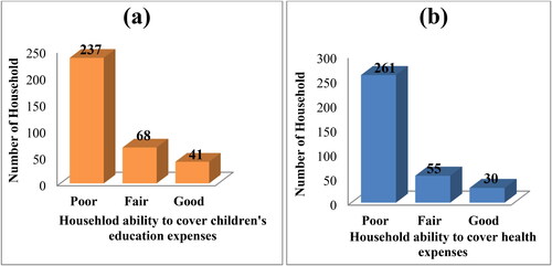
The outcome variables—the financial ability to cover the expenses of their children’s education and the health expenses of household members—of rural farm households are typically broken down into three levels (poor, fair, and good) based on participant responses to explain the three categories that a household may fall into. Two separate OLR models were employed to independently examine the children’s educational expenses and household members’ health expenses. Thus, 237 (68.5%), 68 (19.7%), and 41 (11.8%) of the 346 rural farm households studied had poor, fair, and good financial capacity to cover their children’s educational expenses, respectively (Figure 2a), and 261 (75.4%), 55 (15.9%), and 30 (8.7%) had poor, fair, and good financial capacity to cover their household members’ health costs, respectively (Figure 2b).

Figure 2. Rural household financial capacity to cover children’s education expenses (a) household members’ health expenses (b).

3.3.2. Effects of household size on households’ ability to cover children’s educational and household members’ health expenses (OLR results)

The main intention of the researcher is to examine the size of household influence on the financial capacity of rural farm households to cover their children’s educational expenses and the expenses of health for household members. However, some socioeconomic factors that were expected to have an effect on dependent variables were included as parameters to test the cumulative impact on outcome variables. Accordingly, household head’s gender, household head’s education level, income, and access to a school and health center were some of the predicted parameters that may influence rural farm households’ capacity to educate their children and protect the health of their household members. We evaluated for multicollinearity before designing the multivariate OLR model, although it is not mentioned in the current article.

The proportional odds supposition (parallel line test) is the primary supposition in OLR, which explains how the impacts of any factor variables are constant or proportional across various thresholds. If the p-value of the parallel line test is large, the proportionality condition holds. The general proportionality supposition was not broken in this investigation, as p values for OLR models 1 and 2 were 0.147 and 0.171, respectively. This result implies that the proportionality notion holds up since it has a large p value (> 0.05), which is a statistically insignificant value.

By using the multivariate POM, household size was found to be the most influential predictor of rural farm households’ financial ability to fund their children’s schooling expenses and household members’ health costs. The results from multivariable OLR (Table 6 and Table 7) showed that the households’ size was highly significant at a 1% level (p < 0.001). The expected OR (OR = 0.148, 95% CI 0.096–0.226) indicated that those households with a large household size were 0.148 times less probable to have good financial ability to cover their children’s educational expenses, keeping all other variables fixed (Table 6). In a similar vein, the expected OR (OR = 0.196, 95% CI 0.126–0.306) suggested that those with a large household size were 0.196 times less probable to have the financial ability to cover their household members’ health expenses; all other factors were held constant (Table 7).

Table 6. POM variable estimations with three-ordered categories based on household ability to cover children’s education expenses - OLR Model 1 (N = 346).

Variables	Estimate	S.E	p-value	OR	95% CI for OR
					Lower	Upper
Gender (Male)	.923	.4228	.029**	2.517	1.099	5.766
Household Head’s Education in schooling years	.071	.0460	.123	1.074	.981	1.175
Household size	−1.913	.2178	.000***	.148	.096	.226
Annual income	.000	.0000	.000***	1.000	1.000	1.000
Distance to school (km)	.107	.1342	.425	1.113	.856	1.448

Model fitting information: p-value < 0.001; Goodness-of-Fit: Pearson, p-value = 1.00, Deviance, p-value = 1.00; Pseudo R², Nagelkerke = 0.636; Parallel line test: p-value = 0.147.

Table 7. POM variable estimations with three-ordered categories based on household ability to cover health expenses of household members - OLR Model 2 (N = 346).

Variables	Estimate	S.E	p-value	OR	95% CI for OR
					Lower	Upper
Gender (male)	.634	.4721	.179	1.885	.747	4.754
Household head’s education in schooling years	.052	.0485	.288	1.053	.957	1.158
Household size	−1.628	.2270	.000***	.196	.126	.306
Annual income	.000	.0001	.000***	1.000	1.000	1.001
Distance to health center (km)	−.001	.0314	.966	.999	.939	1.062

Model fitting information: p-value < 0.001; Goodness-of-Fit: Pearson, p-value = 0.961 Deviance, p-value = 1.00; Pseudo R², Nagelkerke = 0.604; Parallel line test: p-value = 0.171.

3.3.3. Model fitting assessment

The goodness of fit check reveals that both the Pearson and deviance statistics (p = 1.000) for OLR model 1 and Pearson (p = 0.961) and deviance (p = 1.000) for OLR model 2 are large. This pointed out that the model fits the data well. Furthermore, Nagelkerke’s R² = 0.636 and 0.604 revealed that existing independent variables described 63.6 and 60.4% of the variation among response variables in OLR models 1 and 2, respectively (Table 6 and Table 7).

4. Discussion

This study’s descriptive data showed that as household size increased, savings declined not only in absolute terms but also in relative terms, as seen by dropping saving income ratios (Table 2). This conclusion is consistent with the prior study that, on average, rural households’ savings drop as household size increases (Hone & Marisennayya, 2019; Kiran & Dhawan, 2015). Except for some small household size groups, most rural farm households have no ability to save after meeting their basic necessities, and they also have debts that must be paid at the end of the year. As a result, the focus group discussants and key informants claim that most rural farmers are unable to save because they owe money to lenders, whether microfinance institutions or individuals. They also stated that, while some households’ members are economically active, a lack of work opportunities has pushed them to rely on their parents’ income. This is why the yearly savings of large and medium household size groups have negative savings in Table 2. The MANOVA post hoc result also reveals that there were statistically significant differences in savings among the three household groups. The small household has relatively better mean yearly savings (1809.95 ETB) than the rest of the household groups.

In contrary to saving trends, the consumption expense of rural farm households was increasing with of additional household members. The increases in the household size not only increase the consumption expenditures but also weakening the savings and asset accumulations of rural farm households. The link between household size and consumption expenses is positive, showing that the pattern of household consumption was highly influenced by household size (Hasyim et al., 2018; Kiran & Dhawan, 2015). Like the previous literature, the MANOVA post hoc analyses of this study indicated that the mean annual consumption expenditures of both the medium and large household size groups were significantly higher than those of the small household group (5 or fewer), whose mean annual savings were considerably higher than those of all the other large household groups.

OLR Model 1 reveals that household size is the significant determinant that diminishes the parents’ capacity to fulfill their children’s educational expenses. When the size of households increases, the probability of rural farmers’ capacity to cover the educational facility is decreasing. According to social scientists, the inverse association between socioeconomic position and family size leads to poor-quality offspring (Argys & Averett, 2015). Smaller households generate higher IQ, educational achievement, and performance in the workplace, whereas larger households yield more delinquents and alcoholics, and mothers of large families are at increased risk of various physical ailments (Wagner et al., 2010). One key informant from large household size groups reported that: ‘most of us are faced with a great challenge to provide our children with full educational facilities and are even unable to feed them three times per day. As a result, most of our children’s educational performance is poor’. The outcomes of this study are also consistent with prior research, which found that larger households with fewer resources are more probable to divide resources unevenly among children, which can have a negative influence on spending on education for some children within the same household (Azumah et al., 2017; Rizk et al., 2019; Shen, 2017).

OLR Model 2 also demonstrates an inverse link between household size and the financial capacity of rural farm households to finance the health expenses of their household members. According to the quantity-quality trade-off scenario, having more children (quantity) results in having fewer healthy children (quality). This indicates an inverse relationship between family size and child development because a household’s limited resources create a limitation where a trade-off between quantity and quality is required (Song, 2019). Rural people, low-income groups, and households without health insurance face the most financial difficulty in covering the health expenses of their household members (Tsega et al., 2023). Furthermore, even with a small household size, the FGD noted that covering the health expenses of household members is quite challenging. As a result, most of them prefer traditional healthcare over visiting health centers. The current study’s findings are harmonized with many previous studies, as large household sizes limit households’ ability to invest in healthcare for their families (Kitole et al., 2022; Knaul et al., 2011; Mmopelwa, 2019; Van Minh et al., 2013).

5. Conclusions and recommendation

The main objective of this study was to investigate the effect of household size on the socioeconomic situations of rural farm households in terms of savings and consumption spending, as well as capacity to cover children’s educational and household members’ health expenses. The outcomes showed that the savings-to-income ratios of rural households decreased with increasing household size, and the mean monthly savings of the large household size groups were significantly lower than the small household group, indicating a declining tendency to save among large farm households. In contrast, as household size increased, consumption-to-income ratios increased, which is unsurprising because a portion of the income that was not saved was spent on supporting the consumption demands of the additional household member.

The ramifications of these findings are obvious. More children in households, particularly in poorer households, will expose some families to the threat of income deficits. This, in turn, reduces rural farm households’ financial capacity to cover the costs of their children’s education and household members’ healthcare. These findings also show that the average amount of savings in rural farm households with smaller household sizes is considerably higher. As a result, it is preferable to recommend that rural households have access to high-quality reproductive health-care services, such as safe and effective family planning options, which could help lower fertility and promote economic and social development. Also, the stakeholders should emphasize better local health insurance services, and households should try to diversify their source of income to promote savings.

The current study fills a research gap by investigating the impact of households’ size on average savings, consumption expenditure, and financial capacity of rural households using a variety of approaches. This study also helps policymakers advance their knowledge by presenting an in-depth understanding of the direction (positive or negative) and magnitude (more or less) of the average disparity between savings and consumption expenses in small and large rural households. Yet, in the current study, the entire household was used as an independent parameter to investigate the impact of households’ size on average savings and consumption expenses. As a result, it was suggested that future studies take into account other parameters, like the number of economically inactive and unemployed household members.

Authors’ Contributions

The first author (Eshetu Bichisa Bitana) prepared the material, collected and analyzed data, and wrote the first draft. The other two authors (Senbetie Toma Lachore and Abera Uncha Utallo) reviewed, edited, and approved the manuscript before it was submitted for journal publication.

Ethics approval and informed consent

Before starting the actual research, the researchers secured letters of support from Arba Minch University’s School of Graduate Studies. The letters were written to the Damot Woyde district administration as well as the relevant governmental and non-governmental organizations working in the research areas. Oral informed consents were obtained with the research participants (household heads, members of focus group discussions, and key informants) before undertaking any data collection tasks. The respondents were convinced that the data serve only academic purposes and have no harmful effect on them.

Acknowledgments

The authors would like to thank the farmers, local officials, key informants, focus group members, and development agent personnel who kindly offered their knowledge and time. This article is part of my doctoral dissertation. As a result, there will be some similarities to my previously published papers. Because it was a Ph.D. thesis, I had four objectives that were to be investigated as a single, distinct paper. As a result, there may be parallels in some aspects, such as the study area, sample size, and determination, as well as data gathering methods. The support letter is given to undertake a dissertation in the study area, and then the data is collected once for four objectives, including the current manuscript.

Disclosure statement

The authors declare no conflict of interest.

Availability of data and materials

The data sets used and/or analyzed for this study are available on acceptable request from the corresponding author.

Additional information

Funding

No funding or grant was received from any external institution or donor for this study.

Notes on contributors

Eshetu Bichisa Bitana

Eshetu Bichisa Bitana, the corresponding author, Studied Socioeconomic Development Planning at Dilla University (MA) in 2016; Geography and Environmental Studies at Mekelle University (B.Ed.) in 2008 and now he is a Ph.D. candidate at Arba Minch University, Department of Geography and Environmental Studies. He is a Lecturer at Dilla College of Education. His research interests include themes on Climate change/variability, Food security, Livelihood vulnerability and resilience, Natural resource management, Sustainable development and Population related issues.

Senbetie Toma Lachore

Senbetie Toma Lachore (Ph.D.) is an Associate Professor in the Department of Geography and Environmental Studies, Kotebe Metropolitan University, Addis Ababa, Ethiopia.

Abera Uncha Utallo

Abera Uncha Utallo (Ph.D.) is an Associate Professor of Geography and Environmental Studies, Arba Minch University, Ethiopia. He is also the Executive Director School of Graduate Studies in Arba Minch University, Ethiopia and Editor in-Chief, Ethiopian Journal of Business and Social Sciences (EJBSS).

References

- Argys, L. M., & Averett, S. L. (2015). The effect of family size on education: New evidence from china’s one child policy. IZA Discussion Paper.
- Azumah, F. D., Nachinaab, J. O., & Adjei, E. K. (2017). Effects of broken marriages of children’s well-being: A case study in Nobewam Community–Kumasi. Ghana. International Journal of Innovate Research and Devolopment, 6(6), 152–157.
- Babiso, B., Toma, S., & Bajigo, A. (2020). Population growth and environmental changes : Conclusions drawn from the contradictory experiences of developing countries. International Journal of Environmental Monitoring and Analysis, 8(5), 1–14. https://doi.org/10.11648/j.ijema.20200805.15
- Bergene, T. (2014). Climate Change/Variability, Food Security Status and People’s Adaptation Strategies in Damot Woyde Woreda, Wolayta Zone, SNNPR, Ethiopia. Unpublished master’s thesis, Addis Ababa Wuniversity.
- Blaabæk, E. H., Jæger, M. M., & Molitoris, J. (2017) Family size and children’s educational attainment: Identification from the extended family [Paper presentation]. PAA 2017 Annual Meeting.
- Brace, N., Kemp, R., & Snelgar, R. (2016). SPSS for psychologists. In SPSS for Psychologists (Seventh). Macmillan Education Limited. https://doi.org/10.1007/978-1-137-57923-2
- Central Statistical Agency (CSA). (2020). Population projection of Ethiopia: Population size by sex, area and density by region, zone and wereda. Addis Ababa.
- Chikaodilli, U., Ph, J., Christian, N., Ph, I., & Rita, C. (2020). Rapid population growth in developing countries and its challenges for economic development. SSRG International Journal of Economics and Management Studies, 7(1), 91–101.
- Creswell, J. D., & Creswell, J. W. (2018). Research design qualitative, quantitative, and mixed methods approaches (5th Ed.). SAGE Publications, Inc.
- CSA. (2016). Central Statistical Agency (CSA) [Ethiopia] and ICF. Ethiopia Demographic and Health Survey. In Addis Ababa, Ethiopia, and Rockvile.
- Dana, D. (2015). An assessment of fertility and its determinants in Damot Woyde Woreda, Wolaita Zone; Ethiopia. International Journal of Humanities and Social Science, 5(9), 63–72.
- Dana, D., Andre, H., & Lika, T. (2020). Rapid rural population growth and its determinant factors in Wolaita zone, Ethiopia. Journal of Science and Inclusive Development, 2(2), 1–20. https://doi.org/10.20372/jsid/2020-46
- Dana, D. (2008). Population Pressure and its Impacts on Food Security of Rural Households of Damot Woyde Woreda. Wolaita Zone. Unpublished Master Thesis, Addis Ababa.
- Field, A. (2009). Discovering Statistics Using SPSS.
- Hasyim, S. H., Hasan, M., & Ma’ruf, M. I. (2018 Characteristics of the Consumption Pattern of Household’s Small Businesses (Socio-Economic and Demographic Perspectives) [Paper presentation]. In First Padang International Conference on Economics Education, Economics, Business and Management, Accounting and Entrepreneurship (PICEEBA 2018), (pp. 170–177). https://doi.org/10.2991/piceeba-18.2018.25
- Hone, Z., & Marisennayya, S. (2019). Determinants of household consumption expenditure in Debremarkos Town, Amhara Region, Ethiopia. American Academic Scientific Research Journal for Engineering, Technology, and Sciences, 62(1), 124–144.
- Kiran, T., & Dhawan, S. (2015). The impact of family size on savings and consumption expenditure of industrial workers : A cross-sectional study. American Journal of Economics and Business Administration, 7(4), 177–184. https://doi.org/10.3844/ajebasp.2015.177.184
- Kitole, F. A., Lihawa, R. M., & Mkuna, E. (2022). Analysis on the equity differential on household healthcare financing in developing countries: empirical evidence from Tanzania, East Africa. Health Economics Review, 12(1), 55. https://doi.org/10.1186/s13561-022-00404-9
- Knaul, F. M., Wong, R., Arreola-Ornelas, H., Méndez, O., Bitran, R., Campino, A. C., Flórez Nieto, C. E., Giedion, U., Maceira, D., & Rathe, M. (2011). Household catastrophic health expenditures: a comparative analysis of twelve Latin American and Caribbean Countries. Salud Pública de México, 53, s85–s95.
- Kothari, C. R. (2004). Research methodology: Methods and techniques (2nd ed.). New Age International Publishers.
- Lelisho, M. E., Wogi, A. A., & Tareke, S. A. (2022). Ordinal logistic regression analysis in determining factors associated with socioeconomic status of household in Tepi Town, Southwest Ethiopia. TheScientificWorldJournal, 2022, 2415692–2415699. https://doi.org/10.1155/2022/2415692
- Lidi, B. Y., Bedemo, A., & Belina, M. (2017). Determinants of saving behavior of households in Ethiopia: The case Benishangul Gumuz Regional state. Journal of Economics and Sustainable Development, 8(13), 27–37.
- Lugauer, S., Ni, J., & Yin, Z. (2017). Chinese Household Saving and Dependent Children : Theory and Evidence +. August, 1–28.
- Mayers, A. (2013). Introduction to statistical and SPSS in psychology (first). Pearson Education Limited.
- McCullagh, P. (1980). Regression models for ordinal data. Journal of the Royal Statistical Society Series B: Statistical Methodology, 42(2), 109–127. https://doi.org/10.1111/j.2517-6161.1980.tb01109.x
- Mmopelwa, D. (2019). Household size, birth order and child health in Botswana. University of Nottingham.
- Morgan, G. A., Leech, N. L., Gloeckner, G. W., & Barrett, K. C. (2011). IBM SPSS for Introductory Statistics: Use and Interpretation (Fourth). Routledge Taylor & Francis Group, LLC.
- National Bank of Ethiopia. (2022). ETHIOPIA : Macroeconomic and Social Indicators- 2021/22 annual report.
- Obere, A., Thuku, G. K., & Gachanja, P. (2013). The impact of population change on economic growth in Kenya. International Journal of Economics and Management Sciences, 2(6), 43–60. https://doi.org/10.1108/IJGE-11-2015-0040
- Rizk, R., Abdel-Latif, H., & Staneva, A. (2019). Cheaper by the Dozen: Family size effects on children’s educational attainment in Egypt. SSRN Electronic Journal. https://doi.org/10.2139/ssrn.3454808
- Shen, Y. (2017). The Effect of Family Size on Children’s Education : Evidence from the Fertility Control Policy in China The Effect of Family Size on Children ‘ s Education : Evidence from the Fertility Control Policy in China. January. https://doi.org/10.3868/s060-006-017-0003-3
- Sinding, S. W. (2008). Population, Poverty and Economic Development. Paper prepared for the Bixby Forum, The World in 2050. January 23–24, 2008.
- Singh, V., Dwivedi, S. N., & Deo, S. V. S. (2020). Ordinal logistic regression model describing factors associated with extent of nodal involvement in oral cancer patients and its prospective validation. BMC Medical Research Methodology, 20(1), 95. https://doi.org/10.1186/s12874-020-00985-1
- Song, J. S. (2019). Does family size negatively affect child health outcomes in the United States? Economics Honors Projects, 91.
- Todaro, M. P., & Smith, S. C. (2012). Economic development (11th ed.). Pearson.
- Todaro, M. P., & Smith, S. C. (2015). Economic development (12th ed.). Pearson.
- Tsega, Y., Tsega, G., Taddesse, G., & Getaneh, G. (2023). Leaving no one behind in health: Financial hardship to access health care in Ethiopia. PloS One, 18(3), e0282561. https://doi.org/10.1371/journal.pone.0282561
- UNICEF Ethiopia. (2022). ETHIOPIA ANNUAL REPORT 2022.
- United Nations DESA Population Division. (2019). World Population Prospects 2019: Highlights (ST/ESA/SER.A/423).
- Van Minh, H., Kim Phuong, N. T., Saksena, P., James, C. D., & Xu, K. (2013). Financial burden of household out-of pocket health expenditure in Viet Nam: Findings from the National Living Standard Survey 2002-2010. Social Science & Medicine (1982), 96, 258–263. https://doi.org/10.1016/j.socscimed.2012.11.028
- Wagner, M. E., Schubert, H. J. P., & Schubert, D. S. P. (2010). Family size effects: A review. The Journal of Genetic Psychology, 146(1), 65–78. https://doi.org/10.1080/00221325.1985.9923449
- Walker, S. H., & Duncan, D. B. (1967). Estimation of the probability of an event as a function of several independent variables. Biometrika, 54(1), 167–179. https://doi.org/10.1093/biomet/54.1-2.167
- Wilmoth, M. J., Menozzi, M. C., & Bassarsky, M. L. (2022). Why population growth matters for sustainable development. Population Division/UNDESA. United Nations.
- World Health Organization/WHO/Ethiopia. (2022). 2022 Annual Report.