1,367

Views

CrossRef citations to date

Altmetric

Research Article

Tr(R²) control charts based on kernel density estimation for monitoring multivariate variability process

Muhammad Mashuri1 Department of Statistics, Institut Teknologi Sepuluh Nopember, Surabaya, 60111, IndonesiaCorrespondence[email protected]

https://orcid.org/0000-0001-9348-4507 View further author information

Haryono Haryono1 Department of Statistics, Institut Teknologi Sepuluh Nopember, Surabaya, 60111, IndonesiaView further author information

Diaz Fitra Aksioma1 Department of Statistics, Institut Teknologi Sepuluh Nopember, Surabaya, 60111, IndonesiaView further author information

Wibawati Wibawati1 Department of Statistics, Institut Teknologi Sepuluh Nopember, Surabaya, 60111, Indonesia

https://orcid.org/0000-0002-9477-9718 View further author information

Muhammad Ahsan1 Department of Statistics, Institut Teknologi Sepuluh Nopember, Surabaya, 60111, Indonesia

https://orcid.org/0000-0003-3444-2766 View further author information

Hidayatul Khusna1 Department of Statistics, Institut Teknologi Sepuluh Nopember, Surabaya, 60111, Indonesia

https://orcid.org/0000-0001-9889-2884 View further author information

Yuegang Yuegang Tan2 School of Mechanical and Electronic Engineering, Wuhan University of Technology, Wuhan, ChinaView further author information

(Reviewing editor) show all

Formulae display: $MathJax Logo$ ?Mathematical formulae have been encoded as MathML and are displayed in this HTML version using MathJax in order to improve their display. Uncheck the box to turn MathJax off. This feature requires Javascript. Click on a formula to zoom.

Abstract

The multivariate control charts are not only used to monitor the mean vector but also can be used to monitor the covariance matrix. The multivariate variability charts are used to guarantee the consistency of products in the subgroup. Many researchers have been studied the multivariate control chart for variability. Nevertheless, those conventional methods have several drawbacks because it is developed based on the determinant of the covariance matrix and not free of the measurement unit. To overcome such issues, this paper proposes the multivariate control chart for variability based on trace of the squared correlation matrix. Kernel Density Estimation is used to improve estimated control limit. The kernel density estimation method is used to calculate the control limit. Through simulation studies, the performance of the proposed chart is evaluated using the average run length (ARL). The control limits of the proposed chart are produced in control ARL at about 370 for α = 0.00273. Meanwhile, the proposed chart demonstrated better performance to detect the shift for the large value of quality characteristics and sample size. The proposed chart also produces a better performance than the conventional generalized variance chart when used to monitor the real case data.

Keywords:

PUBLIC INTEREST STATEMENT

A control chart is one of the improvement tools to monitor how a process changes over time. A good control chart will provide precise conclusion if the special causes of variation affect the actual process. The multivariate variability charts are used to guarantee the consistency of products in the subgroup. However, the conventional methods have several drawbacks because it is developed based on the determinant of the covariance matrix and not free of the measurement unit. This paper proposes the multivariate control chart for variability based on trace of squared correlation matrix to overcome such issues. Kernel density estimation is nonparametric techniques used to improve estimated control limit. Furthermore, the proposed control chart draws a correct decision to monitor real problem compared to the conventional method.

1. Introduction

One of the most powerful tools in statistical process control (SPC) is the control chart, which has been widely used in industries and services. Based on the type of monitored quality characteristics, there are two kinds of control charts: variable for interval or ratio scale (Page, Citation1961; Roberts, Citation1959; Shewhart, Citation1924) and attribute for categorical scale (Ahsan, Mashuri, & Khusna, Citation2017; Wibawati, Purhadi, & Ahsan, Citation2018; Wibawati, Purhadi, & Irhamah, Citation2016). At present, the demands of the consumers for the quality of the product are increasing, both in terms of the quality level and in terms of quality characteristics number. The quality of a product is not only determined by one characteristic but also by more than one quality characteristics. Therefore, to monitor the quality of a product, the multivariate control chart is needed in order to monitor several quality characteristics simultaneously. The multiple quality characteristics should be monitored together using a multivariate control chart. The recent development for multivariate control chart includes Hotelling’s T² control chart (Abu‐Shawiesh, Kibria, & George, Citation2014; Ahsan, Mashuri, Kuswanto, Prastyo, & Khusna, Citation2018a; Alfaro & Ortega, Citation2009; Ali, Syed Yahaya, & Omar, Citation2013; Alkindi & Prastyo, Citation2016), MCUSUM control chart (Arkat, Niaki, & Abbasi, Citation2007; Issam & Mohamed, Citation2008; Khusna, Mashuri, Ahsan, Suhartono, & Prastyo, Citation2018; Noorossana & Vaghefi, Citation2006), and MEWMA control chart (Chen, CHENG, & Xie, Citation2005; Khusna, Mashuri, Suhartono, & Ahsan, Citation2018; Pirhooshyaran & Niaki, Citation2015).

The multivariate control charts are not only used to monitor the mean vector but also can be used to monitor the covariance matrix. The control charts are not only used to monitor the multivariate mean but also used to monitor multivariate variability. Multivariate mean vector charts are useful in seeing product uniformity between subgroups of observation, while the multivariate variability charts are used to ensure the uniformity of products in the subgroup.

Many definitions of multivariate variability measures are found in the literature, as stated by Djauhari (Citation2005b) such as total variance (TV) (Chatterjee & Hadi, Citation2009), volume ellipsoid (VE) (Croux & Haesbroeck, Citation1999; Grambow & Stromberg, Citation1998), generalized variance (GV) (Alt & Smith, Citation1988; Montgomery, Citation2009; Tang & Barnett, Citation1996). Several variants of GV can also be found in the literature includes effective variance (EV) (Peña & Rodrı́guez, Citation2003), generalized standard deviation (GSD) (Alt & Smith, Citation1988), relative generalized variance (RGV) (Tang & Barnett, Citation1996), vector variance (VV) (Suwanda & Djauhari, Citation2003), and correlation matrix chart (Sindelar, Citation2007).

The advantage of using the correlation matrix chart (Sindelar, Citation2007) in monitoring variability process is not affected by units of measurement from the quality characteristics because it uses a correlation matrix, while the other charts based on covariance matrices or successive difference covariance matrices are not free of the measurement unit. However, the chart developed based on the determinant of the correlation matrix has weaknesses because of the matrix determinant nature. The first weakness is the quality characteristics with a small variance will result in decreasing value of multivariate variability. Second, a quality characteristic is a linear combination of the other variables, if it is used then the multivariate variability becomes small. To overcome these weaknesses, Suwanda and Djauhari (Citation2003), Huwang, Yeh, and Wu (Citation2007), and Djauhari (Citation2010) proposed the trace operator.

Mashuri, Haryono, Wibawati, Khusna, and Ahsan (Citation2016) have succeeded in developing a Trace Rho 2 chart based on the squared correlation matrix using the trace operator, for the simplify henceforth it is called Tr(R²). Besides having a relatively good performance, this chart has two other advantages, which are free of unit measurement and can avoid the weaknesses of the determinant properties of a matrix. Also, there are two essential advantages of trace operators compared to determinant. First, trace statistics can deal with determinant weaknesses, that is, trace values will not produce small value. Even if one of the correlations between variables is very small or near to zero. Second, the trace of a matrix can still be calculated and will not be zero, even though the covariance matrix is definite negative.

Although it has some advantages, this chart has never been applied to monitor the actual production process and its exact distribution is still unknown. To overcome this issue, kernel density estimation (KDE) can be employed to calculate the control limit (Ahsan, Mashuri, Kuswanto, Prastyo, & Khusna, Citation2018b; Chou, Mason, & Young, Citation2001; Phaladiganon, Kim, Chen, Baek, & Park, Citation2011; Phaladiganon, Kim, Chen, & Jiang, Citation2013).

Based on the aforementioned reasons, this paper focuses on developing the multivariate variability control chart based on trace squared of correlation matrix R. The KDE method is employed to estimate the control limit of the proposed chart. The performance of the proposed chart is also evaluated using the average run length (ARL) criteria for several numbers of quality characteristics p and number of sample size n. Section 2 presents some of related work to this study. In Section 3, a brief review of the proposed Tr(R²) statistics and KDE method are presented. The methodology of simulation study is exhibited in Section 4. Section 5 contains the illustrative example of Tr(R²) control chart. Finally, Section 6 is devoted to the conclusion and future research.

2. Related works

Many works studied the utilization of a control chart to monitor the shift in variance. In univariate case, the simplest method is the Shewhart sample range (R) and sample standard deviation (S) charts. Riaz (Citation2008) proposed Q chart based on interquartile range (IQR), for monitoring changes in process dispersion under normality assumption. For non-normal distribution, Abbasi and Miller (Citation2012) inspected the performance of some univariate variability charts such as R, S, IQR, Downton’s estimator, median absolute deviation (MAD), as well as Sn and Qn. Kang, Lee, Seong, and Hawkins (Citation2007) developed coefficient of variation (CV) chart using rational groups of observations. Castagliola, Celano, and Psarakis (Citation2011) developed new method to monitor the CV by means of 2 one-sided EWMA charts of the coefficient of variation squared and later improved by Yeong, Khoo, Tham, Teoh, and Rahim (Citation2017). Calzada and Scariano (Citation2013) developed synthetic coefficient of variation (SynCV) chart. An adaptive Shewhart control chart implementing a variable sample size strategy in order to monitor the coefficient of variation is developed by Castagliola, Achouri, Taleb, Celano, and Psarakis (Citation2015). For short-run production, Amdouni, Castagliola, Taleb, and Celano (Citation2015) introduced an adaptive Shewhart control chart using a variable sample size (VSS). Variable sampling interval (VSI) Shewhart chart can also be used to monitor the coefficient of variation in a short production run context (Amdouni, Castagliola, Taleb, & Celano, Citation2017). For detecting small and moderate shifts, Khaw, Khoo, Yeong, and Wu (Citation2017) proposed variable sample size and sampling interval (VSSI) feature to improve the performance of the basic CV chart. The side sensitive group runs chart for the CV (SSGR CV) chart is developed. The chart surpasses the other charts under comparison, for most upward and downward CV shifts (W C Yeong et al., Citation2017).

The most popular multivariate variability control chart is the GV control chart (Alt & Smith, Citation1988) which was refined by Djauhari (Citation2005a). The properties of this method are studied by Aparisi, Jabaioyes, and Carrion (Citation1999). Aparisi, Jabaloyes, and Carrión (Citation2001) developed the new design of the GV chart |S| with adaptive sample size. Grigoryan and He (Citation2005) introduced the multivariate double sampling (MDS) |S| control chart scheme for controlling shifts in a covariance matrix. Doǧu and Kocakoç (Citation2011) proposed the GV control chart based on maximum likelihood estimation which can be used to monitor the multivariate process dispersion and detect the time of the change in covariance matrix. Hamed (Citation2014) improved the performance of GV chart |S| to monitor the multivariate process. Lee and Khoo (Citation2017) developed the multivariate synthetic generalized sample variance |S| (synthetic |S|) chart. The comparative studies show that the synthetic |S| chart outperforms the conventional |S| chart in detecting shifts in the covariance matrix of a multivariate normally distributed process. The combination of the double sampling, variable sample size and variable sampling interval features (DSVSSI |S| chart) is applied to monitor the shifts in the covariance matrix of a multivariate normally distributed process (Lee & Khoo, Citation2018).

In addition, many other multivariate variability control charts have been developed, namely vector variance chart (Suwanda & Djauhari, Citation2003), successive difference covariance matrix chart (Ahsan et al., Citation2018b; Djauhari, Citation2010; Holmes & Mergen, Citation1993), correlation matrix chart (Sindelar, Citation2007), multivariate coefficient of variation chart (Khatun, Khoo, Lee, & Castagliola, Citation2018; Lim, Khoo, Teoh, & Haq, Citation2017; Wai Chung Yeong, Khoo, Teoh, & Castagliola, Citation2016), VMAX statistic (Costa & Machado, Citation2009; Gadre & Kakade, Citation2018; Machado, Costa, & Rahim, Citation2009), Lasso chart (Maboudou-Tchao & Diawara, Citation2013), Gini mean differences based matrix (Riaz & Does, Citation2008), sample range multivariate (Costa & Machado, Citation2011), and MEWMA (Yeh, Huwang, & Wu, Citation2005). Furthermore, the new chart for monitoring high dimensional variability of individual observation is introduced by Li and Tsung (Citation2019).

3. Charting procedures

3.1. Tr (R²) statistics

Let the p dimension sample random vectors, $X_{1}, X_{2}, \dots, X_{n}$ are taken from the population which follow multivariate normal distribution $N_{p} (μ, Σ) .$ The sample correlation matrix R of those random vectors can be written as follows:

(1)

R = [\begin{matrix} r_{11} & r_{12} & \dots & r_{1 p} \\ r_{21} & r_{22} & \dots & r_{2 p} \\ ⋮ & ⋮ & ⋱ & ⋮ \\ r_{p 1} & r_{p 2} & \dots & r_{p p} \end{matrix}]

(1)

where $r_{i i} = 1$ $r_{i i} = 1$ , for i = 1, 2, …, p and $r_{i k}$ is the coefficient correlation corresponded to i-th and k-th variable, for i = 1, 2, …, p and j = 1, 2, …, p. Furthermore, the Tr(R²) statistics are defined as follows:

\begin{aligned} T r (R^{2}) = T r ([\begin{matrix} 1 & r_{12} & \dots & r_{1 p} \\ r_{21} & 1 & \dots & r_{2 p} \\ ⋮ & ⋮ & ⋱ & ⋮ \\ r_{p 1} & r_{p 2} & \dots & 1 \end{matrix}] \times [\begin{matrix} 1 & r_{12} & \dots & r_{1 p} \\ r_{21} & 1 & \dots & r_{2 p} \\ ⋮ & ⋮ & ⋱ & ⋮ \\ r_{p 1} & r_{p 2} & \dots & 1 \end{matrix}]) \\ T r (R^{2}) = p + b, \end{aligned}

where p denotes the number of variables, and b is a positive number where the value is determined by the correlation among the variables.

For example, three-dimension sample random vectors $X_{1}, X_{2}, X_{3}$ are taken from the population which follow the multivariate normal distribution. The sample correlation matrix can be written as

R = [\begin{matrix} 1 & r_{12} & r_{13} \\ r_{21} & 1 & r_{23} \\ r_{31} & r_{32} & 1 \end{matrix}]

Tr(R²) statistics are calculated as follows:

R^{2} = [\begin{matrix} 1 & r_{12} & r_{13} \\ r_{21} & 1 & r_{23} \\ r_{31} & r_{32} & 1 \end{matrix}] [\begin{matrix} 1 & r_{12} & r_{13} \\ r_{21} & 1 & r_{23} \\ r_{31} & r_{32} & 1 \end{matrix}] = [\begin{matrix} 1 + r_{12} r_{21} + r_{13} r_{31} & r_{11} r_{12} + r_{12} + r_{13} r_{32} & r_{13} + r_{12} r_{23} + r_{13} r_{33} \\ r_{21} + r_{13} + r_{13} r_{13} & r_{21} r_{12} + 1 + r_{23} r_{32} & r_{21} r_{13} + r_{23} + r_{23} r_{33} \\ r_{31} + r_{32} r_{21} + r_{31} & r_{31} r_{12} + r_{32} r_{22} + r_{32} & r_{31} r_{13} + r_{32} r_{23} + 1 \end{matrix}] = [\begin{matrix} 1 + r_{12}^{2} + r_{13}^{2} & r_{12} + r_{12} + r_{13} r_{32} & r_{11} r_{13} + r_{12} r_{23} + r_{13} \\ r_{21} + r_{21} + r_{23} r_{13} & r_{21}^{2} + 1 + r_{23}^{2} & r_{21} r_{13} + r_{22} r_{23} + r_{23} \\ r_{31} + r_{32} r_{21} + r_{31} & r_{31} r_{12} + r_{32} + r_{32} & r_{31}^{2} + r_{32}^{2} + 1 \end{matrix}]

with common form diagonal elements are:

\begin{aligned} a_{11} = 1 + r_{12}^{2} + r_{13}^{2} \\ a_{22} = r_{21}^{2} + 1 + r_{23}^{2} \\ a_{33} = r_{31}^{2} + r_{32}^{2} + 1 \end{aligned}

\begin{aligned} T r (R^{2}) = a_{11} + a_{11} + a_{11} \\ = (1 + r_{12}^{2} + r_{13}^{2}) + (r_{21}^{2} + 1 + r_{23}^{2}) + (r_{31}^{2} + r_{32}^{2} + 1) \\ = 3 + r_{12}^{2} + r_{21}^{2} + r_{13}^{2} + r_{31}^{2} + r_{23}^{2} + r_{32}^{2} . \end{aligned}

Because R is symmetric, $r_{i k} = r_{k i}, f o r k \neq i$ , then

\begin{aligned} T r (R^{2}) = 3 + (r_{12}^{2} + r_{21}^{2}) + (r_{13}^{2} + r_{31}^{2}) + (r_{23}^{2} + r_{32}^{2}) \\ = 3 + 2 r_{12}^{2} + 2 r_{13}^{2} + 2 r_{23}^{2} \\ = 3 + 2 (r_{12}^{2} + r_{13}^{2} + r_{23}^{2}) \end{aligned}

Tr(R²) statistic for the number of quality characteristics p = 3 can be calculated as p + b, where p = 3 and $b = 2 (r_{12}^{2} + r_{13}^{2} + r_{23}^{2}) .$

In general, for p quality characteristics, Tr(R²) can also be written as Tr(R²) = p + b, where p is the number of quality characteristic and b is two times of sum squared coefficient correlation which can be expressed as:

b = 2 (r_{12}^{2} + r_{13}^{2} + \dots r_{1 p}^{2} + \dots + r_{23}^{2} + \dots + r_{2 p}^{2} + \dots r_{(p - 1) p}^{2}) .

The minimum value of Tr(R²) is p for $\forall r_{i k} = 0$ and its maximum value is p² for $\forall r_{i k} = 1.$ Figure illustrated the statistics of Tr(R²) for p = 3 with various coefficient correlation. It can be seen that the larger coefficient correlation the larger statistics Tr(R²) produced. Because of the Tr(R²) statistics is obtained from $p + b$ where b is two times of sum squared coefficient correlation, the distribution of Tr(R²) statistics is not easy to determine. Thus, this research employs the KDE to estimate the empirical distribution of Tr(R²).

Figure 1. Tr(R2) Statistics for p = 3 with: a) $r_{i k} = 0.1$ , b) $r_{i k} = 0.3$ , c) $r_{i k} = 0.5$ , and d) $r_{i k} = 0.9$

3.2. Kernel density estimation

KDE method is a non-parametric method to estimate the probability density function of a random variable. This method was first introduced by Rosenblatt (Citation1956) and Parzen (Citation1962) so that its name is called the Rosenblatt–Parzen kernel density estimator which is the development of the histogram estimator. Chou et al. (Citation2001) proposed KDE to estimate the distribution of T² statistic. Let T² is a Hotelling’s statistic which obtained under in-control condition. The distribution of T² statistic could be calculated with the following kernel function:

{\hat{f}}_{h} (t) = \frac{1}{n} \sum_{i = 1}^{n} K [\frac{(t - T_{i}^{2})}{h}],

where K and h define kernel function and smoothing parameter, respectively. Table presents some kernel functions displayed in (Härdle & Linton, Citation1994), where I is an indicator. The most used Gaussian Kernel is used in the analysis for this paper.

Table 1. List of kernel function (Härdle & Linton, Citation1994)

Display Table

The control limit in Equationequation (2)(2) $C L_{k e r n e l} = {\hat{F}}_{h} (t)^{- 1} (1 - α) .$ (2) can be calculated using tables of integrals, in closed form distribution. However, the control limit might be not efficient to be calculated if the distribution is not closed form. Thus, the kernel control limit is solved using trapezoidal rule (Burden & Faires, Citation2011), one of the numerical integration methods to approximate the definite value of integral equation.

Furthermore, the control limit of T² based on KDE could be estimated by taking the percentile of kernel distribution. Hence, the control limit of T² based on KDE equal to $[100 (1 - α)]$ -th percentile of T² distribution which could be calculated using as follows:

(2)

C L_{k e r n e l} = {\hat{F}}_{h} (t)^{- 1} (1 - α) .

(2)

3.3. Tr(R²) control chart based on KDE

The following procedures are used to form the Tr(R²) control chart with the KDE control limit.

Procedures to form the Tr(R²) control chart:

Specify the level of significance $α$ and sample size n.
Input data as a matrix with the dimension of $m n \times p$ , where m denotes the number of subgroups.
For each subgroup i from 1 to m:
1. Calculate the correlation matrix $R_{i}$ with a dimension of $p \times p$ from i-th subgroup matrix with a dimension of $n \times p$ .
2. Calculate $R_{i}^{2} = R_{i} . R_{i}$ which has the dimension of $p \times p$ .
3. Calculate the statistics $T r_{i} = t r a c e (R_{i}^{2})$ with a dimension of $1 \times 1.$ For i = 1,2,.,m subgroup the dimension of the vector $T r$ is $m \times 1.$
Create the control chart by plotting the $T r_{i}$ , where i = 1, 2, … m and Control Limit (CL) calculate using KDE method.

Procedures to calculate the density of $T r_{i}$ using KDE:

1. Determine the type of kernel, in this study Gaussian kernel is used with the following equation:

(3)

K (u) = \frac{1}{\sqrt{2 π}} exp (- \frac{1}{2} (u^{2})), - \infty < u < \infty,

(3)

2. Define $u = (\frac{T r - T r_{i}^{}}{\hat{h}})$ so that the Equationequation (3)(3) $K (u) = \frac{1}{\sqrt{2 π}} exp (- \frac{1}{2} (u^{2})), - \infty < u < \infty,$ (3) can be written as follows:

$K (\frac{T r - T r_{i}^{}}{\hat{h}}) = \frac{1}{\sqrt{2 π}} exp (- \frac{1}{2} {(\frac{T r - T r_{i}^{}}{\hat{h}})}^{2}), - \infty < u < \infty,$ where $\hat{h}$ is the optimum bandwidth.

3. Calculate the density of $T r$ statistics as follows:

(4)

f_{h} (T r) = \frac{1}{n \hat{h}} \sum_{i = 1}^{n} K (\frac{T r - T r_{i}}{\hat{h}}) .

(4)

4. Substitute the value of $K (\frac{T r - T r_{i}^{}}{\hat{h}})$ to equation so that the following equation is obtained:

(5)

f_{h} (T r) = \frac{1}{n \hat{h}} \sum_{i = 1}^{n} \frac{1}{\sqrt{2 π}} exp (- \frac{1}{2} {(\frac{T r - T r_{i}^{}}{\hat{h}})}^{2}) .

(5)

Procedures to calculate the control limit Tr(R²) control chart using KDE:

1. Calculate the cumulative distribution function of $f_{h} (T r)$ using the following equation:

(6)

F_{h} (T r) = \int_{0}^{T r} f_{h} (t r) d t r .

(6)

2. By using the trapezoid rule method which is a numerical integration method, the integral $\int_{0}^{T r} f_{h} (t r) d t r$ can be computed as follows:

\int_{π_{min}}^{π_{max}} f_{h} (T r) d T r \approx \frac{π_{max} - π_{min}}{2 n} \sum_{i = 1}^{n} (f_{h} (T r_{i}) + f_{h} (T r_{i + 1}))

3. The control limit of Tr(R²) control chart can be estimated by taking the $100 (1 - α)$ th percentile of the empirical density of $f_{h} (t r)$ as the following equation:

(7)

C L = F_{h}^{- 1} (T r) (1 - α) .

(7)

4. Simulation studies

In this section, several simulation studies are conducted to investigate the performance of the proposed chart. The quality characteristics are assumed to follow the multivariate normal distribution, $X \sim N_{p} (μ, Σ) .$ First, the performance of the control limit is evaluated by calculating its ARL₀. Further, the performance of the proposed chart to detect a shift in the process is also evaluated using ARL₁ criteria. The simulation study, ARL₀ and ARL₁ of the proposed chart is calculated using Algorithm 1.

Algorithm 1. Calculation of ARL₀ and ARL₁

1. Specify the significance level $α = 0.00273$ , number of characteristics p and sample size n.

2. Calculate the control limit (CL) for specified parameters given in step 1 using KDE procedure in section 2.

3. For 1000 repetitions, follow these steps:

a. Generate the data which follow Multivariate Normal distribution with vector $μ = 0$ and covariance matrix $Σ = I$ .

b. Calculate statistics $T r^{2}$ from the generated data.

c. Calculate the run length (RL), number of samples until finding the first statistic $T r$ which is greater than CL.

4. Calculate ARL₀ by taking the average of RL over 1000 replications.

5. Define $Σ^{'} = Σ + δ$ , where $δ$ a shift in process.

6. For 1000 repetitions follow these steps:

a. Generate the data which follow Multivariate Normal distribution with vector $μ = 0$ and covariance matrix $Σ = Σ^{'}$ .

b. Calculate statistics $T_{r}$ from the generated data in step 6.a.

c. Calculate the RL’, number of samples until finding the first statistic $T_{r}$ which is greater than CL.

7. Calculate ARL₁ by taking the average of RL’ over 1000 replications.

8. Repeat step 1 until 7 for different value of p and n.

4.1. Control limit

In this section, the performance of the KDE control limit is evaluated using ARL₀ criteria. Tables and present the KDE control limits of the proposed chart. Since the simulation study is conducted using significance level $α =$ 0.00273, which corresponds to three-sigma, the ARL₀ equals to 370. Three sigma control limit is used in this study because it refers to the processes that run efficiently to create the highest quality of production goods. For several combinations of n and p, the control limits calculated using the KDE method always produce ARL₀ at about 370 which indicates that the KDE control limit is reliable for process monitoring. Moreover, it also can be seen that the value of control limits become smaller for the larger value of sample size n and it became larger as the larger value of quality characteristics p.

Table 2. Control limit of the proposed chart with $μ = 0$ and $Σ = I$ for p = 3 to 10 for in-control ARL 370

Display Table

4.2. Performance of the proposed chart

This section provides the performance evaluation of the proposed control chart using the KDE control limit. The out of control ARL is calculated by adding shift to covariance matrix $Σ^{'} = Σ + δ$ , where $δ = 0 .2 I$ . The simulation study is conducted for $μ = 0$ , $Σ = I$ over the various number of characteristics quality p and number of sample n. In addition, the KDE control limit is taken from Tables and for $α = 0.00237$ .

Table 3. Control limit of the proposed chart with $μ = 0$ and $Σ = I$ for p = 11 to 30 for in-control ARL 370

Display Table

4.2.1. Level of significance sarathkumar

In this subsection, the performance of the proposed chart is evaluated using $α = 0.00237.$ Table shows the ARLs of the proposed chart with n = 10 for the various number of quality characteristics. It can be known that the larger shift in the process, the faster the proposed chart to detect the out-of-control signal. Furthermore, the proposed chart become more sensitive for the larger number of quality characteristics p. This is confirmed by the value of ARL₁ for such condition.

Table 4. ARLs of the proposed chart with $μ = 0$ , $Σ = I$ and n = 10 for various number of quality characteristics p

Display Table

Table shows the ARLs of the proposed chart with n = 20 for the various number of quality characteristics p. Similar to the previous case, it can be seen that the larger shift in the process, the faster the proposed chart to detect the out-of-control signal. Furthermore, the proposed chart become more sensitive for the larger number of quality characteristics p. Meanwhile, the performance of the proposed chart to detect a shift in the covariance matrix for n = 30 is presented in Table . The ability of the proposed chart to detect shift is increased as the larger number of sample size n and number of quality characteristics p.

Table 5. ARLs of the proposed chart with $μ = 0$ , $Σ = I$ and n = 20 for various number of quality characteristics p

Display Table

Table 6. ARLs of the proposed chart with $μ = 0$ , $Σ = I$ and n = 30 for various number of quality characteristics p

Display Table

Table shows the ARLs of the proposed chart with n = 50 for the various number of quality characteristics. For this case, the proposed chart shows great performance in detecting the shift in the process. This is shown by the proposed chart become very sensitive for the larger number of quality characteristics p. Moreover, the performance of the proposed chart to detect a shift in the covariance matrix for n = 100 is presented in Table . The oversensitive performance of the proposed chart to detect the small number of a shift in the covariance matrix is found for this case. It can be seen that the value of ARL₁ for this case is 1.00 except p = 3 for only 0.1 shift in the covariance matrix. Figure shows the performance comparison of the proposed chart with a number of quality characteristics p = 3 for various value of sample size n. It can be seen from the figure that the value of ARL₁ for n = 100 is very small indicated that the proposed chart is very sensitive to detect the shift for such condition. In general, the proposed chart becomes more sensitive as the number of sample size increase.

Table 7. ARLs of the proposed chart with $μ = 0$ , $Σ = I$ and n = 50 for various number of quality characteristics p

Display Table

Table 8. ARLs of the proposed chart with $μ = 0$ , $Σ = I$ and n = 100 for various number of quality characteristics p

Display Table

Figure 2. ARLs of Proposed chart with p = 3 for various n.

4.2.2. Level of significance sarathkumar

In this subsection, the performance of the proposed chart is evaluated for $α \neq 0.00237.$ Simulation studies are conducted using a number of sample n = 10, number of quality characteristic p = 3, 4, 5, 7, and 10, as well as $α = 0.005, 0.01, a n d 0.05.$

Table tabulated the performance of the proposed chart for $α = 0.005$ with n = 10 for the various number of quality characteristics. The ARL0 is written as the bold number while the value inside bracket below the ARL0 is the estimated KDE control limit. It can be seen that for $α = 0.005$ , the ARL₀ produced is around 200. These facts prove that estimated ARL₀ produce by proposed control limit has a similar value to ARL₀ in the theory. The theoretical ARL₀ is equal to $\frac{1}{α}$ or in case is $\frac{1}{0.005} \approx 200.$ According to the table, it can be concluded that higher number of quality characteristic p smaller value of ARL₁. In other words the larger quality characteristics the more sensitive the proposed chart to detect shift in the covariance matrix.

Table 9. ARLs of the proposed chart with $μ = 0$ , $Σ = I$ , $α = 0.005$ and n = 10 for various number of quality characteristics p

Display Table

Tables and 1 report the performance of the proposed chart for $α = 0.01 a n d 0.05$ , respectively. Similar to the previous case, the estimated ARL₀ is around 100 for $α = 0.01$ and around 20 for $α = 0.05.$ The pattern is same as the previous case, the proposed chart has a better performance for the larger quality characteristics.

Table 10. ARLs of the proposed chart with $μ = 0$ , $Σ = I$ , $α = 0.01$ and n = 10 for various number of quality characteristics p

Display Table

Table 11. ARLs of the proposed chart with $μ = 0$ , $Σ = I$ , $α = 0.05$ and n = 10 for various number of quality characteristics p

Display Table

4.3. Discussion

The previous sections present the simulation result of the control limit and performance of the proposed chart. From these results, there are several notes that can be used as further discussion. First, the control limit of the proposed chart always shows the consistent ARL₀ value at about 370 for $α = 0.00273$ . It also has the consistent ARL₀ for $α \neq 0.00273$ by producing value at about $\frac{1}{α} .$ This fact indicated that the proposed KDE method in calculating the control limit has a great ability to obtain the approximation value of the control limit. This happens due to the KDE method employed can capture all changes on the distribution of statistics Tr and estimated the control limit based on the empirical density of the statistics proposed.

Second, the proposed chart has an outstanding ability to detect a shift in the covariance matrix, especially for the larger number of quality characteristics p and sample size n. This may happen due to the ability of the proposed statistics to detect small changes in the covariance matrix. By this result, it can be said that the proposed chart has the great ability to detect the shift in the higher dimensional data.

5. Illustrative example

A numerical example is given in this section in order to illustrate the operation of the Tr(R²) control chart with the KDE control limit. In this section, we use the ZA fertilizer production dataset in carbonation step to illustrate the use of the proposed chart. There are 44 samples with each of them has 12 observations. The quality characteristics measured in this dataset include CO₂ (g/L), NH₃ (g/L), the ratio of CO₂ and NH₃, specific weight (kg/L), as well as temperature (°C). It can be seen that the quality characteristics are recorded with different measures.

First, by treating the first 20 samples as the in-control process, the control limit is estimated using the KDE method. Further, the estimated KDE control limit, which equals 14.1633, is used to monitor the full dataset. Figure shows the monitoring process of the ZA fertilizer production dataset. Moreover, the conventional GV in Figure also employed to monitor this dataset as the benchmark of the proposed chart.

Figure 3. Monitoring ZA fertilizer production dataset using Tr(R²) control chart

Figure 3. Monitoring ZA fertilizer production dataset using Tr(R2) control chart

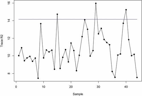
Figure 4. Monitoring ZA fertilizer production dataset using conventional GV control chart

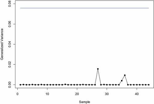
According to the figures, it can be seen that the proposed chart can detect the changes in the covariance matrix by declaring three out-of-control samples. Meanwhile, the conventional GV chart did not detect any out of control signal. Furthermore, the conventional method produces very small and similar statistics. This fact can be proved that the proposed chart is more sensitive to detect changes in the covariance matrix than the conventional one. Also, this is confirmed the second drawback of the conventional method that is the multivariate variability becomes small due to the quality characteristic is a linear combination of the other variables.

6. Conclusion

In this paper, the Tr(R²) control chart based on the squared correlation matrix with the trace operator is proposed in order to overcome the drawbacks of the existing multivariate variability chart. Kernel Density Estimation method is used to calculate the better control limit for the proposed chart. The simulation studies show that for the several combinations of a number of quality characteristics p and number of sample size n, the control limit using the KDE method always results in an ARL₀ at about 370 for $α = 0.00273$ . For $α \neq 0.00273,$ the proposed chart has ARL₀ near to $\frac{1}{α} .$ For the shifted process, the proposed chart demonstrated the great performance as shown by the ARL₁ value. The performance of the proposed chart becomes better for the larger number of quality characteristics and the number of sample size n in the process. The application of the proposed chart to monitor the ZA fertilizer production dataset shows that the proposed chart has a better performance to monitor the covariance matrix than the GV chart. For future research, the proposed chart will be applied to detect high dimensional big data due to its great ability for such a case. In addition, the use of the bootstrap resampling method is also appropriate for estimating the control limit of the proposed chart.

Disclosure statement

The authors declare that there are no potential conﬂict of interest

Additional information

Funding

The authors received no direct funding for this research.

Notes on contributors

Muhammad Mashuri

The corresponding author, Dr. Muhammad Mashuri is an associate professor in the Department of Statistics, Institut Teknologi Sepuluh Nopember, Surabaya Indonesia. His research interest includes statistical quality control and multivariate analysis, especially in industrial field. Haryono, Diaz Fitra Aksioma, and Wibawati are senior lecturers whose research interest includes statistical process control. Hidayatul Khusna and Muhammad Ahsan are PhD students through Master Program of Education Leading to Doctoral Degree for Excellent Graduates, an accelerated program for undergraduate prepared to be candidate lecturers or researchers with doctoral degrees.

References

Abbasi, S. A., & Miller, A. (2012). On proper choice of variability control chart for normal and non-normal processes. Quality and Reliability Engineering International, 28(3), 279–37. doi:10.1002/qre.1244
Web of Science ®Google Scholar
Abu‐Shawiesh, M. O. A., Kibria, G., & George, F. (2014). A robust bivariate control chart alternative to the Hotelling’s T2 Control Chart. Quality and Reliability Engineering International, 30(1), 25–35. doi:10.1002/qre.1474
Web of Science ®Google Scholar
Ahsan, M., Mashuri, M., & Khusna, H. (2017). Evaluation of Laney p’ Chart Performance. International Journal of Applied Engineering Research, 12(24), 14208–14217.
Google Scholar
Ahsan, M., Mashuri, M., Kuswanto, H., Prastyo, D. D., & Khusna, H. (2018a). Multivariate control chart based on PCA mix for variable and attribute quality characteristics. Production & Manufacturing Research, 6(1), 364–384. doi:10.1080/21693277.2018.1517055
Web of Science ®Google Scholar
Ahsan, M., Mashuri, M., Kuswanto, H., Prastyo, D. D., & Khusna, H. (2018b). T2 control chart based on successive difference covariance matrix for intrusion detection system. In Journal of Physics: Conference Series, Makassar, Indonesia (Vol. 1028, p. 12220). IOP Publishing.
Google Scholar
Alfaro, J. L., & Ortega, J. F. (2009). A comparison of robust alternatives to Hotelling’s T2 control chart. Journal of Applied Statistics, 36(12), 1385–1396. doi:10.1080/02664760902810813
Web of Science ®Google Scholar
Ali, H., Syed Yahaya, S. S., & Omar, Z. (2013). Robust hotelling T2 control chart with consistent minimum vector variance. Mathematical Problems in Engineering, 2013, 1–7. doi:10.1155/2013/401350
Web of Science ®Google Scholar
Alkindi, M., & Prastyo, D. D. (2016). T2 hotelling fuzzy and W2 control chart with application to wheat flour production process. In AIP Conference Proceedings, Yogyakarta, Indonesia (Vol. 1746). Doi:10.1063/1.4953977
Google Scholar
Alt, F. B., & Smith, N. D. (1988). Multivariate process control. Handbook of Statistics, 7, 333–351.
Web of Science ®Google Scholar
Amdouni, A., Castagliola, P., Taleb, H., & Celano, G. (2015). Monitoring the coefficient of variation using a variable sample size control chart in short production runs. The International Journal of Advanced Manufacturing Technology, 81(1), 1–14. doi:10.1007/s00170-015-7084-4
Web of Science ®Google Scholar
Amdouni, A., Castagliola, P., Taleb, H., & Celano, G. (2017). A variable sampling interval Shewhart control chart for monitoring the coefficient of variation in short production runs. International Journal of Production Research, 55(19), 5521–5536. doi:10.1080/00207543.2017.1285076
Web of Science ®Google Scholar
Aparisi, F., Jabaioyes, J., & Carrion, A. (1999). Statistical properties of the lsi multivariate control chart. Communications in Statistics - Theory and Methods, 28(11), 2671–2686. doi:10.1080/03610929908832445
Web of Science ®Google Scholar
Aparisi, F., Jabaloyes, J., & Carrión, A. (2001). GENERALIZED VARIANCE CHART DESIGN WITH ADAPTIVE SAMPLE SIZES. THE BIVARIATE CASE. Communications in Statistics - Simulation and Computation, 30(4), 931–948. doi:10.1081/SAC-100107789
Web of Science ®Google Scholar
Arkat, J., Niaki, S. T. A., & Abbasi, B. (2007). Artificial neural networks in applying MCUSUM residuals charts for AR(1) processes. Applied Mathematics and Computation, 189(2), 1889–1901. doi:10.1016/j.amc.2006.12.081
Web of Science ®Google Scholar
Burden, R. L., & Faires, J. D. (2011). Numerical analysis. Cengage learning. USA. doi:10.1017/CBO9781107415324.004
Google Scholar
Calzada, M. E., & Scariano, S. M. (2013). A synthetic control chart for the coefficient of variation. Journal of Statistical Computation and Simulation, 83(5), 853–867. doi:10.1080/00949655.2011.639772
Web of Science ®Google Scholar
Castagliola, P., Achouri, A., Taleb, H., Celano, G., & Psarakis, S. (2015). Monitoring the coefficient of variation using a variable sample size control chart. The International Journal of Advanced Manufacturing Technology, 80(9), 1561–1576. doi:10.1007/s00170-015-6985-6
Web of Science ®Google Scholar
Castagliola, P., Celano, G., & Psarakis, S. (2011). Monitoring the Coefficient of Variation Using EWMA Charts. Journal of Quality Technology, 43(3), 249–265. doi:10.1080/00224065.2011.11917861
Web of Science ®Google Scholar
Chatterjee, S., & Hadi, A. S. (2009). Sensitivity analysis in linear regression (Vol. 327). New York, NY: John Wiley & Sons.
Google Scholar
Chen, G., CHENG, S. W., & Xie, H. (2005). A new multivariate control chart for monitoring both location and dispersion. Communications in Statistics—Simulation and Computation®, 34(1), 203–217. doi:10.1081/SAC-200047087
Web of Science ®Google Scholar
Chou, Y.-M., Mason, R., & Young, J. (2001). The control chart for individual observations from a multivariate non-normal distribution. Communications in Statistics: Theory & Methods, 30(8/9), 1937. doi:10.1081/STA-100105706
Web of Science ®Google Scholar
Costa, A. F. B., & Machado, M. A. G. (2009). A new chart based on sample variances for monitoring the covariance matrix of multivariate processes. The International Journal of Advanced Manufacturing Technology, 41(7), 770–779. doi:10.1007/s00170-008-1502-9
Web of Science ®Google Scholar
Costa, A. F. B., & Machado, M. A. G. (2011). A control chart based on sample ranges for monitoring the covariance matrix of the multivariate processes. Journal of Applied Statistics, 38(2), 233–245. doi:10.1080/02664760903406413
Web of Science ®Google Scholar
Croux, C., & Haesbroeck, G. (1999). Influence function and efficiency of the minimum covariance determinant scatter matrix estimator. Journal of Multivariate Analysis, 71(2), 161–190. doi:10.1006/jmva.1999.1839
Web of Science ®Google Scholar
Djauhari, A. M. (2005a). Improved monitoring of multivariate process variability. Journal of Quality Technology, 37(1), 32–39. Retrieved from http://proquest.umi.com/pqdweb?did=773835061&Fmt=7&clientId=3740&RQT=309&VName=PQD
Web of Science ®Google Scholar
Djauhari, M. A. (2005b). Outlier detection: Some challenging problem for future research. Proceedings of the Eighth Islamic Countries Conference on Statistical Sciences, National University of Computer and Emerging Sciences, Lahore.
Google Scholar
Djauhari, M. A. (2010). A multivariate process variability monitoring based on individual observations. Modern Applied Science, 4(10), 91. doi:10.5539/mas.v4n10p91
Google Scholar
Doǧu, E., & Kocakoç, İ. D. (2011). Estimation of change point in generalized variance control chart. Communications in Statistics - Simulation and Computation, 40(3), 345–363. doi:10.1080/03610918.2010.542844
Web of Science ®Google Scholar
Gadre, M. P., & Kakade, V. C. (2018). Two group inspection-based control charts for dispersion matrix. Communications in Statistics - Simulation and Computation, 47(6), 1652–1669. doi:10.1080/03610918.2017.1321120
Web of Science ®Google Scholar
Grambow, S. C., & Stromberg, A. J. (1998). Combining the EID and FSA for computing the minimum volume ellipsoid. Deptartment of Stats., University of Kentucky.
Google Scholar
Grigoryan, A., & He, D. (2005). Multivariate double sampling |S| Charts for controlling process variability. International Journal of Production Research, 43(4), 715–730. doi:10.1080/00207540410001716525
Web of Science ®Google Scholar
Hamed, M. S. (2014). Generalized variance chart for multivariate quality control process procedure with application. Applied Mathematical Sciences, 8(163), 8137–8151. doi:10.12988/ams.2014.49734
Google Scholar
Härdle, W., & Linton, O. (1994). Applied nonparametric methods. Handbook of Econometrics, 4(26), 2295–2339. doi:10.1016/S1573-4412(05)80007-8
Google Scholar
Holmes, D. S., & Mergen, A. E. (1993). Improving the performance of the T2 control chart. Quality Engineering, 5(4), 619–625. doi:10.1080/08982119308919004
Google Scholar
Huwang, L., Yeh, A. B., & Wu, C.-W. (2007). Monitoring multivariate process variability for individual observations. Journal of Quality Technology, 39(3), 258–278. doi:10.1080/00224065.2007.11917692
Web of Science ®Google Scholar
Issam, B. K., & Mohamed, L. (2008). Support vector regression based residual MCUSUM control chart for autocorrelated process. Applied Mathematics and Computation, 201(1–2), 565–574. doi:10.1016/j.amc.2007.12.059
Web of Science ®Google Scholar
Kang, C. W., Lee, M. S., Seong, Y. J., & Hawkins, D. M. (2007). A control chart for the coefficient of variation. Journal of Quality Technology, 39(2), 151–158. doi:10.1080/00224065.2007.11917682
Web of Science ®Google Scholar
Khatun, M., Khoo, M. B. C., Lee, M. H., & Castagliola, P. (2018). One-sided control charts for monitoring the multivariate coefficient of variation in short production runs. Transactions of the Institute of Measurement and Control, 0142331218789481.
Web of Science ®Google Scholar
Khaw, K. W., Khoo, M. B. C., Yeong, W. C., & Wu, Z. (2017). Monitoring the coefficient of variation using a variable sample size and sampling interval control chart. Communications in Statistics - Simulation and Computation, 46(7), 5772–5794. doi:10.1080/03610918.2016.1177074
Web of Science ®Google Scholar
Khusna, H., Mashuri, M., Ahsan, M., Suhartono, S., & Prastyo, D. D. (2018). Bootstrap based maximum multivariate CUSUM control chart. Quality Technology & Quantitative Management, 1–23. doi:10.1080/16843703.2018.1535765
Web of Science ®Google Scholar
Khusna, H., Mashuri, M., Suhartono, P. D., & Ahsan, M. (2018). Multioutput least square SVR based multivariate EWMA control chart. Journal of Physics: Conference Series, 1028(1), 12221. Retrieved from http://stacks.iop.org/1742-6596/1028/i=1/a=012221
Google Scholar
Lee, M. H., & Khoo, M. B. C. (2017). Optimal designs of multivariate synthetic |S| Control chart based on median run length. Communications in Statistics - Theory and Methods, 46(6), 3034–3053. doi:10.1080/03610926.2015.1048884
Web of Science ®Google Scholar
Lee, M. H., & Khoo, M. B. C. (2018). Double sampling |S| Control chart with variable sample size and variable sampling interval. Communications in Statistics - Simulation and Computation, 47(2), 615–628. doi:10.1080/03610918.2017.1288246
Web of Science ®Google Scholar
Li, Z., & Tsung, F. (2019). A control scheme for monitoring process covariance matrices with more variables than observations. Quality and Reliability Engineering International, 35(1), 351–367. doi:10.1002/qre.2403
Web of Science ®Google Scholar
Lim, A. J. X., Khoo, M. B. C., Teoh, W. L., & Haq, A. (2017). Run sum chart for monitoring multivariate coefficient of variation. Computers & Industrial Engineering, 109, 84–95. doi:10.1016/j.cie.2017.04.023
Web of Science ®Google Scholar
Maboudou-Tchao, E. M., & Diawara, N. (2013). A LASSO chart for monitoring the covariance matrix. Quality Technology & Quantitative Management, 10(1), 95–114. doi:10.1080/16843703.2013.11673310
Web of Science ®Google Scholar
Machado, M. A. G., Costa, A. F. B., & Rahim, M. A. (2009). The synthetic control chart based on two sample variances for monitoring the covariance matrix. Quality and Reliability Engineering International, 25(5), 595–606. doi:10.1002/qre.992
Web of Science ®Google Scholar
Mashuri, M., Haryono, P., Wibawati, A. D. F., Khusna, H., & Ahsan, M. (2016). Trace R2 control chart for monitoring variability. In International Conference on Theoretical and Applied Statistics-Conference Proceedings, Surabaya, Indonesia.
Google Scholar
Montgomery, D. (2009). Introduction to statistical quality control. New York: John Wiley & Sons Inc. doi:10.1002/1521-3773(20010316)40:6<9823::AID-ANIE9823>3.3.CO;2-C
Google Scholar
Noorossana, R., & Vaghefi, S. J. M. (2006). Effect of autocorrelation on performance of the MCUSUM control chart. Quality and Reliability Engineering International, 22(2), 191–197. doi:10.1002/qre.695
Web of Science ®Google Scholar
Page, E. S. (1961). Cumulative sum charts. Technometrics, 3(1), 1–9. doi:10.1080/00401706.1961.10489922
Web of Science ®Google Scholar
Parzen, E. (1962). On estimation of a probability density function and mode. The Annals of Mathematical Statistics, 33(3), 1065–1076. doi:10.1214/aoms/1177704472
Google Scholar
Peña, D., & Rodrı́guez, J. (2003). Descriptive measures of multivariate scatter and linear dependence. Journal of Multivariate Analysis, 85(2), 361–374. doi:10.1016/S0047-259X(02)00061-1
Web of Science ®Google Scholar
Phaladiganon, P., Kim, S. B., Chen, V. C. P., Baek, J.-G., & Park, S.-K. (2011). Bootstrap-Based T 2 multivariate control charts. Communications in Statistics - Simulation and Computation, 40(5), 645–662. doi:10.1080/03610918.2010.549989
Web of Science ®Google Scholar
Phaladiganon, P., Kim, S. B., Chen, V. C. P., & Jiang, W. (2013). Principal component analysis-based control charts for multivariate nonnormal distributions. Expert Systems with Applications, 40(8), 3044–3054. doi:10.1016/j.eswa.2012.12.020
Web of Science ®Google Scholar
Pirhooshyaran, M., & Niaki, S. T. A. (2015). A double-max MEWMA scheme for simultaneous monitoring and fault isolation of multivariate multistage auto-correlated processes based on novel reduced-dimension statistics. Journal of Process Control, 29, 11–22. doi:10.1016/j.jprocont.2015.03.008
Web of Science ®Google Scholar
Riaz, M. (2008). A dispersion control chart. Communications in Statistics - Simulation and Computation, 37(6), 1239–1261. doi:10.1080/03610910802049623
Web of Science ®Google Scholar
Riaz, M., & Does, R. J. M. M. (2008). An alternative to the bivariate control chart for process dispersion. Quality Engineering, 21(1), 63–71. doi:10.1080/08982110802445579
Web of Science ®Google Scholar
Roberts, S. W. (1959). Control chart tests based on geometric moving averages. Technometrics, 1(3), 239–250. doi:10.1080/00401706.1959.10489860
Google Scholar
Rosenblatt, M. (1956). Remarks on some nonparametric estimates of a density function. The Annals of Mathematical Statistics, Volume, 27, 832–837. doi:10.1214/aoms/1177728190
Google Scholar
Shewhart, W. A. (1924). Some applications of statistical methods to the analysis of physical and engineering data. Bell Labs Technical Journal, 3(1), 43–87. doi:10.1002/j.1538-7305.1924.tb01347.x
Google Scholar
Sindelar, M. F. (2007). Multivariate statistical process control for correlation matrices. University of Pittsburgh.
Google Scholar
Suwanda, & Djauhari, A. M. (2003). A new concept in monitoring multivariate process variability. Data Analysis Research Group, 2(2), 1–2.
Google Scholar
Tang, P. F., & Barnett, N. S. (1996). Dispersion control for multivariate processes. Australian Journal of Statistics, 38(3), 235–251. doi:10.1111/anzs.1996.38.issue-3
Google Scholar
Wibawati, M., Purhadi, M., & Ahsan, M. (2018). Perfomance fuzzy multinomial control chart. Journal of Physics: Conference Series, 1028(1), 12120. Retrieved from http://stacks.iop.org/1742-6596/1028/i=1/a=012120
Google Scholar
Wibawati, M., Purhadi, M., & Irhamah. (2016). Fuzzy multinomial control chart and its application. In AIP Conference Proceedings, Surabaya, Indonesia (Vol. 1718). doi:10.1063/1.4943351
Google Scholar
Yeh, A. B., Huwang, L., & Wu, C.-W. (2005). A multivariate EWMA control chart for monitoring process variability with individual observations. IIE Transactions, 37(11), 1023–1035. doi:10.1080/07408170500232263
Web of Science ®Google Scholar
Yeong, W. C., Khoo, M. B. C., Teoh, W. L., & Castagliola, P. (2016). A control chart for the multivariate coefficient of variation. Quality and Reliability Engineering International, 32(3), 1213–1225. doi:10.1002/qre.1828
Web of Science ®Google Scholar
Yeong, W. C., Khoo, M. B. C., Tham, L. K., Teoh, W. L., & Rahim, M. A. (2017). Monitoring the coefficient of variation using a variable sampling interval EWMA chart. Journal of Quality Technology, 49(4), 380–401. doi:10.1080/00224065.2017.11918004
Web of Science ®Google Scholar

Appendix dataset

Table

Download CSV Display Table

Tr(R²) control charts based on kernel density estimation for monitoring multivariate variability process