Applying boundary element method to simulate a high-skew Controllable Pitch Propeller with different hub diameters for preliminary design purposes

Abstract

Using the controllable pitch propeller (CPP) in marine propulsion system makes it possible to have maximum ship speed and low fuel consumption at different engine rpm. Good maneuverability is another advantage of such propeller. This feature has persuaded designers to use CPP in ships with various mission profiles like tugs or ferries. The hub boss is of great importance in CP Propellers because it provides housing for blade actuation mechanism. On the other hand, hub boss geometry should be selected as small as possible since it has negative effect on hydrodynamic performance of propeller, specially its thrust and efficiency. In this article, a 3D potential flow-based solver is developed to predict the hydrodynamic characteristic of marine propellers for preliminary and basic design purposes. Through applying the time stepping scheme, it is possible to generate the rollup wake pattern at each time step. As a result, the interaction of vortex wake-lifting/non-lifting bodies are correctly taken into consideration. Validation of the proposed numerical model is carried out with two standard marine propellers (DTMB4119 and KP505) and a high skewed B-series Controllable Pitch Propeller (CPP). Subsequently, a series of parametric simulations are performed on different non-dimensional hub diameters of a CP propeller to find an appropriate hub diameter (big enough to provide CPP mechanism) with highest propeller performance. Ultimately, the suitable hub diameter is determined for an appropriate design of a CP propeller.

Rollup pattern for the RV propeller with different hub diameters.

Keywords:

• Boundary element method
• time stepping method
• wake sheet generation
• twin propeller
• multi-body simulation

PUBLIC INTEREST STATEMENT

Using the controllable pitch propeller (CPP) in marine propulsion system makes it possible to have maximum ship speed and low fuel consumption at different engine rpm. Good maneuverability is another advantage of such propeller. This feature has persuaded designers to use CPP in ships with various mission profiles like tugs or ferries. The hub boss is of great importance in CP Propellers because it provides housing for blade actuation mechanism. On the other hand, hub boss geometry should be selected as small as possible since it has negative effect on hydrodynamic performance of propeller, specially its thrust and efficiency. In this article, a 3D potential flow-based solver is developed to predict the hydrodynamic characteristic of marine propellers for preliminary and basic design purposes. As a result, rollup wake pattern at each time step is generated while interaction of vortex wake-lifting/non-lifting bodies are considered. Ultimately, an optimum hub diameter with highest propeller performance is determined for an appropriate design of a CP propeller.

1. Introduction

Prediction of propeller performance has been traditionally centered on ship propulsion’s design, especially in basic and preliminary phases. For this purpose, numerical simulations are very popular related to expensive and time-consuming solutions like experimental test. Finite Volume Method (FVM) is a common approach by which many commercial software (or personal codes methods) are developed to simulate hydrodynamic problems. This method is based on volumetric grids and simulation of moving object requires special techniques such as moving grid or overset methods (Benek et al., 1983; Henshaw & Schwendeman, 2006; Meakin & Suhs, 1989) which increases the computational time, significantly. Felice et al. (2009) investigated the performance of a seven-blade propeller of a submarine (model E1619 designed by INSEAN), using experimental and computational methods. The computational method was based on Large Eddy Simulation (LES) and the velocity was measured using Laser Doppler Velocimetry (LDV). Bennaya et al. (2013) used a commercial numerical FVM model (FLUENT) to simulate a conventional screw propeller DTRC P4119. They tried to find an appropriate method to calculate hydrodynamic performance ($K_T,K_Q$) of the propeller and compared them with existing experimental data. Dubbioso et al. (2013) developed a numerical code on unsteady RANS equations to simulate marine propeller (CNR-INSEAN E779A) which worked in oblique flow condition. For this purpose, they used a dynamically overlapping grid approach and mainly focused on hydrodynamic loads (including forces and moments) that act on the blade, hub and the complete propeller. Wang et al. (2018) numerically examined the characteristics of the relationship between skew angle of four different five-blade DTMB propeller and evolution of trailing vortex wake. They used the RANS based commercial software STAR-CCM+ to perform the numerical analysis. Their result showed that by increasing the propeller skew angle, the deformation of the hub vortex and destabilization of the tip vortices weaken, gradually. They also showed that increasing the skew angle can reduce the difference in trailing vortex wake contraction under various loading conditions.

Despite the good accuracy of RANS based solvers, since they are known to be very time consuming in simulations, scientists tried to use and develop faster approaches, especially in preliminary and basic design stage. For example, Gaafary et al. (2011) developed a computer code to find the optimum characteristics of B-Series marine Propellers. The design algorithm was performed as a single objective function subjected to constraints imposed by other parameters like cavitation, propeller thrust and even material strength. Although this computational process was based on the propeller series diagrams or regression polynomials, they showed that it can be very useful tool for basic/preliminary design purposes, due to its low computation time.

On the other hand, Boundary Element Method (BEM) is another classic approach which has widely been developed in recent decade to simulate hydrodynamic problems, especially the ones with lifting bodies such as foils and propellers. One of the most important advantage of BEM over the common CFD approaches such as FEM or FVM is the fact that it can offer a better accuracy to computational time ratio. Although BEM is a potential flow-based method which incapable of calculating viscous force, but it can still widely be used in basic design and preliminary estimations, due to its low computational time. Another benefit which has led researchers to adopt BEM method for their simulations, is its simple implementation in modelling two or more objects with different moving frames. This is due to the fact that BEM uses surface grids which are not intertwined with each other like the volumetric grid methods.

The first researchers who used boundary element method to simulate flow around arbitrary bodies were Hess and Smith (Hess & Smith, 1962). Subsequently, Hess and Valarezo (1985) used Hess’s classical formulations (Hess, 1972) and developed a way to simulate flow around marine propeller in steady state condition. They used Prescribed Wake Shape (PWS) method to simulate the emanating trailing vortex at the trailing edge of each blade. Politis (2004) has also applied Time Stepping Method (TSM) and developed a BEM code to capture the vortex sheet. He simulated unsteady motion of a DTMB4119 marine propeller and showed that BEM has very good performance predicting forces and pressure distributions. In 2011 (Politis, 2011), he applied his solver to a wide range of working conditions of a propeller, such as propeller in straight/circular course, azimuth propeller, and ducted propeller in circular course. He also showed that burst starting of a propeller may be modeled with good agreement through his method, compared with experimental data. Greco et al. (2014) investigated the capabilities of a boundary element method for the analysis of marine propeller hydrodynamics through comparison with RANS simulations and experimental data. They applied BEM model to INSEAN E779A right-handed marine propeller. The results showed good agreements with RANS computations and experimental data, albeit beneath the design working point, an overall worsening of BEM result is observed. This is due to the fact that more complex shape of the rolled-up wake makes the wake alignment procedure prone to numerical instabilities during the solution convergence. In 2017, Rahman et al. (2017) presented a design method based on lifting line theory and lifting surface correction factors for marine propellers. They applied this method for a US Navy combat DTMB 5415 ship. They showed that the presented method gives good results (including hydrodynamic pitch, Circulation, Pitch-Diameter ratio and Camber-Chord ratio) compared to practical data. Najafi & Abbaspoor, (2017) presented a BEM solver to simulate submerged marine propellers. They imposed a smoothing function to damp the effect of singularities due to inherent instability of the boundary integral equations. The effect of this scheme with different constants was investigated through modeling a high skew marine propeller DTMB 4284 with hub. In 2010, Gaggero et al. (2010) tried to compare a commercial RANS solver (StarCCM+) with a house developed panel method, in simulating DTMB 4679 propeller. Panel method completed a simulation in about 40 min on a single processor while RANS solved the same test case in about 5 h on a 12 processors cluster. Results showed that the panel method is an efficient tool to predict unsteady force and also pressure distribution on blades. Ultimately, they suggested that panel method be used in basic designs problems while RANS solver is the optimized design validation method. Meanwhile, Brizzolara et al. (2008) performed an extensive study regarding the quality of the results of RANS and BEM methods in propeller modelling. They simulated five standard propellers and compared all global (thrust/torque) and local (pressure distribution on blades) hydrodynamic characteristics of the propellers. They showed that both methods could be used for design purposes with sufficient accuracy (within 2–3%). They also concluded that at design advance coefficient, pressure distribution is very similar, but as expected, RANS solver demonstrates better accuracy at low advance ratio. In order to find more efficient method to analyze off-design aspects related to the ship and its propulsion system in the earlier design stages, Gaggero et al. (2019) in 2019 investigated the capability of BEM and Blade Element (BEMT) propeller solver to predict the propeller performance in maneuvering condition. Comparison between BEM and BEMT was conducted for he behind hull condition of a twin-screw ship. It was found that however BEM is, it is at least one order slower than BEMT. However, it was more accurate and could predict the propeller performance behind the ship with acceptable accuracy. In 2020, Miglianti et al. (2020) tried to develop a tool to predict the cavitation in marine propeller at design stage. For this purpose, they used a model based on a dataset which was collected on cavitation tunnel and a numerical solver based on boundary element method.

1.1. Hub influence on CPP

It is well known that among marine propellers, controllable pitch propellers are very popular for special ships like sailing, passengers, or tugs because of its good maneuverability and high efficiency at different working conditions. One of the main concerns in designing and manufacturing the CP propellers is selecting a suitable hub diameter. Hub provides a housing for pitch change mechanism, but on the other hand since hub is not a lifting body, the bigger hub would increase the total viscosity drag and therefore reduces the propeller thrust. Based on comparison of two fixed and CP propeller with the same overall diameters, it could be concluded that the fixed pitch propeller would generate more thrust because it has smaller hub and thus more expanded area. There are several works which have investigated hub effect on propeller performance.

Shamsi et al. (2014) evaluated the propulsive performance of a marine propeller with different hub taper angle. They used a Reynolds-Averaged Navier Stokes (RANS) commercial solver (Fluent 6.3) combined with Moving Reference Frame (MRF) technique (in order to simulate moving bodies) for all simulations. They first verified the method by a single propeller (with different hub taper angle) and compared the result with experimental data. Subsequently, the method was applied to the podded drive unit for both puller and pusher configuration. It was shown that there is good agreement between the experimental measurements and numerical method. Lim et al. (2014) examined the design parameters of a Propeller Boss Cap Fin (PBCF) and hub cap for a container ship to improve the propeller efficiency. They used a commercial CFD tool (Ansys CFX 14.0) and validated the results with a propeller open water test. Their results showed that the pitch and chord to span ratio are two main parameters which affect the propeller efficiency more than other design parameters. It is also shown that the hub vortex downstream of the propeller increases the propeller torque which leads to a decrease in the performance. song et al. (2015) investigated the open water performance of the Rim Driven Thruster (RDT) by means of a commercial Computational Fluid Dynamic (CFD) code, CFX 14.0. In this work, they determined the difference between hub-type and hubless type RDT in four different hub radii. Based on the computational results, it was concluded that hubless RDT has a higher efficiency than the hub-type RDT.

1.2. Motivation of this work

In this paper, a numerical in-house code which is based on BEM method, is developed to simulate unsteady flow around a marine Controllable Pitch Propeller (CPP). Based on the presented literature review, one of the main reasons for choosing the potential flow over RANS solvers is that BEM solvers have higher performance in computational time which is very useful in preliminary/basic design. This solver is designed to investigate the hydrodynamic performance of a CPP with different hub diameters to find a proper diameter which not only provides appropriate housing for CP propeller, but also supply acceptable performance.

In the present solver, each propeller is supposed to consist of lifting bodies (blades) and a non-lifting body (hub). The Time Stepping Method (TSM) is used to simulate the freely moving unsteady trailing vortex sheet which emanates from trailing edge of each blade. The proposed numerical solver is validated with two standard benchmark and a practical test case. The standard test cases include a DTMB4119 and KP505 marine propeller, while the practical example is a high skew B-series CPP which is used in a research vessel. The acquired numerical results are compared with experimental data. After validation, the solver is used to parametrically study the effect of hub diameter on the high skewed CPP performance, including${\mathrm{K}}_{\mathrm{T}},{\mathrm{K}}_{\mathrm{Q}},\eta$. Through this parametric study, a proper hub diameter can be selected for changing pitch mechanism, especially in preliminary design purpose.

2. Governing equation

Boundary element method is based on potential flow which depends on three main assumptions: incompressible, irrotational, non-viscous flow. Accordingly, velocity is described as velocity potential $\varphi \left(x,t\right)$ and should satisfy the three-dimensional Laplace equation.

(1) ${\mathrm{\nabla }}^2\varphi =0$(1)

The total potential velocity $\varphi \left(x,t\right)$ can be written as a linear combination of fundamental potential functions such as sink/source, dipole and vortex which could be compute on each cell (all types of cells are identified in the followings). By applying the Green’s second identity, one could write the Laplace equation for any $x$, located on the cell center in the following form:

(2) $2\pi \varphi \left(x,t\right)=\underset{\mathrm{S}}{\overset{\hspace{0.17em}}{\int }}\varphi \left(x,t\right)\frac{\mathrm{\partial }\lambda }{\mathrm{\partial }n}dS+\underset{\mathrm{S}}{\overset{\hspace{0.17em}}{\int }}\lambda \frac{\mathrm{\partial }\varphi \left(x,t\right)}{\mathrm{\partial }n}dS$(2)

where $\lambda$ is defined as fundamental solution for potential flow. In 3D formulation, $\lambda =\frac{1}{r}$ and $n$ is the unit normal vector of panel, pointing outward of body and $\mathrm{r}$ represents the distance between the source point and the field point.

As a result, Equation (2)(2) $2\pi \varphi \left(x,t\right)=\underset{\mathrm{S}}{\overset{\hspace{0.17em}}{\int }}\varphi \left(x,t\right)\frac{\mathrm{\partial }\lambda }{\mathrm{\partial }n}dS+\underset{\mathrm{S}}{\overset{\hspace{0.17em}}{\int }}\lambda \frac{\mathrm{\partial }\varphi \left(x,t\right)}{\mathrm{\partial }n}dS$(2) can be written in the form of

(3) $2\pi \varphi \left(x,t\right)-\underset{S_W+S_B}{\overset{\hspace{0.17em}}{\int }}\varphi \left(y,t\right)\frac{\mathrm{\partial }\left(\frac{1}{r}\right)}{\mathrm{\partial }n}dS=\underset{S_W+S_B}{\overset{\hspace{0.17em}}{\int }}\frac{1}{r}\frac{\mathrm{\partial }\varphi \left(y,t\right)}{\mathrm{\partial }n}dS$(3)

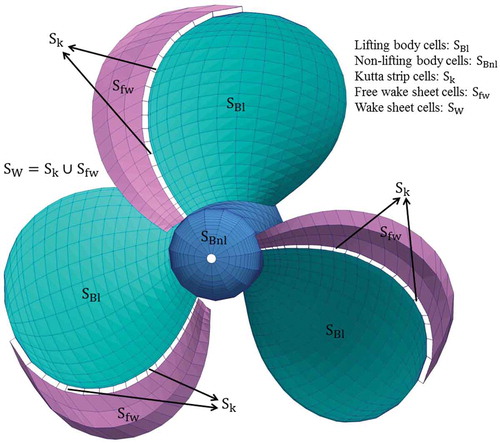
In the presented formulation, for the simplicity and better understanding, the discretized domain has been divided in four different zones, and each cell in the zones, is treated differently according to the main equation:

1- Lifting cells ($S_{Bl}$): all the cells on each propeller contribute to generating the lifting force. The wake sheet is generated from the first time step, next to the lifting cells (clause no. 3).

2- Non-lifting cells ($S_{Bnl}$): all the cells on hub and propeller cylinder, these cells are NOT contributed to generating the lifting force.

3- Kutta-strip cells ($S_k$): The first row of cells in the wake sheet which are adjacent to the trailing edges of the lifting body.

4- Free wake sheet cells ($S_{fw}$): Other cells on the wake sheet.

These zones are shown in Figure 1. As illustrated, the wake sheet ($S_W=S_k{\cup }^{S_{fw}}$) consists of two different zones, as described in clauses 2 and 3 (above).

Figure 1. Cell types in the propeller.

The dipole intensity ($\mu$) for all free wake sheet cells are known from the previous time step, while the intensity over Kutta-strip cells are unknown.

Equation (4)(4) $2\pi \varphi \left(x,t\right)+\text{ mathop {}\sum \text{^ }limits\_}{S}_B\varphi \left(x,t\right)\text{{}\int \text{^ ^}{}\frac{\overrightarrow{n}.\overrightarrow{r}}{r^3}dS+\text{ mathop {}\sum \text{^ }limits\_}{S}_k\mu \left(x,t\right)\text{{}\int \text{^ ^}{}\frac{\overrightarrow{n}.\overrightarrow{r}}{r^3}dS=\text{ mathop {}\sum \text{^ }limits\_}{S}_B\text{ {}\int \text{^ ^}{}\frac{\overrightarrow{n}.\overrightarrow{q}}{r}dS-\text{ mathop {}\sum \text{^ }limits\_}{S}_{fw}\text{ {}\int \text{^ ^}}\mu \text{ {}\frac{\overrightarrow{n}.\overrightarrow{r}}{r^3}dS$(4) shows the discretized form of Equation (3)(3) $2\pi \varphi \left(x,t\right)-\underset{S_W+S_B}{\overset{\hspace{0.17em}}{\int }}\varphi \left(y,t\right)\frac{\mathrm{\partial }\left(\frac{1}{r}\right)}{\mathrm{\partial }n}dS=\underset{S_W+S_B}{\overset{\hspace{0.17em}}{\int }}\frac{1}{r}\frac{\mathrm{\partial }\varphi \left(y,t\right)}{\mathrm{\partial }n}dS$(3) (Politis, 2011):

(4) $2\pi \varphi \left(x,t\right)+\text{ mathop {}\sum \text{^ }limits\_}{S}_B\varphi \left(x,t\right)\text{{}\int \text{^ ^}{}\frac{\overrightarrow{n}.\overrightarrow{r}}{r^3}dS+\text{ mathop {}\sum \text{^ }limits\_}{S}_k\mu \left(x,t\right)\text{{}\int \text{^ ^}{}\frac{\overrightarrow{n}.\overrightarrow{r}}{r^3}dS=\text{ mathop {}\sum \text{^ }limits\_}{S}_B\text{ {}\int \text{^ ^}{}\frac{\overrightarrow{n}.\overrightarrow{q}}{r}dS-\text{ mathop {}\sum \text{^ }limits\_}{S}_{fw}\text{ {}\int \text{^ ^}}\mu \text{ {}\frac{\overrightarrow{n}.\overrightarrow{r}}{r^3}dS$(4)

The intensity of source distribution for body cells (first term on the right-hand side) is known at each time step and is calculated numerically (Najafi & Abbaspour, 2017). The second term on the right-hand side can also be calculated for all the free wake cells, since the dipole intensity and the free wake shape are known from the previous step. As pointed out earlier, the Kutta strip would impose additional unknown to the problem. These extra unknowns would be satisfied as stated in the following boundary condition section. Calculating the influence coefficients yield a system of equations ($\mathrm{A}\mathrm{X}=\mathrm{B}$) which may be solved by common iterative methods like successive over relaxation (SOR) scheme. The solution is a doublet intensity distribution over the lifting and non-lifting bodies.

2.1. Boundary conditions

In order to complete the influence coefficient, some conditions are applied on the boundaries. The first one is no flux kinematic boundary condition which is defined as follows (Zhu et al., 2002):

(5) $\frac{\mathrm{\partial }\varphi \left(x,t\right)}{\mathrm{\partial }n}=\left\{\overrightarrow{{\mathit{V}}_b}\left(x,t\right)-\overrightarrow{\mathbf{\nabla }{\varphi }_w}\left(x,t\right)\right\}.\overrightarrow{n}$(5)

where $\overrightarrow{V_b}\left(x,t\right)$ is the prescribed propeller velocity. The second one, Equation (6)(6) ${\varphi }_{uppercells}-{\varphi }_{lowercells}=\mu$(6) is Kutta condition which is applied for lifting bodies with trailing edges. At the trailing edge, flow should leave the body smoothly with finite velocity and without any pressure jump. In this paper, by applying a linear Morino-type Kutta condition (Politis, 2011) at any time step, the dipole intensity of Kutta-strip cells (the third term in LHS of Equation (4)(4) $2\pi \varphi \left(x,t\right)+\text{ mathop {}\sum \text{^ }limits\_}{S}_B\varphi \left(x,t\right)\text{{}\int \text{^ ^}{}\frac{\overrightarrow{n}.\overrightarrow{r}}{r^3}dS+\text{ mathop {}\sum \text{^ }limits\_}{S}_k\mu \left(x,t\right)\text{{}\int \text{^ ^}{}\frac{\overrightarrow{n}.\overrightarrow{r}}{r^3}dS=\text{ mathop {}\sum \text{^ }limits\_}{S}_B\text{ {}\int \text{^ ^}{}\frac{\overrightarrow{n}.\overrightarrow{q}}{r}dS-\text{ mathop {}\sum \text{^ }limits\_}{S}_{fw}\text{ {}\int \text{^ ^}}\mu \text{ {}\frac{\overrightarrow{n}.\overrightarrow{r}}{r^3}dS$(4) is achieved:

(6) ${\varphi }_{uppercells}-{\varphi }_{lowercells}=\mu$(6)

2.2. Wake sheet equation

Wake sheet is defined as an infinitesimal thickness layer. As mentioned before, the dipole intensity over Kutta strip is calculated at each time step while the intensity of other cells supposed to be known from previous time step. In the Time Stepping Method, it is necessary to generate a new row of nodes on each wake sheet (for each blade) and also calculate the new position of the previous nodes. For this purpose, the mean perturbation velocities ($\overrightarrow{{\nu }_m}$) on free vortex sheet should be calculated and subsequently, the new position of the nodes could be achieved by applying the Euler-Forward Scheme (EF Scheme) as follows (Zhu et al., 2002):

(7) $\overrightarrow{X_{new}}=\overrightarrow{X_{old}}+\left(\overrightarrow{{\nu }_m}.dt\right)+\overrightarrow{V_{rel}}.dt$(7)

$\overrightarrow{V_{rel}}$ is computed from Equation (11)(11) $V_{rel}=\overrightarrow{V}\left(t\right)\to \overrightarrow{\mathrm{\Omega }}\left(t\right)\times \overrightarrow{r}.$(11) . Based on this formula, the first-order wake alignment method is used to ensure that the wake is locally tangent to the direction of the flow. The third term on the right-hand side represents the relative velocity of each panel. Since the propeller rotates ($\left(t\right)$: angular velocity) and there is also a free downstream velocity, the relative velocity is of great importance in all equations.

Taking gradient from Equation (4)(4) $2\pi \varphi \left(x,t\right)+\text{ mathop {}\sum \text{^ }limits\_}{S}_B\varphi \left(x,t\right)\text{{}\int \text{^ ^}{}\frac{\overrightarrow{n}.\overrightarrow{r}}{r^3}dS+\text{ mathop {}\sum \text{^ }limits\_}{S}_k\mu \left(x,t\right)\text{{}\int \text{^ ^}{}\frac{\overrightarrow{n}.\overrightarrow{r}}{r^3}dS=\text{ mathop {}\sum \text{^ }limits\_}{S}_B\text{ {}\int \text{^ ^}{}\frac{\overrightarrow{n}.\overrightarrow{q}}{r}dS-\text{ mathop {}\sum \text{^ }limits\_}{S}_{fw}\text{ {}\int \text{^ ^}}\mu \text{ {}\frac{\overrightarrow{n}.\overrightarrow{r}}{r^3}dS$(4) (Politis, 2004), it can be written

(8) $\overrightarrow{{\nu }_m}=\frac{1}{4\pi }\underset{S}{\overset{\hspace{0.17em}}{\int }}\left(\overrightarrow{n}.\overrightarrow{\mathrm{\nabla }\varphi }\right)\overrightarrow{\frac{r}{r^3}}ds+\frac{1}{4\pi }\underset{S}{\overset{\hspace{0.17em}}{\int }}\left(\overrightarrow{n}\times \overrightarrow{\mathrm{\nabla }\varphi }\right)\times \overrightarrow{\frac{r}{r^3}}ds-\frac{1}{4\pi }\underset{L}{\overset{\hspace{0.17em}}{\int }}\varphi \frac{\overrightarrow{dl}\times \overrightarrow{r}}{r^3}ds$(8)

The discretized form of Equation (8)(8) $\overrightarrow{{\nu }_m}=\frac{1}{4\pi }\underset{S}{\overset{\hspace{0.17em}}{\int }}\left(\overrightarrow{n}.\overrightarrow{\mathrm{\nabla }\varphi }\right)\overrightarrow{\frac{r}{r^3}}ds+\frac{1}{4\pi }\underset{S}{\overset{\hspace{0.17em}}{\int }}\left(\overrightarrow{n}\times \overrightarrow{\mathrm{\nabla }\varphi }\right)\times \overrightarrow{\frac{r}{r^3}}ds-\frac{1}{4\pi }\underset{L}{\overset{\hspace{0.17em}}{\int }}\varphi \frac{\overrightarrow{dl}\times \overrightarrow{r}}{r^3}ds$(8) is

(9) $\overrightarrow{{\nu }_m}=\frac{1}{4\pi }\text{mathop {}\sum \text{^ }limits\_}{S}_B\text{ {}\int \text{^ ^}}(\overrightarrow{n}.\overrightarrow{q})\overrightarrow{\frac{r}{r^3}}dS+\frac{1}{4\pi }\text{mathop {}\sum \text{^ }limits\_}{S}_B\text{ {}\int \text{^ ^}}\varphi \frac{\overrightarrow{dl}\times \overrightarrow{r}}{r^3}dS+\text{ mathop {}\sum \text{^ }limits\_}{S}_B\text{ {}\int \text{^ ^}}\mu \frac{\overrightarrow{dl}\times \overrightarrow{r}}{r^3}dS$(9)

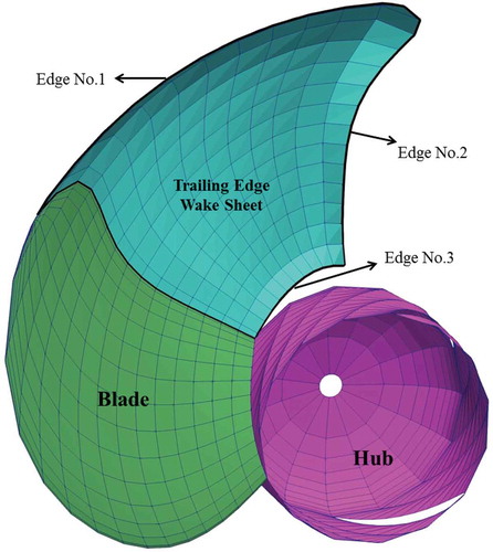
The first item in Equation (9)(9) $\overrightarrow{{\nu }_m}=\frac{1}{4\pi }\text{mathop {}\sum \text{^ }limits\_}{S}_B\text{ {}\int \text{^ ^}}(\overrightarrow{n}.\overrightarrow{q})\overrightarrow{\frac{r}{r^3}}dS+\frac{1}{4\pi }\text{mathop {}\sum \text{^ }limits\_}{S}_B\text{ {}\int \text{^ ^}}\varphi \frac{\overrightarrow{dl}\times \overrightarrow{r}}{r^3}dS+\text{ mathop {}\sum \text{^ }limits\_}{S}_B\text{ {}\int \text{^ ^}}\mu \frac{\overrightarrow{dl}\times \overrightarrow{r}}{r^3}dS$(9) is the surface integral term with regular kernel for free wake points. The second and third terms are dipoles line integral over the boundary lines of each wake. These lines are schematically shown in Figure 2 for a blade wake sheet. It should be mentioned that these integrals represent the Biot-Savart formula for calculating the induced velocity for the singular vortex line (Katz & Plotkin, 1991).

Figure 2. Integration over boundary lines.

2.3. Hydrodynamic forces and moments

After calculating the potential velocity field, it is possible to compute the pressure by applying the unsteady Bernoulli equation over each panel. The unsteady form of Bernoulli equation is written as follows (Najafi & Abbaspoor, 2017):

(10) $\frac{P-P_{\mathrm{\infty }}}{\rho }=-\frac{d\varphi }{dt}-\frac{1}{2}{\left|\overrightarrow{\mathrm{\nabla }}\varphi -{\overrightarrow{\mathrm{\nabla }}}_{rel}\right|}^2+\frac{1}{2}{\left|{\overrightarrow{\mathrm{\nabla }}}_{rel}\right|}^2,$(10)

where ${ }_{rel}$ is the relative velocity of each panel and $\varphi$ is the surface gradient of the velocity potential. The relative velocity can be computed as follows:

(11) $V_{rel}=\overrightarrow{V}\left(t\right)\to \overrightarrow{\mathrm{\Omega }}\left(t\right)\times \overrightarrow{r}.$(11)

In almost all the CFD methods, the hydrodynamic force and moment are calculated by integrating the pressure (normal stress) and friction (shear stress) forces over the body. Since boundary element method is based on the assumption that fluid in inviscid, an artificial method should be applied to estimate the friction force. In this paper, an experimental drag coefficient is utilized, which has been proposed by Blevins (Politis, 2005) for a smooth flat plate:

(12) $\overrightarrow{D}=0.5\rho C_D\overrightarrow{V}{ }_{tot}\left|{\overrightarrow{V}}_{tot}\right|,\overrightarrow{V}{ }_{tot}=\overrightarrow{V}{ }_{ref}+\overrightarrow{V}\varphi$(12)

(13) $C_D=\frac{0.0986}{{\left(logRe-1.22\right)}^2}$(13)

As observed in this formula, the local friction coefficient,${\mathrm{C}}_{\mathrm{D}}$, is very dependent on the Reynolds number. This formula is very common to virtually calculate viscous effects in potential solvers such as BEM (Politis, 2004; Najafi & Abbaspoor, 2017). Reynolds number corresponding the propeller is defined by the following formula (Ochi et al., 2009):

(14) $Re=\frac{C_{0.7R}\sqrt{V_a^2+{\left(0.7\pi nD\right)}^2}}{\nu }$(14)

where C0.7 R is the chord length at 70% position of the propeller radius, $V_a$ is the inflow velocity of the propeller, n is the revolution rate, D is the propeller diameter and $\nu$ is the kinematic viscosity.

Therefore, the hydrodynamic forces and moment can be calculated using

(15) $\overrightarrow{F}=\text{ mathop {}\int \text{^ }limits\_}S\left(p\overrightarrow{n}+\overrightarrow{D}\right)dS$(15)

(16) $\overrightarrow{M}=\text{ mathop {}\int \text{^ }limits\_}S\overrightarrow{r}\times \left(p\overrightarrow{n}+\overrightarrow{D}\right)dS$(16)

2.4. Developed code

In the developed code, the data structure is designed in such a way that each lifting body is defined separately with separated wake sheet. This implies that for a three-blade propeller, three lifting bodies are defined (Figure 3).

Figure 3. Lifting bodies in data structure.

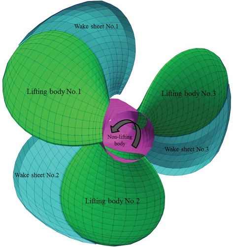
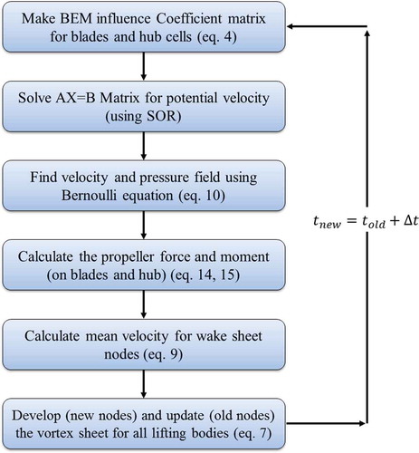
It is therefore necessary that the proposed method be repeated for all lifting bodies at each step before advancing to the next time step. For better understanding of the algorithm, a flowchart is presented in Figure 4.

Figure 4. Applied algorithm in the developed solver.

3. Validation of the results

3.1. Marine propeller DTMB4119

As pointed out earlier, the DTMB4119 marine propeller is utilized for validation of the results of the proposed numerical model, since extensive studies have been carried out on this standard propeller. Jessup (Jessup, 1989) experimentally studied the DTMB4119 propeller and published his findings. In 1982 (Jessup, 1989) and 1990 (Jessup, 1982), he measured unsteady blade force and pressure distribution of the well-known propellers (DTMB 4119, DTMB 4679) in axial and oblique flow. Table 1 shows the results of an open water test for DTMB4119.

Table 1. Open water test for DTMB4119

$J$	$K_T$	$10K_Q$	$\eta \left(\mathrm{\%}\right)$
0.5	0.28	0.46	48.44
0.7	0.21	0.36	63.44
0.833 (design point)	0.15	0.28	71.02
0.9	0.13	0.24	74.6
1.0	0.08	0.18	66.31
1.1	0.03	0.11	47.75

In this table,$j$,$K_T$, $K_Q$ and $\eta$ are advance ratio (coefficient), thrust coefficient, torque coefficient and efficiency, respectively. These parameters are defined as follows:

(17) $J=\frac{V_a}{nD}$(17)

(18) $K_T=\frac{T}{\rho n^2{D}^4}$(18)

(19) $K_Q=\frac{T}{\rho n^2{D}^5}$(19)

(20) $\eta =\frac{J}{2\pi }\frac{K_T}{K_Q}$(20)

where $\mathrm{n}$and $\mathrm{D}$ are the rotational speed and diameter of the propeller, respectively. $V_a$ is freestream fluid velocity. As illustrated in Table 1, $J=0.833$ is the design point for the DTMB4119 propeller. In the current study, quadratic surface panels are used to discretize the desired geometry. Figure 5 shows the discretized propeller.

Figure 5. Discretized geometry of DTMB 4119 propeller.

In order to adopt an optimum mesh size for the simulations, it is necessary to conduct a mesh independency study. For this purpose, five different mesh sizes are investigated. Due to complexity of the flow around the leading and trailing edges of the propeller, cosine spacing is used with uniform increments. As a result, mesh density increases around edges of the blades. The hub mesh size is considered appropriate to the blade mesh size such that there is minimum difference between them. The propeller diameter and free velocity are assumed to be $\mathrm{D}=1.0\mathrm{m}$ and $\mathrm{V}=1\frac{\mathrm{m}}{\mathrm{s}}$, respectively. Politis (2004) conducted a study on time stepping method. As adopted in this paper, the time step ($\delta \mathrm{t}$) is selected according to step angle of 8 degrees (Politis, 2004). This implies that at each time step, the propeller rotates 8 degrees. The results of the mesh study are obtained at design advanced ratio of $J=0.833$ and are illustrated in Table 2. All the simulations are performed on a 2.5GH corei5 personal laptop.

Table 2. Results of the mesh study at$\mathrm{J}=0.833$

Mesh no.	No. of panels in blades	No. of panels in hub	Computational time (sec)	Thrust coefficient $K_T$	Error (%)
1	300	70	1655	0.167	11.10
2	900	120	3730	0.158	5.50
3	1800	390	10490	0.151	0.70
4	3000	450	22116	0.149	0.38
5	4500	510	43759	0.151	0.35

Figure 6 shows the convergence rate of the thrust at $J=0.833$ for different mesh size. As shown in this figure, all the targeted simulations are performed until the propeller generated force becomes stable. In this case, it is quite clear that 1.4 sec of simulation time is sufficient.

Figure 6. Convergence rate of thrust at $\mathrm{J}=0.833$.

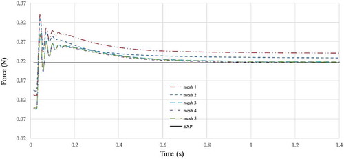
Based on the presented results in Figure 6, it is obvious that the mesh size no. 3 is proper enough to be chosen for the targeted simulations in the current study. This mesh is composed of 20 panels in spanwise direction and 15 panels in chordwise direction of each blade (Figure 5).

The rollup patterns of the trailing vortex sheet for the considered propeller are displayed in Figure 7. (The mesh size for this simulation in the present work is no. 2.)

Figure 7. Rollup pattern for propeller DTMB4119 at $\mathrm{J}=0.833$. (Left: Propeller angle = 180^O, Right: Propeller angle = 360^O) (Top: Politis (Politis, 2004), Bottom: Present work).

The performance chart of examined DTMB4119 propeller is plotted in Figure 8. As shown in Figure 8, the thrust coefficient has good accuracy, while the computed torque coefficient displays slightly different result compared with experimental data. This discrepancy can be attributed to the inviscid nature of BEM method.

Figure 8. Performance chart for DTMB4119.

To verify the accuracy of the numerical results in more details, one could compare the pressure coefficient on blade sections with experimental data (Jessup, 1982). Pressure coefficient may be easily calculated using the undisturbed velocity as in

(21) ${\mathrm{C}}_{\mathrm{P}}=\frac{P-P_{\mathrm{\infty }}}{0.5\rho \left|\hspace{0.17em}\right|}$(21)

Jessup (1982) reported the pressure coefficient along the chord wise section of the DTMB4119 propeller at three radial sections ($\mathrm{r}/\mathrm{R}=0.3,0.7,0.9$). Figure 9 shows the comparison of the numerical results with experimental data (Jessup, 1982). For better visualization and in order to avoid chaos, the results of three mesh sizes (no. 2, 3 and 5) are shown.

Figure 9. Pressure coefficient distribution along chord wise section of DTMB4119 at $J=0.833$.

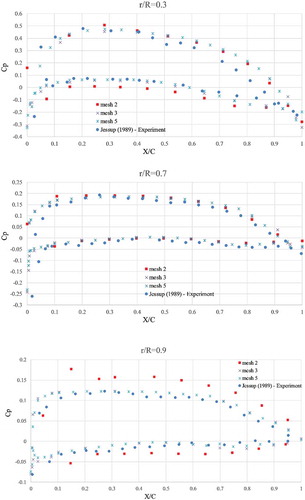
As evident in Figure 9, the obtained results at $r/R=0.7$ shows good agreement with the experimental data. However, there are relatively poor matching at$r/R=0.3,0.9$ ratios. This is due to the complex 3D viscous nature of the flow in these regions which cannot be precisely simulated by the inviscid numerical models such as BEM (Politis, 2011). Once again it can be concluded from these results that mesh size no. 3 is fine enough to capture all hydrodynamic phenomena.

3.2. Marine propeller KP505

In order to examine the ability of the proposed method for modeling the wake pattern, the KP505 propeller is simulated. KP505 is a five-blade marine propeller which is designed for the KRISO container ship (KCS). Table 3 shows main particulars of the KP505 propeller.

Table 3. Main particulars of the KP505 propeller

Number of blades	5
Propeller diameter ($m$)	0.15
Boss ratio	0.18
Pitch ratio at 0.7 R	0.997
Expanded blade area ($m^2$)	0.8

Figure 10 shows the mesh size of the propeller which is created as described in the previous section. The designed advance ratio of KP505 is $J=0.7$. The hydrodynamic performance of the propeller was calculated, using the suggested method.

Figure 11 shows the hydrodynamic performance chart of KP505 which is compared with the experimental data (Fujisawa et al., 2000). As evident in Figure 10 the simulated results display good accuracy of the obtained thrust and torque coefficients, especially at high advance ratios. This is due to BEM high performance, which can be used in the preliminary design purposes.

Figure 10. Discretized KP505 propeller (3015 cells).

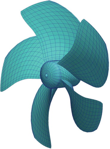
Figure 11. Performance chart of the KP505 propeller.

As pointed out earlier, KP505 is a five-blade propeller which implies that five wake sheet rollup patterns should be simulated behind the propeller. In generating the wake sheet of each propeller, the influence of other blades should be taken into consideration. Figure 12 shows the rollup pattern of the wake sheets in three different time steps at designed advance ratios.

Figure 12. Rollup pattern for propeller KP505 at $J=0.7$. (Left: Propeller angle = 180^O, Middle: Propeller angle = 360^O, Right: Propeller angle = 720^O).

3.3. Skewed B-Series controllable pitch propeller

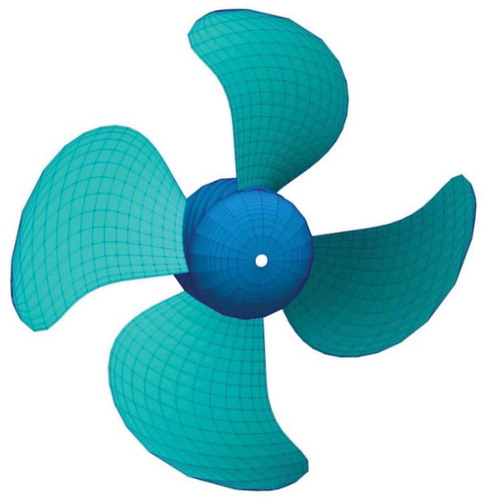
In this section, the hydrodynamic performance parameters of an applied controllable pitch (CP) propeller are investigated, as a validation test case. After validation, simulations for different hub diameters are performed. This propeller is designed for a Research Vessel (RV). The main particulars of this propeller as well as the cross-section parameters of each blade are presented in Tables 4 and 5 respectively.

Table 4. Main particulars of the RV propeller

Number of blades	4
Propeller diameter ($m$)	2.1
Hub Diameter (m)	0.56
Expanded blade area ($m^2$)	1.95
Mean pitch ($mm$)	1691.1
Design $J=V/nD$	0.623

Table 5. Cross section parameters of the RV propeller blade

$\frac{r}{R}$	$\frac{c}{D}$	$\frac{P}{D}$	$Skew{(}^o)$	$\frac{rk}{D}$	tmax/c
0.3	0.2011	0.7905	−5.6000	0.0050	0.0261
0.4	0.2553	0.8318	−8.5400	0.0047	0.0222
0.5	0.3033	0.8473	−9.7900	0.0027	0.0184
0.6	0.3413	0.8490	−9.2000	−0.0013	0.0149
0.7	0.3662	0.8390	−5.9800	−0.0073	0.0117
0.8	0.3750	0.8148	0.0000	−0.0154	0.0088
0.9	0.3281	0.7479	8.7400	−0.0254	0.0060
1	0.0188	0.6040	20.2300	−0.0375	0.0032

As shown in Table 4, the propeller is designed for advanced ratio of $J=0.623$. The available results of the open water test for this propeller are presented in Table 6.

Table 6. The results of the open water test for the RV propeller

$J$	$K_T$	$10K_Q$	$\eta \left(\mathrm{\%}\right)$
0.2	0.3133	0.3818	0.2612
0.3	0.2795	0.3468	0.3848
0.4	0.2425	0.3079	0.5014
0.5	0.2025	0.2649	0.6083
0.6	0.1601	0.2179	0.7016
0.7	0.1155	0.1667	0.7723
0.8	0.0693	0.1113	0.7935
0.9	0.0219	0.0516	0.6073

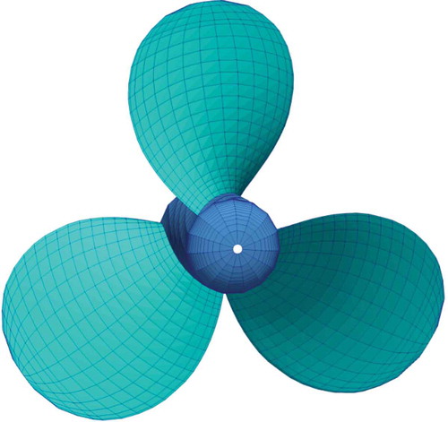
The discretized propeller in this simulation consists of 2980 cells (600 cells for each blade and 580 cells in hub) which is displayed in Figure 13.

Figure 13. Discretized RV propeller (2980 cells).

All the intended simulations are performed at different advanced ratios for three propeller revolutions. The numerical results in the form of (${\mathrm{K}}_{\mathrm{T}},{\mathrm{K}}_{\mathrm{Q}},\eta$) are compared with those of the open water test in Figure 14. As pointed out earlier, the time step is set to 8 degree of propeller rotation and the simulations are performed until the thrust force becomes steady. Because of different propeller rotational speeds at each advance ratio, the overall simulation time is different, and it is concluded that hydrodynamic thrust becomes steady at nearly five propeller revolution.

Figure 14. Performance chart for the RV propeller.

Figure 14 indicates that thrust coefficient is predicted with good accuracy (less than 10% in design advance ratios) which is acceptable for design purposes, while the torque coefficient accuracy is relatively low (below 16% in design advance ratios) and this is again due to inviscid nature of the BEM approach. Estimated errors for the thrust and torque coefficients are shown with more details in Table 7.

Table 7. Numerical results and thrust/coefficient errors, compared to the open water test data

$J$	$K_T$	$10K_Q$	$errorof{K}_T\left(\mathrm{\%}\right)$	$errorof{K}_Q\left(\mathrm{\%}\right)$
0.2	0.361	0.468	15.18	22.61
0.3	0.320	0.420	14.32	21.17
0.4	0.269	0.355	10.81	15.41
0.5	0.220	0.302	8.66	14.10
0.623 (design)	0.161	0.231	7.21	11.44
0.7	0.122	0.185	5.35	10.73
0.8	0.073	0.120	4.74	7.51
0.9	0.023	0.055	4.56	6.80

The rollup pattern of the propeller is illustrated in Figure 15. With regard to the computational time, it should be mentioned that each case is simulated in about 3 hours (11,015 seconds) on a 2.5 GHz Corei5 personal computer.

Figure 15. Rollup pattern for RV propeller at 720 degree of revolution at $\mathrm{J}=0.623$.

4. Results and discussion

After the validation parts, the proposed solver is used to analyze the effect of hub diameter on the propeller hydrodynamic behavior. For this purpose, the RV CP propeller was selected. Ten different hub diameters are chosen from minimum 0.42 m up to about 1.0 m. The blade geometry is the same in all cases, while the hub diameter is different. The hydrodynamic performance of each propeller is calculated using the proposed BEM solver. Figure 16 shows some discretized CP propellers.

Figure 16. Discretized CP propeller of research vessel with different hub diameter.

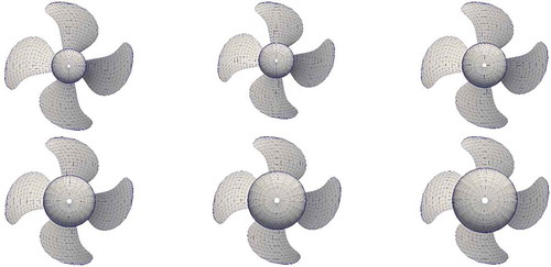
Table 8 shows the hydrodynamic performance of propeller with different (non-dimensional) hub/propeller diameter.

Table 8. Hydrodynamic performance of the propeller at different hub diameters

$hubdiameter\left(m\right)$	Hub/propeller diameter	$K_T$	$10K_Q$	$\eta \left(\mathrm{\%}\right)$
0.420	0.2	0.1676	0.2395	0.6938
0.462	0.22	0.1661	0.2376	0.6931
0.525	0.25	0.1633	0.2338	0.6923
0.567	0.27	0.1608	0.2307	0.6913
0.630	0.3	0.1564	0.2253	0.6882
0.672	0.32	0.1529	0.2207	0.6868
0.735	0.35	0.1470	0.2127	0.6854
0.777	0.37	0.1427	0.2068	0.6843
0.840	0.4	0.1357	0.1969	0.6831
0.945	0.45	0.1219	0.1769	0.6833

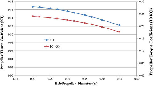
Figure 17 shows the thrust and torque coefficients in this parametric situation. As expected, the thrust decreases by increasing the hub diameter. This is an obvious phenomenon, since a propeller with shorter blades (bigger hub) generates less thrust. On the other hand, the hub diameter has contra-effect on torque, too. For better visualization, consider a smooth cylindrical hub without any propeller. In that case, the torque is minimized. This is due to the fact that blades (with non-zero pitch) would tolerate more torque than smooth spherical hub.

However, Figure 17 does not offer a practical way to select hub diameter. Therefore, it is better to seek the hub diameter in a curve other that $K_T,and{K}_Q$. Propeller efficiency is a better choice for this purpose (Figure 18).

Figure 17. Thrust and torque coefficients versus hub diameters.

Efficiency diagram is another main parameter in hydrodynamic performance of a propeller which should judiciously be taken into consideration. Figure 18 shows this diagram versus hub/propeller diameter (calculated by Equation (18)(18) $K_T=\frac{T}{\rho n^2{D}^4}$(18) ).

As evident in this figure, as hub diameter increases, the propeller efficiency gradually decreases, but there is something important to be noted in this process, which is the trend of the plot, or in other words, its slope at different points. It is noticed that curve concavity is initially tends downward and then as hub diameter increases, concavity changes to upward. With an increase in hub diameter until point no. 1, efficiency reduction is relatively small, but after that, a drastic reduction is observed. Therefore, the designer of the propeller pitch variation mechanism should select a hub diameter less than that of point no. 1 (hub/propeller diameter = 0.27) for the design purposes. Otherwise, it is suggested that propeller’s blades geometry and even their numbers should be reviewed and rethought.

Figure 18. Propeller efficiency at different hub diameters.

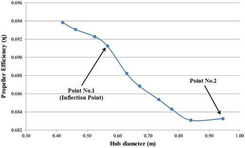
Although there is a little surge in efficiency at point no. 2 (compared to the previous point), but certainly it cannot be taken as a suggestion point for the hub diameter, because the efficiency is rather low.

Typically, the CPP hub has a diameter in the range of 0.24D to 0.32D (D is the propeller diameter), but for some applications this may rise to as high as 0.4D or even 0.5D (Carlton, 2007). Since BEM method was shown to be a rather fast and efficient method to simulate the propeller hydrodynamics, Figure 18 could be referenced as a guideline for the designers to select hub diameter with better estimations (especially in preliminary states). There are also two main mechanisms for propeller pitch changing: (1) pull-push rod system¹ and (2) hub piston system (Carlton, 2007). The hub piston systems are relatively easier to design but require bigger hub bossing. Figure 17 could also help designers to select the mechanism with better sight.

In order to show the effect of hub diameter in more details, the pressure coefficient along the chord wise section of the blade is plotted at $\frac{r}{R}=0.7$ for all cases in Figure 19.

It can be seen that pressure difference between upper and lower face of the propeller section reduces by an increase in the hub diameter. As this difference is the main factor for blade section to produce thrust, it is the main reason behind the propeller with larger hub diameter producing less thrust. For better investigation, the pressure coefficient for the hub/propeller diameter = 0.2 and 0.45 is compared on the same plot in Figure 20.

Figure 19. The pressure coefficient along the chord wise section of the blade.

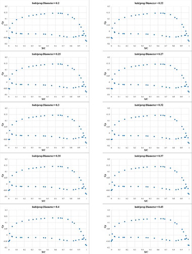
Figure 20. The pressure coefficient comparison for the hub/propeller diameter = 0.2 and 0.45.

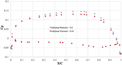
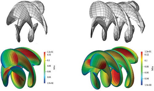
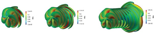
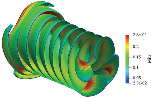
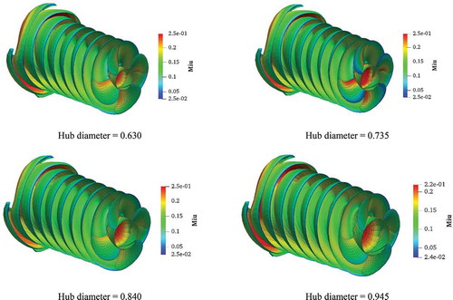
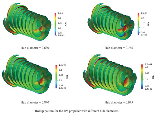
Figure 20 reveals that the reduction in pressure coefficient is mainly related to the upper (the face which is in front of the free stream velocity) cross-sectional of the propeller. The rollup wake sheet for the RV propeller at different hub diameters are shown in Figure 21. (Each propeller rotated 720 degrees.)

Figure 21. Rollup pattern for the RV propeller with different hub diameters.

5. Conclusions

A three-dimensional unsteady boundary element method is presented to simulate flow around marine propeller. The BEM approach is chosen over RANS based methods for its higher capability in terms of computational time, easy implementation, and relatively good accuracy in simulating the lifting bodies. The Time Stepping Method (TSM) is used to simulate the wake sheet rollup at each time step. This wake sheet is generated behind the trailing edges of the blade which helps satisfy the $\mathrm{\Gamma }=0$ in the flow field. On the other hand, for better accuracy, the propeller is composed of blades (lifting bodies) and hub (non-lifting body) in a way that the effect of hub can be captured in each simulation. Investigating the effect of hub diameter on hydrodynamic performance of CPPs was the motivation of this paper for developing such a solver.

The proposed solver is validated by three experimental test cases. These cases include DTMB4119, KP505 standard marine propellers, and a high skew B-series CP propeller. Relatively good agreement is displayed in all cases. Subsequently, the proposed numerical model is used to perform a series of parametrical simulations to study the effect of hub diameter on a high skew CPP efficiency. Based on the obtained results, one may conclude that the efficiency curve of the propeller can be applied to establish a balance between the hub diameter and propeller performance. It is shown that this curve can be referred as a guideline for selecting a non-dimensional hub diameter or choosing the pitch mechanism. In this case, the hub/propeller diameter of 0.27 is presented as a proper diameter which not only provides a better housing for the CPP mechanism, but also reduces the propeller efficiency with reasonable value. This algorithm can be applied for any similar test cases in preliminary and basic design stages.

Nomenclature

$\varphi \left(\mathrm{x},\mathrm{t}\right)$	=	Velocity potential
r	=	Position vector between source point and field point
$\mu$	=	Doublet intensity of wake panel
$\left(t\right)$	=	Linear velocity
$\overrightarrow{V_{rel}}$	=	Relative velocity
$Re$	=	Reynolds number
$C_D$	=	Drag coefficient
$D$	=	Propeller diameter
$J$	=	Advanced coefficient
$K_Q$	=	Torque coefficient
$F$	=	Hydrodynamic force
$\rho$	=	Fluid density
$\nu$	=	Fluid kinematic viscosity
$\overrightarrow{{\nu }_m}$	=	Mean perturbation velocity
n	=	Unit normal vector of panel pointing outward of the body
$\overrightarrow{X_i}$	=	Wake sheet node position
$Q\to \left(t\right)$	=	Angular velocity
$P$	=	Pressure on panel
$P_{\mathrm{\infty }}$	=	Far field pressure
$C_P$	=	Pressure coefficient
$n$	=	Propeller rotational speed
$V_a$	=	Freestream fluid velocity
$K_T$	=	Thrust coefficient
$M$	=	Hydrodynamic moment
$C_{0.7R}$	=	Chord length at 70% position of propeller radius

Cover image

Source: Author.

Acknowledgements

This research received no specific grant from any funding agency in the public, commercial, or not-for profit sectors and there is no conflict of interest.

Additional information

Funding

The authors received no direct funding for this research.

Notes on contributors

Parviz Ghadimi

Professor Parviz Ghadimi received his Ph.D. in Mechanical Engineering in 1994 from Duke University, USA. He served one year as a Research Assistant Professor in Mech. Eng. Dept. and six years as a Visiting Assistant Professor in Mathematics Dept. at Duke. He then joined Dept. of Maritime Engineering at Amirkabir University of Technology, Iran, in Fall 2005. He is currently a Full Professor of Hydromechanics at that department. His main research interests include hydrodynamics, hydro-acoustics, thermo-hydrodynamics, and CFD, and he has authored over one hundred scientific papers as well as six books in these fields. The current topic is the result of a particular research in his hydrodynamic group which focuses on simulation of a high-skew Controllable Pitch Propeller with different hub diameters.

Notes

1. This mechanism is usually used in the propellers which require lower power to change the pitch

References

- Benek, J. A., Steger, J. L., & Dougherty, F. C. (1983). A flexible grid embedding technique with application to the Euler equations. AIAA, 6th Computational Fluid Dynamics Conference; AIAA Paper No. 1983-1944.
- Bennaya, M., Gong, J., Hegaze, M. M., & Zhang, W. (2013). Numerical simulation of marine propeller hydrodynamic performance in uniform inflow with different turbulence models. Applied Mechanics and Materials, 389, 1019–26. https://doi.org/10.4028/www.scientific.net/AMM.389.1019
- Brizzolara, S., Villa, D., & Gaggero, S. (2008). A systematic comparison between RANS and panel method for propeller analysis. Proceeding of the 8th international conference on hydrodynamics, Nantes, 30 Sep - 3 Oct.
- Carlton, J. S. (2007). Marine propellers and propulsion (second ed.). Butterworth-Heinemann.
- Dubbioso, G., Muscari, R., & Mascio, A. D. (2013). Analysis of the performances of a marine propeller operating in oblique flow. Computers & Fluids, 75, 86–102. https://doi.org/10.1016/j.compfluid.2013.01.017
- Felice, F. D., Felli, M., Liefvendahl, M., & Svennberg, U. (2009). Numerical and experimental analysis of the wake behavior of a generic submarine propeller, First International Sympsium of Marine Propulsor, Trondheim, Norway.
- Fujisawa, J., Ukon, Y., Kume, K., & Takeshi, H. (2000). Local velocity field measurements around the KCS model (SRI M.S.No.631) in the SRI 400 m towing tank. ShipPerform. Div. Rep. No., 00–003-02.
- Gaafary, M. M., EL-Kilani, H. S., & Moustafa, M. M. (2011). Optimum design of B-series marine propellers. Alexandria Engineering Journal, 50(1), 13–18. https://doi.org/10.1016/j.aej.2011.01.001
- Gaggero, S., Dubbioso, G., Villa, D., Muscari, R., & Viviani, M. (2019). Propeller modeling approaches for off–design operative conditions. Ocean Engineering, 178, 283–305. https://doi.org/10.1016/j.oceaneng.2019.02.069
- Gaggero, S., Villa, D., & Brizzolara, S. (2010). RANS and PANEL method for unsteady flow propeller analysis. 9th International Conference on Hydrodynamics, October 11-15, Shanghai, China.
- Greco, L., Muscari, R., Testa, C., & Di Mascio, A. (2014). Marine propellers performance and flow-field prediction by a free-wake panel method. Journal of Hydrodynamics, 26(5), 780–795. https://doi.org/10.1016/S1001-6058(14)60087-1
- Henshaw, W. D., & Schwendeman, D. W. (2006). Moving overlapping grids with adaptive mesh refinement for high-speed reactive and non-reactive flow. Journal of Computational Physics, 216(2), 744–779. https://doi.org/10.1016/j.jcp.2006.01.005
- Hess, J. L. (1972). Calculation of potential flow around arbitrary three dimensional lifting bodies, Report no. MDC J5679-01, McDonnell Douglas Corporation.
- Hess, J. L., & Smith, A. M. O. (1962). Calculation of non-lifting potential flow about arbitrary 3-D bodies. Douglas Aircraft Report E.S. 40622.
- Hess, J. L., & Valarezo, W. O. (1985). Calculation of steady flow around propellers by means of a surface panel method. In: Proceedings of the 23rd Aerospace Sciences Meeting, AIAA, Reno, Nev.
- Jessup, S. (1982). Measurements of the pressure distribution on two model propellers, DTNSRDC82/035 Technical Report.
- Jessup, S. D. (1989). An experimental investigation of viscous effects of propeller blade flow (PhD Thesis), The Catholic University of America.
- Katz, J., & Plotkin, A. (1991). Low-speed aerodynamics. McGraw-Hill.
- Lim, -S.-S., Kim, T.-W., Lee, D.-M., Kang, C.-G., & Kim, S.-Y. (2014). Parametric study of propeller boss cap fins for container ships. International Journal of Naval Architecture and Ocean Engineering, 6(2), 187–205. https://doi.org/10.2478/IJNAOE-2013-0172
- Meakin, R. L., & Suhs, N. E. (1989). Unsteady aerodynamic simulation of multiple bodies in relative motion. AIAA, 9th Computational Fluid Dynamics Conference; AIAA Paper No. 1989-1996.
- Miglianti, L., Cipollini, F., Oneto, L., Tani, G., Gaggero, S., Coraddu, A., & Viviani, M. (2020). Predicting the cavitating marine propeller noise at design stage: A deep learning based approach. Ocean Engineering, 209, 107481. https://doi.org/10.1016/j.oceaneng.2020.107481
- Najafi, S., & Abbaspoor, M. (2017). Numerical investigation of flow pattern and hydrodynamic forces of submerged marine propellers using unsteady boundary element method. Engineering for the Maritime Environment, Published online, 233(1), 1–13. https://doi.org/10.1177/1475090217717174
- Najafi, S., & Abbaspour, M. (2017). Numerical study of propulsion performance in swimming fish using boundary element method. Journal of the Brazilian Society of Mechanical Sciences and Engineering, 39(2), 443–455. https://doi.org/10.1007/s40430-016-0613-8
- Ochi, F., Fujisawa, T., Ohmori, T., & Kawamura, T. (June 2009). Simulation of propeller hub vortex flow. First international symposium on marine propulsors, Trondheim, Norway.
- Politis, G. K. (2004). Simulation of unsteady motion of a propeller in a fluid including free wake modeling. Engineering Analysis with Boundary Elements, 28(6), 633–653. https://doi.org/10.1016/j.enganabound.2003.10.004
- Politis, G. K. (2005). unsteady rollup modeling for wake adapted propellers using a time stepping method. Journal of Ship Research, 49(3), 216–231.
- Politis, G. K. (2011). Application of a BEM time stepping algorithm in understanding complex unsteady propulsion hydrodynamic phenomena. Ocean Engineering, 38(4), 699–711. https://doi.org/10.1016/j.oceaneng.2011.01.001
- Rahman, A., Ullah, M. R., & Karim, M. M. (2017). Marine propeller design method based on lifting line theory and lifting surface correction factors. Procedia Engineering, 194(174), 256. https://doi.org/10.1016/j.proeng.2017.08.132
- Shamsi, R., Ghassemi, H., Molyneux, D., & Liu, P. (2014). Numerical hydrodynamic evaluation of propeller (with hub taper) and podded drive in azimuthing conditions. Ocean Engineering, 76, 121–135. https://doi.org/10.1016/j.oceaneng.2013.10.009
- Song, B.-W., Wang, Y.-J., & Tian, W.-L. (2015). Open water performance comparison between hub-type and hubless rim driven thrusters based on CFD method. Ocean Engineering, 103, 55–63. https://doi.org/10.1016/j.oceaneng.2015.04.074
- Wang, L.-Z., Guo, C.-Y., Su, Y.-M., & Wu, T.-C. (2018). a numerical study on the correlation between the evolution of propeller trailing vortex wake and skew of propellers. International Journal of Naval Architecture and Ocean Engineering, 10(2), 212–224. https://doi.org/10.1016/j.ijnaoe.2017.07.001
- Zhu, Q., Wolfgang, M. J., YUE, D. K. P., & Triantafyllou, M. S. (2002). Three-dimensional flow structures and vorticity control in fish-like swimming. Journal of Fluid Mechanics, 468, 1–28. https://doi.org/10.1017/S002211200200143X