The Fractional Order Generalization of HP Memristor Based Chaotic Circuit with Dimensional Consistency

Abstract

For studying the practical memristor-based chaotic circuit with fractional-order dynamic and asserting the importance of dimensional consistency awareness, the dimensional consistency aware fractional-order generalization of a Hewlett Packard (HP) memristor-based chaotic circuit with the physical meaning of fractional time component assigned has been proposed in this work. The simplest chaotic circuit based on such practical memristor has been chosen as the candidate circuit. A novel window function dedicated to HP memristor with fractional-order dynamic i.e. fractional-order HP memristor has been adopted for modelling the boundary effect. For the dynamical analysis, the revisited version of Jumarie’s modified Riemann–Liouville fractional derivative and nonlinear transformation has been used. The generalized circuit which has been found to be the simplest fractional-order HP memristor-based chaotic circuit displays a chaotic behavior with significant differences from those of its conventional integer-order prototype and its dimensional consistency ignored counterpart; thus, the importance of dimensional consistency awareness is asserted. The realization of the generalized circuit by using the fractional-order elements is indicated. The circuit emulator has also been presented.

Keywords:

• chaotic circuit
• HP memristor
• dimensional consistency
• fractional order
• fractional time component

PUBLIC INTEREST STATEMENT

In 2008, the memristor has been physically realized by researchers in Hewlett Packard (HP) labs after being postulated by L. Chua in 1971 and has been utilized in various circuits. According to the rise of fractional-order circuits, an HP memristor-based chaotic circuit with multiple memristors has been generalized to fractional order. However, the dimensional consistency which significantly affects the dynamic of generalized chaotic circuit has been ignored. In addition, there exists a simpler single HP memristor-based chaotic circuit. Therefore, a dimensional consistency aware fractional-order generalization of such simpler circuit has been performed in this work with the physical meaning of fractional time component given. Our generalized circuit is dimensional consistent yet simpler than the previous one. This work is beneficial to the analysis and design of chaotic circuits, fractional-order circuits, HP memristor-based circuits, nonlinear circuits, etc.

1. Introduction

Long before the invention of a novel electronic device like a wearable robot controller (Chu et al., 2020), the state of the art fourth fundamental electrical circuit element namely memristor has been postulated by Chua (Chua, 1971). For decades later yet before many recent research studies, e.g., (Omidi et al., 2017), (Ahmadi & Azhari, 2018), and (Shotorbani & Saghai, 2018) etc., have been proposed, the memristor has been physically realized by a research group in Hewlett Packard (HP) labs in 2008. The realized memristor which is often referred to as the HP memristor is based on a nanoscale TiO₂ technology (Strukov et al., 2008) and has been utilized in various circuits including the chaotic circuits. For examples, the autonomous circuit with two memristors connected in an antiparallel fashioned has been proposed in Buscarino et al., (2012) where a simpler single memristor-based circuit has been later proposed by Guang-Yi et. al. (Guang-Yi et al., 2013). A non-autonomous circuit has been proposed in G. Wang et al., (2015) and a circuit which is both autonomous and employs fewer elements than the previous ones including its predecessor (Wang, Sun, Jin, Mo, Song, Dong et al., 2018a, May); thus, it is the simplest HP memristor-based chaotic circuit has been proposed by Wang et. al. (Wang, Sun, Jin, Mo, song, Dong et al., 2018a). Apart from being the simplest one, the correct assumption on HP memristor has also been assumed in its designing process unlike the previous non-autonomous circuit which it has been incorrectly assumed in (G. Wang et al., 2015) that the HP memristor is locally active despite that this device is actually passive (Strukov et al., 2008) due to the boundary effect.

According to the rise of fractional-order circuits, on the other hand, the fractional-order generalization of chaotic circuits has been performed in many previous works where the simplest Chua’s chaotic circuit which operates in a voltage mode (Muthuswamy & Chua, 2010) has been considered in Cafagna & Grassi, (2012). The antiparallel fashioned connected HP memristor-based chaotic circuit proposed by Buscarino et al. has been generalized by Deng et al. (Deng & Wang, 2013). The simplest Chua’s circuit with fourth degree nonlinearity has been studied by Teng et.al. (Teng et al., 2014). The bifurcation analysis and stabilization of fractional-order Chua’s circuit have been, respectively, performed in Abdelouahab & Lozi, (2015) and Yang et al., (2016). A fractional derivative with nonlocal-nonsingular kernel (Atangana & Baleanu, 2016) has been applied by Alkahtani (Alkahtani, 2016). Recently, both simplest Chua’s chaotic circuit and the simplest current mode chaotic circuit proposed by Jin et al. (Jin et al., 2017) have been generalized by Banchuin (Banchuin, 2020). In all of these works but Banchuin, (2020), the dimensional consistency has been ignored. Such dimensional consistency is often cited in many studies on the fractional-order generalization of linear circuit where the classical Caputo’s definition of fractional derivative has been applied in Gómez et al., (2013) and Gómez-Aguilar et al., (2014). A nonsingular kernel fractional derivative (Caputo & Fabrizio, 2015) has been applied in Atangana & Alkahtani, (2015). A nonlocal-nonsingular kernel derivative has been adopted by Gómez‐Aguilar et al. (Gómez‐Aguilar et al., 2017). On the other hand, the conformable fractional derivative (Khalil et al., 2014) has been applied by Martinez et al. (Martinez et al., 2018). For nonlinear circuit, on the other hand, the dimensional consistency has been mentioned only in Banchuin, (2020) which stated that such consistency significantly affects the dynamics of the circuit generalized chaotic circuit. However, the memristors assumed in this previous work are merely the hypothetical ones unlike the HP memristor which is a physically realized device. In addition, the physical meaning of fractional time component has never been assigned in Banchuin, (2020) despite that such meaning is necessary for obtaining a physically meaningful fractional-order generalization because it can be uniquely assigned depending on the circuit under consideration. As an example, it can be the fraction of time constant for an RC circuit (Gómez-Aguilar et al., 2014), (Martinez et al., 2018). For the LC and RLC circuits, the physical meaning of fractional time component can be related to the reciprocal of oscillating frequency for LC and RLC circuits (Gómez et al., 2013), (Gómez-Aguilar et al., 2014) and so on.

Therefore, a novel fractional-order generalization of a memristor-based chaotic circuit with dimensional consistency awareness has been performed in this work. Unlike (Banchuin, 2020), the HP memristor has been assumed and the physical meaning of fractional time component assigned. The simplest HP memristor-based chaotic circuit with correct memristor assumption has been chosen as our candidate circuit. Unlike Wang, Sun, Jin, Mo, Song, Dong et al., (2018a), a novel window function dedicated to the HP memristor with fractional-order dynamics, thus, can be termed the fractional-order HP memristor as stated above, proposed by Shi et al. (Shi et al., 2018) has been adopted for modelling the boundary effect in this work. For dynamical analysis of the generalized circuit, the revisited version of Jumarie’s modified Riemann–Liouville fractional derivative (Atangana & Secer, 2013) and nonlinear transformation (Mahmoud et al., 2017) have been adopted. The simulations have been performed via MATHEMATICA. The Lyapunov exponents and dimensions have also been calculated. As a result, we have found that the generalized circuit displays a chaotic behavior with significant differences from those of its integer-order prototype proposed by Wang et al., and its dimensional consistency ignored counterpart; thus, the importance of dimensional consistency awareness has been asserted. The circuit’s eigenvalues have been solved and used for deriving the chaoticcriteria. In addition, the bifurcation analysis has been performed. As a result, it has been shown that the circuit ceases to be chaotic if at least one of these criteria is violated and the circuit has undergone through a Hopf bifurcation at its equilibrium. The realization of the generalized circuit by using the fractional-order elements is indicated. Compared with the previous fractional-order circuit proposed by Deng et al., our generalized circuit is simpler apart from being dimensional consistent as merely a single fractional-order HP memristor is required. As a result, it has been found to be the simplest fractional-order HP memristor-based chaotic circuit. In addition, the emulator has also been presented.

In the following section, an overview of HP memristor will be given followed by an introduction of the candidate HP memristor-based chaotic circuit in section III. The proposed fractional-order generalization and dynamical analysis will be presented in section IV where the physical meaning of the fractional time component will be assigned and the importance of dimensional consistency awareness will be asserted. The realization of the generalized circuit and the implementation of its emulator will be outlined in section V. Finally, the conclusion will be drawn in section VI.

2. An Overview of HP Memristor

The HP memristor is a nanoscale TiO₂ based device. Its memristance (M(t)) can be given in terms of the minimum and maximum values of M(t) denoted by M_on and M_off and the state variable (x(t)) as (Strukov et al., 2008)

(1) $M(t)=M_{on}x(t)+(1-x(t))M_{off}$(1)

where x(t) which is dimensionless can be given in terms of the memristor’s current (i(t)) and window function (f(x(t), i(t))) as follows:

(2) $\frac{\mathrm{d}}{\mathrm{d}t}x(t)=ki(t)\mathrm{f}(x(t),i(t))$(2)

Noted that k = μM_on/D² where μ and D, respectively, stand for the ion mobility and semiconductor film of thickness. Moreover, M_on ≤ M(t) ≤ M_off as 0 ≤ x(t) ≤ 1 due to the boundary effect of the device which can be modelled by f(x(t), i(t)). Since M_on > 0 (Strukov et al., 2008), M(t) > 0, thus, the HP memristor is passive.

3. The Candidate HP Memristor-Based Chaotic Circuit

Recently, a novel HP memristor-based chaotic circuit has been proposed by Wang et al. (Wang, Sun, et al., 2018a). Compared with the previous circuits mentioned above, this circuit employs minimum number of elements yet autonomous and assumes correct memristor assumption. Thus, it has been chosen. The schematic diagram of this candidate circuit can be depicted in Figure 1. Instead of any f(x(t), i(t)), the truncate function of state variable (trunc(x(t), i(t))) which is given here by (3), has been used for modelling the above-mentioned boundary effects for this circuit. Unfortunately, it can be seen that trunc(x(t), i(t)) lacks both continuity and nonlinearity near x(t) = 0 and x(t) = 1 unlike the formal f(x(t), i(t)).

(3) $\mathrm{t}\mathrm{r}\mathrm{u}\mathrm{n}\mathrm{c}(x(t),i(t))=\{\begin{array}{c}1;\begin{array}{cc}\hspace{0.17em}& 0<x(t)<1\begin{array}{ccccccccc}\hspace{0.17em}& \hspace{0.17em}& \hspace{0.17em}& \hspace{0.17em}& \hspace{0.17em}& \hspace{0.17em}& \hspace{0.17em}& \hspace{0.17em}& \hspace{0.17em}\end{array}\end{array}\\ 0;\begin{array}{cc}\hspace{0.17em}& (x(t)\ge 1\wedge i(t)>0)\vee (x(t)\le 0\wedge i(t)<0)\end{array}\end{array}$(3)

Figure 1. The candidate HP memristor-based chaotic circuit (Wang, Sun, Jin, Mo, Song, Dong et al., 2018a)

4. The Fractional-Order Generalization and Dynamical Analysis

As the first step, the dynamical equations of the candidate HP memristor-based circuit must be reformulated by using the mentioned novel f(x(t), i(t)) instead of trunc(x(t), i(t)). Unlike the previous ones (Joglekar & Wolf, 2009), (Biolek et al., 2009), (Prodromakis et al., 2011), such novel f(x(t), i(t)) is dedicated to the fractional HP memristor as stated above beside being fully scalable with boundary lock issue resolved. According to Shi et al., (2018), this f(x(t), i(t)) and can be given by

(4) $f(x(t),i(t))=1-[a^2(x(t)-\mathrm{u}(-i(t)){)}^2+(1-a^2){]}^p$(4)

where 0 < a ≤ 1 and p > 0. Noted also that u() stands for the unit step function.

As a result, the reformulated dynamical equations of the candidate HP memristor-based chaotic circuit can be obtained as given by (5) which is potentially solvable through a lie algebraic approach (Shang, 2012):

$\frac{\mathrm{d}}{\mathrm{d}t}{i}_1(t)=\frac{1}{L_1}[v_1(t)-(M_{on}x(t)-M_{off}(1-x(t)))i_1(t)]$

(5) $\frac{\mathrm{d}}{\mathrm{d}t}{i}_2(t)=\frac{R}{L_2}{i}_2(t)-\frac{1}{L_2}{v}_1(t)$(5)

$\frac{\mathrm{d}}{\mathrm{d}t}x(t)=k(1-[a^2(x(t)-\mathrm{u}(-i_1(t)){)}^2+(1-a^2){]}^p)i_1(t)$

$\frac{d}{\mathrm{d}t}{v}_1(t)=\frac{1}{C_1}(i_2(t)-i_1(t))$

Secondly, we replaces all conventional derivative terms by fractional derivative ones. In order to achieve the dimensional consistency, the dimensions of conventional and fractional derivative terms must be consistent i.e. both must be given by sec⁻¹. Therefore, the following operation must be used

(6) $\frac{\mathrm{d}}{\mathrm{d}t}\to \frac{1}{{\sigma }^{1-\alpha }}{\mathrm{D}}_t^{\alpha }$(6)

where σ denotes the fractional time component and 0 < α ≤ 1. If we let [T] denote the dimensional formula of time, we have [σ] = [T] and [${\mathrm{D}}_t^{\alpha }$] = [T^−α]. Thus, $\left[\frac{1}{{\sigma }^{1-\alpha }}{\mathrm{D}}_t^{\alpha }\right]$= $\left[\frac{\mathrm{d}}{\mathrm{d}t}\right]$= [T⁻¹] and the dimensional consistency is now achieved. Noted also that the unit of $\frac{1}{{\sigma }^{1-\alpha }}{\mathrm{D}}_t^{\alpha }$which is similar to that of $\frac{\mathrm{d}}{\mathrm{d}t}$ due to the achieved dimensional consistency and is given by sec⁻¹ that is physically measurable always. On the other hand, the unit of ${\mathrm{D}}_t^{\alpha }$ which in turn is given by sec^−α and is physically measurable if and only if α = 1.

After applying (6) to (5), we have

$\frac{1}{{\sigma }^{1-\alpha }}{\mathrm{D}}_t^{\alpha }{i}_1(t)=\frac{1}{L_1}[v_1(t)-(M_{on}x(t)-M_{off}(1-x(t)))i_1(t)]$

(7) $\frac{1}{{\sigma }^{1-\alpha }}{\mathrm{D}}_t^{\alpha }{i}_2(t)=\frac{R}{L_2}{i}_2(t)-\frac{1}{L_2}{v}_1(t)$(7)

$\frac{1}{{\sigma }^{1-\alpha }}{\mathrm{D}}_t^{\alpha }x(t)=k(1-[a^2(x(t)-\mathrm{u}(-i_1(t)){)}^2+(1-a^2){]}^p)i_1(t)$

$\frac{1}{{\sigma }^{1-\alpha }}{\mathrm{D}}_t^{\alpha }{v}_1(t)=\frac{1}{C_1}(i_2(t)-i_1(t))$

After some rearrangement, the following fractional-order dynamical equations can be obtained:

${\mathrm{D}}_t^{\alpha }{i}_1(t)=\frac{1}{L_{1\alpha }}[v_1(t)-(M_{on}x(t)-M_{off}(1-x(t)))i_1(t)]$

(8) ${\mathrm{D}}_t^{\alpha }{i}_2(t)=\frac{R}{L_{2\alpha }}{i}_2(t)-\frac{1}{L_{2\alpha }}{v}_1(t)$(8)

${\mathrm{D}}_t^{\alpha }x(t)=k_{\alpha }(1-[a^2(x(t)-\mathrm{u}(-i_1(t)){)}^2+(1-a^2){]}^p)i_1(t)$

${\mathrm{D}}_t^{\alpha }{v}_1(t)=\frac{1}{C_{1\alpha }}(i_2(t)-i_1(t))$

where$k_{\alpha }=\frac{k}{{\sigma }^{\alpha -1}}$,$C_{1\alpha }=C_1{\sigma }^{\alpha -1}$,$L_{1\alpha }=L_1{\sigma }^{\alpha -1}$and $L_{2\alpha }=L_2{\sigma }^{\alpha -1}$.

Since σ can be assigned with a unique physical meaning depending on the circuit under consideration as stated above, the next step is the assignment of such meaning. Therefore, we let our σ be physically the fraction of reciprocal of oscillating frequency (ω) i.e. σ = α/ω, where ω stands for such frequency. This is because [ω] = [T^–1]. Before we proceed further, it should be mentioned here that there also exists the fractional space component whose physical meaning have been given by Shang (Shang, 2014).

After the physical meaning assignment of σ, the next step is the derivation of its closed-form expression. Thus, the expression of ω is necessary due to the assigned meaning of σ. For deriving the expression of ω and thus that of σ, we follow the above-mentioned previous works on linear circuits by considering the dynamical equations of the candidate integer-order circuit i.e. (5). Since the circuit is nonlinear, it is convenient to consider the linear equivalence of (5). As a result, we first introduce the following theorem (Cafagna & Grassi, 2012):

Theorem 1: For an arbitrary dynamical system given by

(9) ${\mathrm{D}}_t^{\alpha }\mathbf{x}(t)=\mathbf{g}(\mathbf{x}(t))$(9)

where $\mathbf{x}(t)=[\begin{array}{cccc}{x}_1(t)& x_2(t)& \cdots & x_N(t)\end{array}{]}^T$ and $\mathbf{g}(\mathbf{x}(t))=\left[\begin{array}{c}{g}_1(x_1(t),x_2(t),..,x_N(t))\\ g_2(x_1(t),x_2(t),..,x_N(t))\\ ⋮\\ g_N(x_1(t),x_2(t),..,x_N(t))\end{array}\right]$, its linear equivalence can be given as follows:

(10) ${\mathrm{D}}_t^{\alpha }\mathbf{x}(t)={\mathbf{J}}_{\mathbf{E}}\mathbf{x}(t)$(10)

where J_E denotes the Jacobian matrix at E and ${\mathbf{J}}_{\mathbf{E}}=\left[\begin{array}{cccc}\mathrm{\partial }{g}_1/\mathrm{\partial }{x}_1& \mathrm{\partial }{g}_1/\mathrm{\partial }{x}_2& \cdots & \mathrm{\partial }{g}_1/\mathrm{\partial }{x}_N\\ \mathrm{\partial }{g}_2/\mathrm{\partial }{x}_1& \mathrm{\partial }{g}_2/\mathrm{\partial }{x}_2& \cdots & \mathrm{\partial }{g}_2/\mathrm{\partial }{x}_N\\ \mathrm{\partial }{g}_3/\mathrm{\partial }{x}_1& \mathrm{\partial }{g}_3/\mathrm{\partial }{x}_2& \cdots & \mathrm{\partial }{g}_3/\mathrm{\partial }{x}_N\\ \mathrm{\partial }{g}_4/\mathrm{\partial }{x}_1& \mathrm{\partial }{g}_4/\mathrm{\partial }{x}_2& \cdots & \mathrm{\partial }{g}_4/\mathrm{\partial }{x}_N\end{array}\right]{|}_E$. Noted also that E stands for arbitrary equilibrium point of (9) given by$(x_{1E},x_{2E},..,x_{NE})$. It should be mentioned here that J_E which has been widely applied in the analysis of nonlinear dynamical system (Cafagna & Grassi, 2012), (Abdelouahab et al., 2012), (Abdelouahab & Lozi, 2015) represents all slopes or differentials of$\mathbf{g}(\mathbf{x}(t))$ at E. After determining the linear equivalence, the characteristic equation can be obtained via the following corollary (Cafagna & Grassi, 2012):

Corollary 1: For arbitrary linear dynamical system defined by (10), its characteristic equation can be given by

(11) $det[\lambda \mathbf{I}-{\mathbf{J}}_{\mathbf{E}}]=0$(11)

where λ and I denote the eigenvalue symbol and the identity matrix.

Since E of (5) can be obtained by solving

$g_1(i_1(t),i_2(t),x(t),v_1(t))=\frac{1}{L_1}[v_1(t)-(M_{on}x(t)-M_{off}(1-x(t)))i_1(t)]=0$

(12) $g_2(i_1(t),i_2(t),x(t),v_1(t))=\frac{R}{L_2}{i}_2(t)-\frac{1}{L_2}{v}_1(t)=0$(12)

$g_3(i_1(t),i_2(t),x(t),v_1(t))=k(1-[a^2(x(t)-\mathrm{u}(-i_1(t)){)}^2+(1-a^2){]}^p)i_1(t)=0$

$g_4(i_1(t),i_2(t),x(t),v_1(t))=\frac{1}{C_1}(i_2(t)-i_1(t))=0$

we have E = (0, 0, 0, χ) and where 0 ≤ χ ≤ 1 and thus the linear equivalence of (5) can be obtained as

$\frac{\mathrm{d}}{\mathrm{d}t}{i}_1(t)=\frac{M_{off}(1-\chi )-M_{on}\chi }{L_1}{i}_1(t)+\frac{1}{L_1}{v}_1(t)$

(13) $\frac{\mathrm{d}}{\mathrm{d}t}{i}_2(t)=\frac{R}{L_2}{i}_2(t)-\frac{1}{L_2}{v}_1(t)$(13)

$\frac{\mathrm{d}}{dt}x(t)=k(1-[a^2(\chi -1{)}^2+(1-a^2){]}^p)i_1(t)$

$\frac{\mathrm{d}}{\mathrm{d}t}{v}_1(t)=\frac{1}{C_1}(i_2(t)-i_1(t))$

which can be recast to (10) with N = 4, α = 1, and ${\mathbf{J}}_{\mathbf{E}}=\left[\begin{array}{cccc}-(M_{on}\chi -M_{off}(1-\chi )/L_1& 0& 0& 1/L_1\\ 0& R/L_2& 0& -1/L_2\\ k(1-{[a^2{(\chi -1)}^2+(1-a^2)]}^p)& 0& 0& 0\\ -1/C_1& 1/C_1& 0& 0\end{array}\right]$.

As a result, the characteristic equation of (5) can be obtained as follows:

(14) ${\lambda }^4+A{\lambda }^3+B{\lambda }^2+C\lambda =0$(14)

where A = (L₂M_off − L₁R − L₂M_offχ + L₂M_onχ)/L₁L₂, B = (L₁ − L₂ + C₁M_offR −C₁M_offR χ + C₁M_onR χ)/C₁L₁L₂ and C = (M_off − R − M_off χ + M_on χ)/C₁L₁L₂.

By the factorization of its LHS, (14) become

(15) $\lambda (\lambda +c)(\lambda +\frac{a}{2}-j\sqrt{b-\frac{a^2}{4}})(\lambda +\frac{a}{2}+j\sqrt{b-\frac{a^2}{4}})=0$(15)

where $c+a=A$, $ac+b=B$and $bc=C$ i.e. c + a = (L₂M_off − L₁R − L₂M_offχ + L₂M_onχ)/L₁L₂, ac+b = (L₁ − L₂ + C₁M_offR −C₁M_offR χ + C₁M_onR χ)/C₁L₁L₂ and bc = (M_off − R − M_off χ + M_on χ)/C₁L₁L₂.

Therefore, we have found that the eigenvalues are${\lambda }_1=0$, ${\lambda }_2=-c$and ${\lambda }_{3,4}=-\frac{a}{2}\pm j\sqrt{b-\frac{a^2}{4}})$. From${\lambda }_{3,4}$which refers to either ${\lambda }_3$or ${\lambda }_4$when either + or −sign has been, respectively, selected, it can be seen that

(16) $\omega =\sqrt{b-\frac{a^2}{4}}$(16)

Thus, we have

(17) $\sigma =\alpha {\left(\sqrt{b-\frac{a^2}{4}}\right)}^{-1}$(17)

At this point, we will analyze the dynamical behavior of the generalized circuit. For doing so, the revisited Jumarie’s modified Riemann–Liouville fractional derivative has been adopted as the basis. Such fractional derivative is the revisited version of the original Jumarie’s modified Riemann–Liouville fractional derivative which suffers the inexistence at the origin and can be defined by the following definition.

Definition 1: Let f(t) be depended on t such that $t\in \mathrm{\Re }$ and $\alpha \in \mathrm{\Re }$ where $\mathrm{\Re }$ denotes the set of real numbers, and ${\mathrm{D}}_t^{\alpha }f(t)$ can be given by using Jumarie’s modified Riemann–Liouville definition of fractional derivative (Jumarie, 2006) as

(18) ${\mathrm{D}}_t^{\alpha }f(t)\stackrel{\mathrm{\Delta }}{=}\{\begin{array}{c}\frac{1}{\mathrm{\Gamma }(1-\alpha )}\underset{0}{\overset{t}{\int }}{(t-\eta )}^{-\alpha -1}(f(\eta )-f(0))d\eta ,\alpha <0;\\ \hspace{0.17em}\\ \frac{1}{\mathrm{\Gamma }(1-\alpha )}\frac{\mathrm{d}}{\mathrm{d}t}\underset{0}{\overset{t}{\int }}{(t-\eta )}^{-\alpha }(f(\eta )-f(0))d\eta ,0<\alpha <1;\begin{array}{cc}\hspace{0.17em}& \hspace{0.17em}\end{array}\\ \hspace{0.17em}\\ {(}^{f^n(t))\alpha -n},n\le \alpha \le n+1,\begin{array}{c}\hspace{0.17em}\end{array}n\ge 1\end{array}$(18)

In order to circumvent such inexistence at the origin, the revisited Jumarie’s modified Riemann–Liouville fractional derivative has been introduced as follows:

Definition 2: The revisited Jumarie’s modified Riemann–Liouville fractional derivative can be defined as (Atangana & Secer, 2013)

(19) ${\mathrm{D}}_t^{\alpha }f(t)\stackrel{\mathrm{\Delta }}{=}\mathrm{F}\mathrm{P}\left(\frac{1}{\mathrm{\Gamma }(1-\alpha )}\frac{\mathrm{d}}{\mathrm{d}t}\underset{0}{\overset{t}{\int }}{(t-\eta )}^{-\alpha }(f(\eta )-f(0))d\eta \right)$(19)

where FP stands for the finite part of the fractional derivative operator (Atangana & Secer, 2013), for 0 < α ≤ 1.

Since the nonlinear transformation-based methodology (Mahmoud et al., 2017) has been applied, we substitute i₁(t) = I₁(ξ), i₂(t) = I₂(ξ), x(t) = X(ξ) and v₁(t) = V₁(ξ) where $\xi =\frac{t^{\alpha }}{\mathrm{\Gamma }(1+\alpha )}$ into (8). As a result, such equation become

$\frac{\mathrm{d}}{\mathrm{d}\xi }{I}_1(\xi )D_t^{\alpha }\xi =\frac{1}{L_{1\alpha }}[V_1(\xi )-(M_{on}X(\xi )-M_{off}(1-X(\xi )))I_1(\xi )]$

(20) $\frac{\mathrm{d}}{\mathrm{d}\xi }{I}_2(\xi )D_t^{\alpha }\xi =\frac{R}{L_{2\alpha }}{I}_2(\xi )-\frac{1}{L_{2\alpha }}{V}_1(\xi )$(20)

$\frac{\mathrm{d}}{\mathrm{d}\xi }X(\xi )D_t^{\alpha }\xi =k_{\alpha }(1-[a^2(X(\xi )-\mathrm{u}(-I_1(\xi )){)}^2+(1-a^2){]}^p)I_1(\xi )$

$\frac{\mathrm{d}}{\mathrm{d}\xi }{V}_1(\xi )D_t^{\alpha }\xi =\frac{1}{C_{1\alpha }}(I_2(\xi )-I_1(\xi ))$

As $D_t^{\alpha }\xi =1$, we have

$\frac{\mathrm{d}}{\mathrm{d}\xi }{I}_1(\xi )=\frac{1}{L_{1\alpha }}[V_1(\xi )-(M_{on}X(\xi )-M_{off}(1-X(\xi )))I_1(\xi )]$

(21) $\frac{\mathrm{d}}{\mathrm{d}\xi }{I}_2(\xi )=\frac{R}{L_{2\alpha }}{I}_2(\xi )-\frac{1}{L_{2\alpha }}{V}_1(\xi )$(21)

$\frac{\mathrm{d}}{\mathrm{d}\xi }X(\xi )=k_{\alpha }(1-[a^2(X(\xi )-\mathrm{u}(-I_1(\xi )){)}^2+(1-a^2){]}^p)I_1(\xi )$

$\frac{\mathrm{d}}{\mathrm{d}\xi }{V}_1(\xi )=\frac{1}{C_{1\alpha }}(I_2(\xi )-I_1(\xi ))$

By using (21) and numerical simulations, the dynamical behavior of the generalized circuit can be analyzed as follows.

Example 1: we let C₁ = 0.4 F, L₁ = 0.25 H, L₂ = 1.333 H, R = 1.7333 Ω, M_on = 1.8 Ω and M_off = 10 Ω similarly to Wang et. al. (Wang, Sun, et al., 2018a) for ceteris paribus. We also assume that a = 0.5, p = 2, α = 0.9, I₁(0) = −0.1 μA, I₂(0) = 0 A, X(0) = 0.1, and V₁(0) = 0 V. As a result, we have σ = 0.7275 and thus C_1α = 0.40665$\mathrm{F}{sec}^{\alpha -1}$, L_1α = 0.25416$\mathrm{H}{sec}^{\alpha -1}$, L_2α = 1.3552$\mathrm{H}{sec}^{\alpha -1}$, and k_α = 1.9673 × 10⁷${\mathrm{A}}^{-1}{sec}^{-\alpha }$. 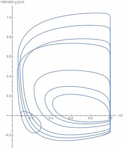Here, we numerically solving (21) which is a nonlinear transformed version of (8), with MATHEMATICA. 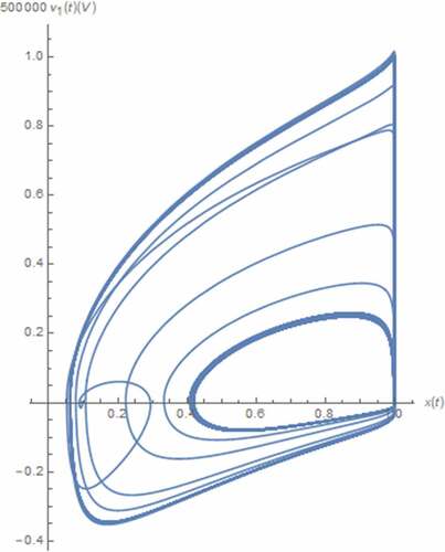Based on the obtained solutions, the dynamics and phase portraits of i₁(t), i₂(t), x(t), and v₁(t) can be simulated by keeping the above relationship between t and $\xi$ along with those between the normal and nonlinear transformed electrical quantities in mind as depicted in Fig. 2–11 where the axis scaling has been applied to Figs. 8, 9, and 11 for visibility. From Figure 4, the boundary effect of the memristive device on x(t) can be seen. Moreover, the strange attractors which indicate the chaotic behavior can be observed from Fig. 5–11. Noted that a pinched hysteresis behavior can be from the strange attractor depicted Figure 6 where i₁(t) is the current flowing through the memristive device which is passive as the attractor is located in quadrants 1 and 3, and v₁(t) is partly composed of the voltage across such device. It can also be seen that those x(t) related attractors depicted in Figs. 8, 9 and 11 are restricted due to the boundary effect. Unlike those of the integer circuit, these restrictions occur at x(t) = 1 only. This is because the minimum value of x(t) is greater than 0 as can be seen from Figure 3.

Figure 2. I₁(t) v.s. t

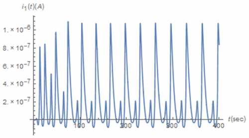
Figure 3. I₂(t) v.s. t

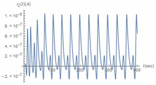
Figure 4. X(t) v.s. t

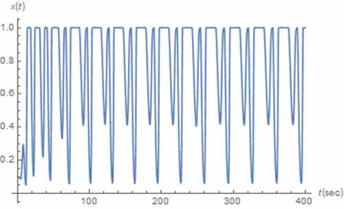
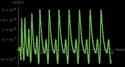
Figure 5. V₁(t) v.s t

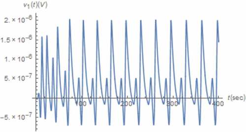
Figure 6. I₁(t) v.s. v₁(t)

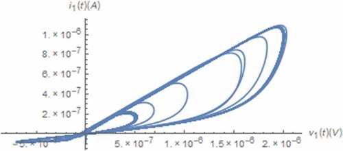
Figure 7. I₂(t) v.s. v₁(t)

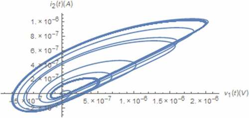
Figure 8. I₁(t) v.s. x(t)

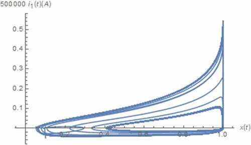
Figure 9. I₂(t) v.s. x(t)

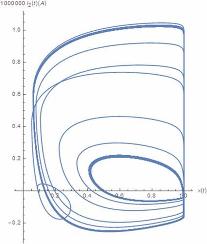
Figure 10. I₂(t) v.s. i₁(t)

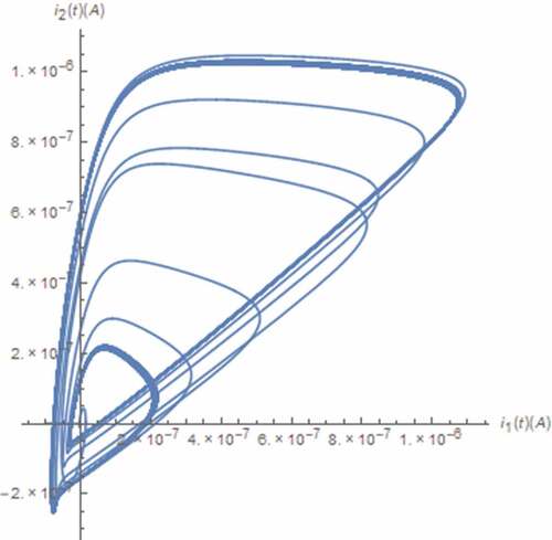
Figure 11. V₁(t) v.s. x(t)

For the quantitative analysis, the Lyapunov exponents and dimension must be evaluated. First, the system’s variational equation must be formulated by employing the following theorem (Hartl, 2003).

Theorem 2: For arbitrary dynamical system given by

(22) $\frac{\mathrm{d}}{\mathrm{d}\xi }\mathbf{X}(\xi )=\mathbf{F}(\mathbf{X}(\xi ))$(22)

where $\mathbf{X}(\xi )=[\begin{array}{cccc}{X}_1(t)& X_2(\xi )& \cdots & X_N(\xi )\end{array}{]}^T$ and $\mathbf{F}(\mathbf{X}(\xi ))=\left[\begin{array}{c}{F}_1(X_1(\xi ),X_2(\xi ),..,X_N(\xi ))\\ F_2(X_1(\xi ),X_2(\xi ),..,X_N(\xi ))\\ ⋮\\ F_N(X_1(\xi ),X_2(\xi ),..,X_N(\xi ))\end{array}\right]$, its variational equation can be given by (23) where $\mathbf{D}(\xi )={\left[\begin{array}{cccc}{\mathbf{d}}_1(\xi )& {\mathbf{d}}_2(\xi )& \cdots & {\mathbf{d}}_N(\xi )\end{array}\right]}^T$, $\mathbf{U}(\xi )=\left[\begin{array}{cccc}{\mathbf{u}}_1(\xi )& {\mathbf{u}}_2(\xi )& \cdots & {\mathbf{u}}_N(\xi )\end{array}\right]$ and ${\mathbf{d}}_j(\xi )=\left[\begin{array}{c}\frac{\mathrm{\partial }}{\mathrm{\partial }{X}_1(\xi )}{F}_j(X_1(\xi ),X_2(\xi ),..,X_N(\xi )\\ \frac{\mathrm{\partial }}{\mathrm{\partial }{X}_2(\xi )}{F}_j(X_1(\xi ),X_2(\xi ),..,X_N(\xi )\\ \hspace{0.17em}\\ \frac{\mathrm{\partial }}{\mathrm{\partial }{X}_N(\xi )}{F}_j(X_1(\xi ),X_2(\xi ),..,X_N(\xi )\end{array}\right]$. Noted that${\mathbf{u}}_j(\xi )$where {j} = {1, 2, …, N} stands for the j^th tangent vector of the system’s trajectory in an N dimensional space defined by (X₁(ξ), X₂(ξ), …, X_N(ξ)). Moreover,${\mathbf{u}}_j(\xi )$’s are both linearly independent and orthonormal.

(23) $\frac{\mathrm{d}}{\mathrm{d}\xi }\mathbf{U}(\xi )=\mathbf{D}(\xi )\mathbf{U}(\xi )$(23)

After simultaneously solving (22) and (23), the Lyapunov exponents and dimensions can be determined from the following definitions.

Definitions 3: For arbitrary dynamical system, its j^th Lyapunov exponent (LE_j) can be given by (Wolf et al., 1985)

(24) $L{E}_j=\underset{\xi \to \mathrm{\infty }}{lim}\frac{1}{\xi }ln[\frac{{\mathbf{u}}_j(\xi )}{{\mathbf{u}}_j(0)}]$(24)

where denotes the Euclidian norm operator.

Definitions 4: Given the Lyapunov exponents, the Lyapunov dimension (D_L) can be found as (Mahmoud et al., 2009)

(25) $D_L=K-\frac{\sum _{j=1}^K[L{E}_j]}{L{E}_{j+1}}$(25)

where K is the largest integer such that $\sum _{j=1}^K[L{E}_j]>0$.

At this point, the quantitative analysis of generalized circuit can be performed as follows.

Example 2: Let all parameters and initial values be similar to those assumed in example 1. For the generalized circuit, there exists four Lyapunov exponents i.e. LE₁, LE₂, LE_3, and LE₄. After applying theorem 2 and corollary 2.1 to (21), LE₁, LE₂, LE_3, and LE₄ can be obtained via numerical calculation with MATHEMATICA as given in Table 1. Since LE₁ > 0 and LE₁ + LE₂ + LE₃ + LE₄ < 0, both expansion in one direction and contracting volumes in the phase space of the attractor which indicates the chaotic behavior can be observed. We have also found that the contraction outweighs the expansion because LE₁ + LE₂ + LE₃ + LE₄ < 0; therefore, the generalized circuit is dissipative. Moreover, D_L can be obtained after applying corollary 2.2 to LE₁, LE₂, LE_3, and LE₄ as fractional number which indicates that manifold in the phase space is a strange attractor, as can be seen from Table 1.

Table 1. LE₁, LE₂, LE₃, LE₄ and D_L of the generalized circuit with dimensional consistency awareness

LE1	0.070961
LE2	−0.057483
LE3	−2.492179
LE4	−16.982975
LE1 + LE2 + LE3 + LE4	−19.461676
DL	2.005408

For obtaining the necessary criteria for the generalized circuit to remain chaotic, the linear equivalence of (8) must be determined. Since it can be seen from (8) that

$g_1(i_1(t),i_2(t),x(t),v_1(t))=\frac{1}{L_{1\alpha }}[v_1(t)-(M_{on}x(t)-M_{off}(1-x(t)))i_1(t)]$

(26) $g_2(i_1(t),i_2(t),x(t),v_1(t))=\frac{R}{L_{2\alpha }}{i}_2(t)-\frac{1}{L_{2\alpha }}{v}_1(t)$(26)

$\begin{array}{c}{g}_3(i_1(t),i_2(t),x(t),v_1(t))\\ =k_{\alpha }(1-{[}^{a^2{(}^{ax(t)-\mathrm{u}(-i_1(t)))2}+(1-a^2)]p})i_1(t)\end{array}$

$g_4(i_1(t),i_2(t),x(t),v_1(t))=\frac{1}{C_{1\alpha }}(i_2(t)-i_1(t))$

we have E = (0, 0, 0, χ) similarly to the integer circuit; thus, the linear equivalence of (8) can be given by (10) with N = 4 and$\mathbf{x}(t)=(i_1(t),i_2(t),x(t),v_1(t))$. However, ${\mathbf{J}}_{\mathbf{E}}=\left[\begin{array}{cccc}-(M_{on}\chi -M_{off}(1-\chi )/L_{1\alpha }& 0& 0& 1/L_{1\alpha }\\ 0& R/L_{2\alpha }& 0& -1/L_{2\alpha }\\ k_{\alpha }(1-{[a^2{(\chi -1)}^2+(1-a^2)]}^p)& 0& 0& 0\\ -1/C_{1\alpha }& 1/C_{1\alpha }& 0& 0\end{array}\right]$ must be adopted. As a result, the characteristic equation of (8) can also be given by (14) but with A = (L_2αM_off − L_1αR − L_2αM_offχ + L_2α M_onχ)/L_1αL_2α, B = (L_1α − L_2α + C_1αM_offR −C_1αM_offR χ + C_1α M_onR χ)/C_1αL_1αL_2α and C = (M_off − R − M_off χ + M_on χ)/C_1αL_1α L_2α instead. Therefore ${\lambda }_1$, ${\lambda }_2$, ${\lambda }_3$ and ${\lambda }_4$ of the generalized circuit have been found to be similar to those of the integer-order circuit presented above but with c + a = (L_2α M_off − L_1αR − L_2αM_offχ + L_2α M_onχ)/L_1α L_2α, ac+b = (L_1α − L_2α + C_1αM_offR −C_1α M_offR χ + C_1α M_onR χ)/C_1αL_1αL_2α and bc = (M_off − R − M_off χ + M_on χ)/C_1αL_1α L_2α. For the circuit to be chaotic, E must be an unstable saddle focus thus

$c>0$

(27) $a<0$(27)

$\alpha \ge \frac{2}{\pi }{tan}^{-1}[\frac{2}{a}\sqrt{b-\frac{a^2}{4}}]$

must be simultaneously satisfied; otherwise, it will ceases to be chaotic as illustrated in the following example.

Example 3: In this example, we will show that the generalized circuit ceases to be chaotic if the criterion on α as given by (27) is violated. Since we adopt all parameters assumed in Example 1, it can be seen from (27) that α ≥ 0.728 must be satisfied for satisfying the criterion on α; thus, the circuit remains chaotic. As a result, we will demonstrate that E ceases to be an unstable saddle focus because the stable region has been enlarged so that it covers all eigenvalues; thus, the circuit ceases to be chaotic if α < 0.728. In order to do so, we formulate

(28) $m_i=\frac{\alpha \pi }{2}-\left|arg[{\lambda }_i]\right|$(28)

where {i} = {2, 3, 4} as the representative of λ₂, λ₃ and λ₄ because the effect of $m_i$ to the location of λ_i on the complex plane is equivalent to that of Re[λ_i] if λ_i is an eigenvalue for the integer-order circuit (Banchuin, 2020), (Abdelouahab et al., 2012). Noted also that we do not need to formulate m₁ as λ₁ = 0; thus, its location cannot be altered by any parameter changing. By applying λ₂, λ₃ and λ₄ to (28), we have

(29) $m_2=\left(\frac{\alpha }{2}-1\right)\pi$(29)

(30) $m_{3,4}=\frac{\alpha \pi }{2}-{tan}^{-1}[\frac{2}{a}\sqrt{b-\frac{a^2}{4}}]$(30)

Noted that $m_3=m_4$thus they are commonly referred to as $m_{3,4}$for simplicity. Since the plots of’s against bifurcation parameters have been used for studying the dynamic of fractional-order circuit (Banchuin, 2020) due to the aforesaid equivalence of$m_i$’s and Re[λ_i]’s (if λ_i’s are eigenvalues of the integer-order system) and the previous usages of the similar plots of Re[λ_i]’s for studying the integer-order systems (De Ninno & Fanelli, 2004), (Yuan & Wang, 2016), we adopt the mentioned fractional-order circuit dedicated approach in this work. As the criterion on α has been considered, we choose α as our bifurcation parameters and thus the dynamics of $m_2$, $m_3$ and $m_4$can be simulated as depicted in Figs. 12 and 13 which shows that $m_2<0$ always unlike $m_3$ and $m_4$. Therefore, the circuit’s stability is solely governed by λ₃ and λ₄ as λ₁ always be at the origin at the origin and λ₂ always be in the stable region of the complex plane.

Figure 12. $m_2$ v.s. α.

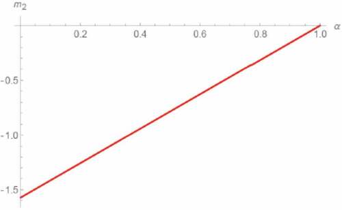
Figure 13. $m_{3,4}$v.s. α.

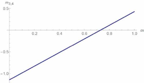
From Figure 13, it can be seen that E ceases to be an unstable saddle focus; thus, the generalized circuit ceases to be chaotic when $\alpha <$0.728 and vice versa as $m_{3,4}<0$and $m_{3,4}>0$which, respectively, imply that both λ₃ and λ₄ are in stable and unstable region and can be observed. In addition, we have also found that the transversality criterion is established at 0.728 because $m_{3,4}=0$ where$\frac{\mathrm{\partial }}{\mathrm{\partial }\alpha }{m}_{3,4}{|}_{\alpha =0.728}=\frac{\pi }{2}\ne 0$. As a result, it can be stated based on the fractional-order Hopf bifurcation criteria (Abdelouahab et al., 2012) that both λ₃ and λ₄ cross the boundary between stable and unstable region with non-zero speed; thus, the circuit’s stability switches, its dynamical behavior changes and the circuit undergoes a Hopf bifurcation through E and at α = 0.728. If we let $\alpha =$0.5, the phase portraits of $i_2(t)$and $x(t)$ can be simulated as depicted in Figure 14 where an axis scaling has been applied again for visibility and a limit cycle can be observed instead of a chaotic attractor. Before we proceed further, it should be mentioned here that the generalized circuit can never be locally asymptotically stable but merely marginally stable. This is because λ₁ always be at the origin of the complex plane which locates on the stability boundary.

Figure 14. I₂(t) v.s. x(t): α = 0.5

Finally, we will assert the importance of dimensional consistency awareness. In order to do so, we derive the dynamical equation of the generalized circuit without such awareness by applying (31) to (5). As a result, (32) has been obtained then we numerically determine the associated LE₁, LE₂, LE₃, LE₄ and D_L by applying the nonlinear transformation, theorem 2 and corollaries 2.1 and 2.2 to (32). The resulting LE₁, LE₂, LE₃, LE₄ and D_L are different from those of the circuit with dimensional consistency awareness as can be seen from Table 2. These differences imply the different amounts of expansion and contraction along with the fractal dimension-phase space manifolds thus assert the importance of dimensional consistency awareness to the dynamical behavior of the obtained fractional-order circuit previously proposed (Banchuin, 2020).

(31) $\frac{\mathrm{d}}{\mathrm{d}t}\to {\mathrm{D}}_t^{\alpha }$(31)

${\mathrm{D}}_t^{\alpha }{i}_1(t)=\frac{1}{L_1}[v_1(t)-(M_{on}x(t)-M_{off}(1-x(t)))i_1(t)]$

(32) ${\mathrm{D}}_t^{\alpha }{i}_2(t)=\frac{R}{L_2}{i}_2(t)-\frac{1}{L_2}{v}_1(t)$(32)

${\mathrm{D}}_t^{\alpha }x(t)=k(1-[a^2(x(t)-\mathrm{u}(-i_1(t)){)}^2+(1-a^2){]}^p)i_1(t)$

Table 2. LE₁, LE₂, LE₃, LE₄ and D_L of the generalized circuit without dimensional consistency awareness

LE1	0.027962
LE2	−0.070488
LE3	−2.549971
LE4	`-17.29119
LE1 + LE2 + LE3 + LE4	−19.883687
DL	1.396689

5. The circuit realization and emulator implemantation

By inspecting (8), it has been found that the generalized circuit can be realized as a circuit with a similar structure to the integer-order circuit but with all circuit elements except the negative resistor be replaced by their fractional-order counterparts i.e. fractional-order inductor, fractional-order capacitor and fractional-order HP memristor. This is because$k_{\alpha }$characterizes the fractional-order HP memristor (Banchuin, 2018). Moreover, $C_{1\alpha }$ is physically the pseudo-capacitance which characterizes the fractional-order capacitor (Freeborn et al., 2013), where $L_{1\alpha }$and $L_{2\alpha }$ are physically the inductivity which characterize the fractional-order inductor (Schäfer & Krüger, 2006). For simplicity, a fractional-order memristor emulator (Rashad et al., 2017) with proper circuit parameter adjustment could serve as the fractional-order HP memristor as it is also current controlled with quadrants 1 and 3 resided single pinched point hysteresis loop. Compared with the previous fractional-order HP memristor-based chaotic circuit, our generalized circuit is simpler as merely a single fractional-order HP memristor is required apart from being dimensional consistent. Therefore, it is the simplest fractional-order HP memristor-based chaotic circuit. By this virtue and its dimensional consistency awareness, our generalized circuit has been found to be an interesting example of fractional-order chaotic circuits. Thus, it is beneficial to those fractional-order chaotic circuit and system-related research areas.

In order to implement the circuit emulator, it is convenient to, respectively, substituting i₁(t), i₂(t) and v₁(t) in (8) by y(t), z(t) and w(t) which in turn do not assume specific physical meanings. Therefore, (8) can be rewritten as

${\mathrm{D}}_t^{\alpha }x(t)=k_{\alpha }\mathrm{f}(x(t),y(t))y(t)$

${\mathrm{D}}_t^{\beta }y(t)=\frac{1}{L_{1\beta }}[w(t)-(M_{on}x(t)-M_{off}(1-x(t)))y(t)]$

(33) ${\mathrm{D}}_t^{\gamma }z(t)=\frac{R}{L_{2\gamma }}z(t)-\frac{1}{L_{2\gamma }}w(t)$(33)

${\mathrm{D}}_t^{\delta }w(t)=\frac{1}{C_{1\delta }}(z(t)-y(t))$

where 0 < β ≤ 1, 0 < γ ≤ 1, 0 < δ ≤ 1 and f(x(t),y(t)) can be given by (4) with i(t) = y(t). Noted that the order of the fractional derivative has been allowed to be incommensurate for obtaining full degree of freedom in the implementation. As a result, L_1α, L_2α and C_1α become L_1β, L_2γ and C_1δ which can be, respectively, given by, $L_{2\gamma }=L_2{\sigma }^{\gamma -1}$and $C_{1\delta }=C_1{\sigma }^{\delta -1}$ for maintaining the dimensional consistency. Obviously, (33) can be recast to

$x(t)=k_{\alpha }{\mathrm{J}}_t^{\alpha }[\mathrm{f}(x(t),y(t))y(t)]$

$y(t)=\frac{1}{L_{1\beta }}{\mathrm{J}}_t^{\beta }[w(t)-(M_{on}x(t)-M_{off}(1-x(t)))y(t)]$

(34) $z(t)=\frac{1}{L_{2\gamma }}{\mathrm{J}}_t^{\gamma }[Rz(t)-w(t)]$(34)

$w(t)=\frac{1}{C_{1\delta }}{\mathrm{J}}_t^{\delta }[z(t)-y(t)]$

where ${\mathrm{J}}_t^{\alpha }\stackrel{\mathrm{\Delta }}{=}{\mathrm{D}}_t^{-\alpha }$, ${\mathrm{J}}_t^{\beta }\stackrel{\mathrm{\Delta }}{=}{\mathrm{D}}_t^{-\beta }$, ${\mathrm{J}}_t^{\gamma }\stackrel{\mathrm{\Delta }}{=}{\mathrm{D}}_t^{-\gamma }$ and ${\mathrm{J}}_t^{\delta }\stackrel{\mathrm{\Delta }}{=}{\mathrm{D}}_t^{-\delta }$. By inspecting (34), the emulator’s block diagram can be obtained as depicted in Figure 15. Based on this block diagram, the emulator circuit can be implemented by merely applying of the shelf components. An example of emulator circuits is depicted in Figure 16 where x(t), y(t), z(t) and w(t) are physically voltages. Therefore, TL084 and AD633 which operates in the voltage mode can be applied as our OPAMP and multiplier and. In addition, C_α, C_β, C_γ and C_δ stand for the fractional-order capacitors of order α, β, γ and δ with the following pseudo-capacitances

$C_{\alpha }=0.001/k_{\alpha }$

(35) $C_{\beta }=0.001L_{1\beta }$(35)

$C_{\gamma }=0.001L_{2\gamma }$

$C_{\delta }=0.001C_{1\delta }$

Figure 15. The emulator block diagram

Figure 16. The emulator circuit

Moreover, the resistance values can be given by

$r_1=1000/M_{off}$

(36) $r_2=1000/(M_{on}+M_{off})$(36)

$r_3=1000/R$

For implementing the fractional-order capacitors, the RC approximated circuit of a constant phase element (CPE) (Petrzela, 2019) depicted here in Figure 17 has been found to be applicable as a fractional-order capacitor is a CPE. According to Petrzela, (2019), the parameters of such circuit must satisfy

(37) $s^{\chi }{C}_{\chi }=s{C}_p+R_p^{-1}+\sum _{k=1}^7\frac{s{C}_k}{s{C}_k{R}_k+1}$(37)

Figure 17. The RC approximated circuit of a CPE (Petrzela, 2019)

where {χ} = {α, β, γ, δ}.

In the following example, the simulation results will be illustrated.

Example 4: Let us assume a set of parameters similar to that of Example 1 and given β = 0.8, γ = 0.95 and δ = 0.85. The resulting parameters of the emulator circuit can be summarized in Table 3 where the resistance and pseudo-capacitance values have been evaluated via (35) and (36). The corresponding values of resistances and capacitances for the RC approximated circuits as summarized in Table 4-7-VII have been determined via (37) by fitting its coefficient to the data based on the pseudo-capacitances and orders presented in Table 3 with the least squares method. The simulated dynamics of$x(t)$,$y(t)$,$z(t)$ and w(t) can be obtained as depicted in Fig. 18–21. Similarly to Example 1, the chaotic waveforms with boundary restriction at x(t) = 1 can be observed. However, these waveforms employ different frequencies as α, β, γ and δ are incommensurate where $z(t)$oscillates at the highest frequency followed by $x(t)$, w(t) and$y(t)$.

Table 3. The parameter values of emulator circuit

Parameter	Value
r1	100 Ω
r2	85 Ω
r3	577 Ω
Cα	50.832 pFsec^α−1
Cβ	254.16 μFsec^β^−1
Cγ	1355.2 μFsec^γ−1
Cδ	410.02 μFsec^δ−1
α	0.9
β	0.8
γ	0.95
δ	0.85

Table 4. The resistance and capacitance values for approximating C_α

R1	1.63066 MΩ
R2	1.63605 MΩ
R3	1.64563 MΩ
R4	1.64042 MΩ
R5	1.63610 MΩ
R6	1.63589 MΩ
R7	1.63553 MΩ
Rp	1.81203 MΩ
C1	0.579643 μF
C2	0.579664 μF
C3	0.579307 μF
C4	0.579500 μF
C5	0.579662 μF
C6	0.579670 μF
C7	0.579684 μF
Cp	0.167286 μF

Table 5. The resistance and capacitance values for approximating C_β

R1	2.48600 Ω
R2	2.58296 Ω
R3	2.15415 Ω
R4	2.50960 Ω
R5	2.55557 Ω
R6	2.53964 Ω
R7	2.74010 Ω
Rp	191.187 Ω
C1	1 μF
C2	1 μF
C3	1 μF
C4	1 μF
C5	1 μF
C6	1 μF
C7	1 μF
Cp	1 μF

Table 6. The resistance and capacitance values for approximating C_γ

R1	1.24863 Ω
R2	1.24863 Ω
R3	1.24863 Ω
R4	1.24863 Ω
R5	1.24863 Ω
R6	1.24863 Ω
R7	1.24863 Ω
Rp	95.2000 Ω
C1	1 μF
C2	1 μF
C3	1 μF
C4	1 μF
C5	1 μF
C6	1 μF
C7	1 μF
Cp	1 μF

Table 7. The resistance and capacitance values for approximating C_δ

R1	133.071 Ω
R2	16.2204 Ω
R3	18.1372 Ω
R4	15.8298 Ω
R5	20.9668 Ω
R6	40.8958 Ω
R7	34.8016 Ω
Rp	93.4220 Ω
C1	1 μF
C2	1 μF
C3	1 μF
C4	1 μF
C5	1 μF
C6	1 μF
C7	1 μF
Cp	1 μF

Figure 18. X(t) v.s. t

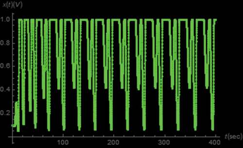
Figure 19. Y(t) v.s. t

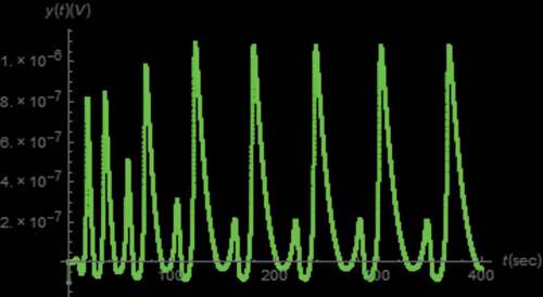
Figure 20. Z(t) v.s. t

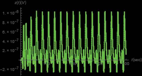
Figure 21. W(t) v.s. t

6. Conclusion

In this work, a dimensional consistency aware fractional-order generalization of HP memristor-based chaotic circuit has been performed with the physical meaning of fractional time component assigned. The simplest autonomous circuit based on such memristor with correct memristor assumption has been chosen as the candidate circuit where a novel fractional-order HP memristor dedicated window function has been adopted for modelling the boundary effect. The dynamic of the generalized circuit has been analyzed where the importance of dimensional consistency awareness has been asserted. The realization of the circuit by using the fractional-order elements is indicated. Apart from being dimensional consistent, the indicated circuit has been found to be the simplest fractional-order HP memristor-based chaotic circuit. The fractional-order capacitor-based circuit emulator has been presented where we have shown that the oscillating frequencies of the responses are depended on the orders of fractional-order capacitors. At this point, it can be seen that this work is beneficial to those research areas including the analysis and design of chaotic circuits, fractional-order circuits, HP memristor-based circuits and nonlinear circuits and so on. In addition, a similar study based on other often cited fractional derivatives e.g., the above-mentioned fractional derivatives with nonsingular and nonlocal-nonsingular kernels and conformable fractional derivative etc., has been found to be an interesting further study. A generalization of the commercially available KNOWNM memristor-based chaotic circuit (C. Volos et al., 2020, September), (C. K. Volos et al., 2020) is also a challenging open research question.

Data availability statement

The data supporting the finding of this study are available within the article.

Additional information

Funding

The author received no direct funding for this research.

Notes on contributors

Rawid Banchuin

Assoc. Prof. Dr. Rawid Banchuin is currently with the Graduated School of Information Technology and Faculty of Engineering, Siam University, Bangkok, Thailand. His major research of interest is the mathematical analysis of electrical/electronic elements and circuits including the fractional order elements, the elements with memory, the fractional order circuits, the fractal circuits, the chaotic circuits and other nonlinear circuits.

References

- Abdelouahab, M. S., Hamri, N. E., & Wang, J. (2012). Hopf bifurcation and chaos in fractional-order modified hybrid optical system. Nonlinear Dynamics, 69 (1–2), 275–28. https://doi.org/10.1007/s11071-011-0263-4
- Abdelouahab, M. S., & Lozi, R. (2015, May). Bifurcation analysis and chaos in simplest fractional-order electrical circuit. In 2015 3rd International Conference on Control, Engineering & Information Technology (CEIT) (pp. 1–5). IEEE. https://doi.org/10.1109/CEIT.2015.7233122
- Ahmadi, S., & Azhari, S. J. (2018). A novel fully differential second generation current conveyor and its application as a very high CMRR instrumentation amplifier. Emerging Science Journal, 2(2), 85–92. https://doi.org/10.28991/esj-2018-01131
- Alkahtani, B. S. T. (2016). Chua’s circuit model with Atangana–Baleanu derivative with fractional order. Chaos, Solitons, and Fractals, 89, 547–551. https://doi.org/10.1016/j.chaos.2016.03.020
- Atangana, A., & Alkahtani, B. S. T. (2015). Extension of the resistance, inductance, capacitance electrical circuit to fractional derivative without singular kernel. Advances in Mechanical Engineering, 7 (6), 1687814015591937. https://doi.org/10.1177/1687814015591937
- Atangana, A., & Baleanu, D. (2016). New fractional derivatives with nonlocal and non-singular kernel: Theory and application to heat transfer model, Thermal Science, 20(2), 763–769. https://doi.org/10.2298/TSCI160111018A
- Atangana, A., & Secer, A. (2013, March). A note on fractional order derivatives and table of fractional derivatives of some special functions. In Abstract and applied analysis (2013). Hindawi. https://doi.org/10.1155/2013/279681
- Banchuin, R. (2018). On the memristances, parameters, and analysis of the fractional order memristor. Active and Passive Electronic Components, 2018. Retrieved from. 2018: 1–14. https://doi.org/10.1155/2018/3408480.
- Banchuin, R. (2020). On the dimensional consistency aware fractional domain generalization of simplest chaotic circuits. Mathematical Problems in Engineering, 2020. Retrieved from. 2020: 1–20. https://doi.org/10.1155/2020/9862158.
- Biolek, Z., Biolek, D., & Biolkova, V. (2009). SPICE model of memristor with nonlinear dopant drift. Radioengineering, 182, 210–214. https://www.radioeng.cz/fulltexts/2009/09_02_210_214.pdf
- Buscarino, A., Fortuna, L., Frasca, M., & Valentina Gambuzza, L. (2012). A chaotic circuit based on Hewlett-Packard memristor. Chaos: An Interdisciplinary Journal of Nonlinear Science, 22 (2), 023136. https://doi.org/10.1063/1.4729135
- Cafagna, D., & Grassi, G. (2012). On the simplest fractional-order memristor-based chaotic system. Nonlinear Dynamics, 70 (2), 1185–1197. https://doi.org/10.1007/s11071-012-0522-z
- Caputo, M., & Fabrizio, M. (2015). A new definition of fractional derivative without singular kernel. Progress in Fractional Differentiation and Applications, 1(2), 1–13. https://doi.org/10.2298/TSCI151224222Y
- Chu, T., Chua, A., & Secco, E. L. (2020). A Wearable MYO Gesture Armband Controlling Sphero BB-8 Robot. HighTech and Innovation Journal, 1(4), 179–186. https://doi.org/10.28991/HIJ-2020-01-04-05
- Chua, L. (1971). Memristor-the missing circuit element. IEEE Transactions on Circuit Theory, 18(5), 507–519. https://doi.org/10.1109/TCT.1971.1083337
- De Ninno, G., & Fanelli, D. (2004). Controlled Hopf Bifurcation of a storage-ring free-electron laser. Physical Review Letters, 92 (9), 094801. https://doi.org/10.1103/PhysRevLett.92.094801
- Deng, H., & Wang, Q. (2013). Dynamics and synchronization of memristor-based fractional-order system. International Journal of Modern Nonlinear Theory and Application, 2(4), 223. https://doi.org/10.4236/ijmnta.2013.24031
- Freeborn, T. J., Maundy, B., & Elwakil, A. S. (2013). Measurement of supercapacitor fractional-order model parameters from voltage-excited step response. IEEE Journal on Emerging and Selected Topics in Circuits and Systems, 3(3), 367–376. https://doi.org/10.1109/JETCAS.2013.2271433
- Gómez, F., Rosales, J., & Guía, M. (2013). RLC electrical circuit of non-integer order. Open Physics, 11 (10), 1361–1365. https://doi.org/10.2478/s11534-013-0265-6
- Gómez‐Aguilar, J. F., Atangana, A., & Morales‐Delgado, V. F. (2017). Electrical circuits RC, LC, and RL described by Atangana–Baleanu fractional derivatives. International Journal of Circuit Theory and Applications, 45(11), 1514–1533. https://doi.org/10.1002/cta.2348 Retrieved from
- Gómez-Aguilar, J. F., Rosales-García, J., Razo-Hernández, J. R., & Guía-Calderón, M. (2014). Fractional RC and LC electrical circuits. Ingeniería. Investigación Y Tecnología, 152, 311–319. https://doi.org/10.1016/S1405-77431472219-X
- Guang-Yi, W., Jie-Ling, H., Fang, Y., & Cun-Jian, P. (2013). Dynamical behaviors of a TiO2 memristor oscillator. Chinese Physics Letters, 30(11), 110506. https://doi.org/10.1088/0256-307X/30/11/110506
- Hartl, M. D. (2003). Lyapunov exponents in constrained and unconstrained ordinary differential equations (No. physics/0303077). https://cds.cern.ch/record/609829
- Jin, P., Wang, G., Iu, H. H. C., & Fernando, T. (2017). A locally active memristor and its application in a chaotic circuit. IEEE Transactions on Circuits and Systems II: Express Briefs, 65(2), 246–250. https://doi.org/10.1109/TCSII.2017.2735448
- Joglekar, Y. N., & Wolf, S. J. (2009). The elusive memristor: Properties of basic electrical circuits, European Journal of Physics, 30(4), 661. https://doi.org/10.1088/0143-0807/30/4/001
- Jumarie, G. (2006). Modified Riemann-Liouville derivative and fractional Taylor series of nondifferentiable functions further results. Computers & Mathematics with Applications, 51 (9–10), 1367–1376. https://doi.org/10.1155/2013/279681
- Khalil, R., Al Horani, M., Yousef, A., & Sababheh, M. (2014). A new definition of fractional derivative. Journal of Computational and Applied Mathematics, 264, 65–70. https://doi.org/10.1016/j.cam.2014.01.002.
- Mahmoud, G. M., Farghaly, A. A., & Shoreh, A. H. A technique for studying a class of fractional-order nonlinear dynamical systems. (2017). International Journal of Bifurcation and Chaos, 27(9), 1750144. https://doi.org/10.1142/S0218127417501449
- Mahmoud, G. M., Mahmoud, E. E., & Ahmed, M. E. (2009). On the hyperchaotic complex Lü system. Nonlinear Dynamics, 58 (4), 725–738. https://doi.org/10.1007/s11071-009-9513-0
- Martinez, L., Rosales, J. J., Carreño, C. A., & Lozano, J. M. (2018). Electrical circuits described by fractional conformable derivative. International Journal of Circuit Theory and Applications, 46 (5), 1091–1100. https://doi.org/10.1002/cta.2475
- Muthuswamy, B., & Chua, L. O. (2010). Simplest chaotic circuit. International Journal of Bifurcation and Chaos, 20 (5), 1567–1580. https://doi.org/10.1142/S0218127410027076
- Omidi, A., Karami, R., Emadi, P. S., & Moradi, H. (2017). Design of the low noise amplifier circuit in band L for improve the gain and circuit stability. Emerging Science Journal, 1(4), 192–200. https://doi.org/10.28991/ijse-01122
- Petrzela, J. (2019). Accurate constant phase elements dedicated for audio signal processing. Applied Sciences, 9 (22), 4888. https://doi.org/10.3390/app9224888
- Prodromakis, T., Peh, B. P., Papavassiliou, C., & Toumazou, C. (2011). A versatile memristor model with nonlinear dopant kinetics. IEEE Transactions on Electron Devices, 58(9), 3099–3105. https://doi.org/10.1109/TED.2011.2158004
- Rashad, S. H., Hamed, E. M., Fouda, M. E., AbdelAty, A. M., Said, L. A., & Radwan, A. G. (2017, May). On the analysis of current-controlled fractional-order memristor emulator. In 2017 6th International Conference on Modern Circuits and Systems Technologies (MOCAST) (pp. 1–4). IEEE. https://doi.org/10.1109/MOCAST.2017.7937670
- Schäfer, I., & Krüger, K. (2006). Modelling of coils using fractional derivatives. Journal of Magnetism and Magnetic Materials, 307 (1), 91–98. https://doi.org/10.1016/j.jmmm.2006.03.046
- Shang, Y. (2012). A lie algebra approach to susceptible-infected-susceptible epidemics. Electronic Journal of Differential Equations, 2012233, 1–7. http://ejde.math.txstate.edu
- Shang, Y. (2014). Vulnerability of networks: Fractional percolation on random graphs. Physical Review E, 89(1), 0128131–0128134. https://doi.org/10.1103/PhysRevE.89.012813
- Shi, M., Yu, Y., & Xu, Q. (2018). Window function for fractional-order HP TiO2 non-linear memristor model. IET Circuits, Devices & Systems, 12(4), 447–452. https://doi.org/10.1049/iet-cds.2017.0414
- Shotorbani, A. R., & Saghai, H. R. (2018). Modeling and implementing nonlinear equations in solid-state lasers for studying their performance. Emerging Science Journal, 2(2), 78–84. http://dx.doi.org/10.28991/esj-2018-01130
- Strukov, D. B., Snider, G. S., Stewart, D. R., & Williams, R. S. (2008). The missing memristor found. Nature, 453 (7191), 80. https://doi.org/10.1038/nature06932
- Teng, L., Iu, H. H., Wang, X., & Wang, X. (2014). Chaotic behavior in fractional-order memristor-based simplest chaotic circuit using fourth degree polynomial. Nonlinear Dynamics, 77 (1–2), 231–241. https://doi.org/10.1007/s11071-014-1286-4
- Volos, C., Nistazakis, H., Pham, V. T., & Stouboulos, I. (2020, September). The first experimental evidence of chaos from a nonlinear circuit with a real memristor. In 2020 9th International Conference on Modern Circuits and Systems Technologies (MOCAST) (pp. 1–4). IEEE. https://doi.org/10.1109/MOCAST49295.2020.9200269
- Volos, C. K., Pham, V. T., Nistazakis, H. E., & Stouboulos, I. N. (2020). A dream that has come true: chaos from a nonlinear circuit with a real memristor. International Journal of Bifurcation and Chaos, 30(13), 2030036. https://doi.org/10.1142/S0218127420300360
- Wang, G., Cui, M., Cai, B., Wang, X., & Hu, T. (2015). A chaotic oscillator based on HP memristor model. Mathematical Problems in Engineering, 2015. https://doi.org/10.1155/2015/561901.
- Wang, Z., Sun, C., Jin, F., Mo, W., Song, J., & Dong, K. (2018a, May). Chaotic oscillator based on a modified voltage-controlled hp memristor model. In 2018 2nd IEEE Advanced Information Management, Communicates, Electronic and Automation Control Conference (IMCEC) (pp. 153–156). IEEE. https://doi.org/10.1109/IMCEC.2018.8469486
- Wang, Z., Sun, C., Jin, F., Mo, W., Song, J., & Dong, K. (2018b). A widely amplitude-adjustable chaotic oscillator based on a physical model of HP memristor. IEICE Electronics Express, 15(8), 20171251. https://doi.org/10.1587/elex.15.20171251
- Wolf, A., Swift, J. B., Swinney, H. L., & Vastano, J. A. (1985). Determining Lyapunov exponents from a time series. Physica D. Nonlinear Phenomena, 16 (3), 285–317. https://doi.org/10.1016/0167-27898590011-9
- Yang, C., Cai, H., & Zhou, P. (2016). Stabilization of the fractional-order chua chaotic circuit via the Caputo derivative of a single input. Discrete Dynamics in Nature and Society, 2016. Retrieved from. 2016: 1–5. https://doi.org/10.1155/2016/4129756.
- Yuan, C., & Wang, J. (2016). Hopf bifurcation analysis and control of three-dimensional Prescott neuron model. Journal of Vibroengineering, 18 (6), 4105–4115. https://doi.org/10.21595/jve.2016.16933