Numerical simulation of inverse geochemistry problems by regularizing algorithms

Abstract

Currently, methods and approaches of scientific visualization based on additional data analysis are being intensively developed due to the rapid development of computer technology in geology. The general concept is that the main data field on the day surface and additional conditions are specified at the input. Further, the methods of mathematical geophysics are used for their analysis and processing, as a result of which new information is obtained for deep exploration. Then visualization tools are applied to the obtained information and main data field in an information system. Thus, the information system is based on the synthesis of visual representation methods, methods of mathematical geophysics, computational mathematics, and various branches of science. This paper presents a description of the geoinformation system module for deep forecast search modeling of deposits developed on the base of the methods of intelligent anomalies detection of hidden deposits. Operation of the software module is based on the application of the theory of mathematical geophysics inverse problems using geological data on the Earth’s surface, geophysical measurements and geochemical analyses as input data. The software module for the inverse problem of the continuation of potential fields in the direction of perturbing masses is used for real data of a particular mineral deposit.

Keywords:

• comprehensive forecast mineragenic model
• inverse problem of the potential fields continuation in the direction of perturbing masses
• inverse problem of magnetotelluric sounding
• Fredholm integral equation of the first kind
• conjugate integral equation
• two-dimensional Fredholm integral equation of the first kind
• regularization method for inverse problems
• software suite
• module of the geoinformation system

PUBLIC INTEREST STATEMENT

Currently, in connection with the rapid development of computer technology in geology, methods and approaches of scientific visualization based on additional data analysis are being intensively developed. The general concept is that the input is set to the main data field on the day surface and additional conditions. Further, for their analysis and processing, methods of mathematical geophysics are used, as a result of which new information is obtained for deep exploration. Then, the information system applies visualization tools to the new information received and to the main data field. Thus, the information system is based on the synthesis of methods of visual representation and methods of mathematical geophysics, computational mathematics and from different branches of knowledge. This work was carried out jointly with the “Academy of Mineral Resources of the RK” and “National Engineering Academy of the RK”.

1. Introduction

To date, a number of scientific approaches aimed at the study of the Earth’s interior structure have been formed. Among them, the methods of mathematical geophysics are of great practical importance (Tikhonov, 1999). This approach is successfully used to develop the theory and practice of geophysical studies of the geological environment. Many problems of mathematical geophysics are reduced to inverse and ill-posed problems, the application of which is mainly related to the Earth sciences: the inverse problem of magnetotelluric sounding, logging, continuation of the fields of geochemical research, seismics, potential theory, and others.

It should be noted that the rapid development of methods for improving geological knowledge is impossible without the development of geoinformation technologies and microelectronics. Research in this area uses modern computer processing methods of large amounts of Earth observation data, as well as methods of computational mathematics (Shokin & Potapov, 2015). Currently, there are practically no obstacles from field observation systems, including sources of physical fields. Therefore, the development of methods for numerical solution of geophysical inverse problems and the development of service software for converting digital data into geoinformation systems for visual interpretation of geological survey results is relevant. The use of geoinformation systems helps to integrate and organize information about the resource potential of minerals and present it in a cartographic form convenient for understanding, analysis and management, as well as for a detailed survey of the developed deposits and conducting surveys on them.

In addition, a new research area specializing in the use of artificial neural networks aimed at increasing the degree of geological and geophysical knowledge has been actively developing in recent decades. This direction makes it possible to obtain previously inaccessible arrays of highly detailed and accurate data about the underground structure of the Earth. For example, in (Spichak, 2005), neural networks are used to solve inverse problems of electrical exploration during magnetotellurgic sounding. The successful application of artificial intelligence algorithms for sample analysis, modeling, and interpretation of geological and geophysical information is also known.

Graph based methods improved in (Yuan et al., 2019) are widely used in clustering problems. Graphical representations that characterize similarities between data points play an important role in machine learning, image processing, writing identification, visual tracking, and especially in clustering tasks.

The authors of this work set the goal to develop a software module of the geoinformation system for deep forecast search modeling of deposits on the base of the methods of intelligent anomalies detection of hidden deposits. Operation of the software module is based on the theory of mathematical geophysics inverse problems using geological data on the Earth’s surface, geophysical measurements, and geochemical analyses as input data. The paper presents the description of some mathematical models and numerical methods used in the development of the geoinformation system module, as well as a comprehensive forecast mineragenic model.

The developed software module is based on the comprehensive forecast mineragenic model consisting of a geochemical and geophysical part and digital modeling by methods of geochemistry and geophysics inverse problems (Figure Figure 1), which is aimed at the regional geological study of the subsurface, namely, the deep parts of the Earth’s crust (Kochnev & Yurenkov, 2014).

Figure 1. Comprehensive forecast mineragenic model.

The result of geochemical and geophysical research are a set of initial data in the form of scalar and vector fields. Digital modeling is performed on the base of the methods of inverse problems with the use of mathematical models, numerical methods of their solution, and the obtained initial data. The developed algorithm is the basis of service software with the conversion of digital data into a geoinformation system for the visual interpretation of the geological survey results.

2. Mathematical models and numerical methods

In this paper, we consider the inverse problems of the potential fields continuation in the direction of perturbing masses and magnetotelluric sounding (Dmitriev, 2017). These problems are described by Fredholm integral equations of the first kind.

The mathematical model of the geochemical problem in the form of the inverse problem of the potential fields continuation in the direction of perturbing masses is studied using the mathematical apparatus of integral equations. The problem is to solve the Fredholm integral equation of the first kind for a large number of different right-hand sides, while the kernel of the integral equation remains the same (Temirbekova, 2018). The solution of the Fredholm integral equation of the first kind is related to the problem of detecting anomalies in the study of the spatial distribution of chemical elements in rare-metal deposits. It is known that the ill-posedness of the Fredholm integral equation of the first kind lies in the instability of the solution. It also reduces to a system of linear algebraic equations with a poorly conditioned matrix.

In the reference book (Verlan & Sizikov, 1986), A. F. Verlan and V. S. Sizikov outline methods for numerical solution of a wide class of integral equations, algorithms, and programs. All existing numerical methods can be conditionally divided into three groups, namely, regularization, wavelet analysis and methods of multilevel iterations.

Despite the fairly good fundamental research, there has been an increasing interest in the numerical solution of the Fredholm integral equation of the second kind in recent years. These new studies are based mainly on projection methods. There are not so many scientific papers devoted to the numerical solution of Fredholm equations of the first kind, and integral equations of the second kind are studied quite successfully. In (Mohammad, 2019), a new computational method is proposed based on the use of B-spline quasi-affine systems with dense frames created on the basis of the principles of unitary and oblique expansion. Using quasi-affine framelet systems, integral equations are transformed into a system of linear equations. Numerical calculations have been carried out to illustrate the effectiveness of the proposed method, and the results show high accuracy. An algorithm for the numerical solution of weakly singular Volterra-Fredholm integral equations using a quasi-affine biorthogonal wavelet in a collocation-type method is presented in (Mohammad & Cattani, 2020).

In (Mohammad & Trounev, 2020), a framework method based on B-spline functions is proposed for solving nonlinear Volterra-Fredholm integro-differential equations. The performed numerical calculations show good convergence to the exact solution compared to the methods obtained using wavelets.

Papers (Shiri et al., 2020, 2021) are devoted to the development of numerical methods for fuzzy Fredholm integral equations of the second kind. Chebyshev polynomials are used to approximate these equations, thus combining classical theory with a fuzzy problem.

Di Yuan, Xinming Zhang (Yuan & Zhang, 2019) review numerical methods of the Fredholm integral equation of the first kind, which describes many problems of engineering technologies. In (Yuan & Zhang, 2019), various numerical methods for solving the Freholm integral equation of the first kind are presented in detail. The existence, stability, and convergence of the solution of the integral equation are investigated.

H.Hosseinzadeh, M. Dehghan, and Z. Sedaghatjoo (Hosseinzadeh et al., 2020) consider the stability of the numerical solution of the Fredholm integral equation of the first kind with radial kernels. Using detailed interpolation, they mathematically prove that the integral operators having radial kernels with positive Fourier transform are strictly positive defined. The lower bound of the eigenvalues of this integral operator is explicitly defined.

K.Maleknejad, E. Saedipoor (Maleknejad & Saeedipoor, 2017) propose a direct method for the numerical solution of the Fredholm equation of the first kind based on hybrid block-momentum functions and Legendre polynomials. These hybrid basis functions are orthogonal and have a compact support. The error estimate is obtained and the convergence of the proposed method in L₂ is shown.

M. Bahmanpour, M. T. Kajani, M. Maleki (Bahmanpour et al., 2019) propose a multilevel iterative method using the Muntz-Legendre polynomial.

The approach of Mohsen Didgar and other authors (Didgar et al., 2019) is based on the use of the ν-th degree Taylor expansion of the unknown functions at an arbitrary point and integration. In this case, the Fredholm integral equation of the first kind is transformed into a system of linear differential equations of dimension (v + 1). The results of a comparative analysis between different wavelet methods are presented.

The papers (Kabanikhin & Shishlenin, 2019; Ma et al., 2015) are devoted to the development of methods for the numerical solution of the two-dimensional Fredholm equation of the first kind. For example, a new numerical method for solving the two-dimensional Fredholm integral equation of the second kind is proposed in the work of Yanying Ma, Jin Huang, and Hu Li (Ma et al., 2015).

In this paper, we propose a method that allows solving the problems and obtain a numerical solution. The idea of the new proposed method for solving the considered problem is to transform the inverse problem formulation using the conjugate operator method (Marchuk, 2006). The adjoint integral equation to the given Fredholm equation of the first kind is used to construct the method.

The discrete analog of the inverse problem is solved by an efficient two-step method. At the first stage, the conjugate integral equation with the right-hand side containing basis functions of the considered problems class is solved. Solutions of these integral equations with the same kernel are used to find the coefficients of the Fourier series. The sought solution of the integral equation for a particular right-hand side at the second stage is calculated by means of two summations using the calculation results obtained at the first stage. The advantage of this method of solving the inverse problem is that the basis functions are selected taking into account the peculiarities of the geochemical problem of identifying anomalies in the spatial distribution of chemical elements in the studied deposits. The proposed algorithm allows carrying out the first stage of calculations in advance, before departure «to the field», and the simplicity of the second stage, in turn, allows processing data «in the field» in real time, which, in turn, significantly reduces both time and financial costs during geological exploration.

The paper also considers the method of numerical solution of the Fredholm integral equation of the first kind with an unsymmetrical kernel using the A. N. Tikhonov regularization.

Further, the developed method is generalized for a two-dimensional Fredholm integral equation of the first kind. Moreover, we present the results of application to a specific mineral deposit to illustrate the capabilities of the created GIS module.

2.1. A constructive method for solving a one-dimensional Fredholm integral equation of the first kind

Among the above mathematical models included in the GIS module, we consider the Fredholm integral equation of the first kind in more detail:

(1) $A[x,y]={\int }_a^{b}K\left(x,s\right)u\left(s\right)ds=f\left(x\right),x\in \left[c,d\right].$(1)

Let $K(x,s)$ be a real continuous and symmetrical function in the domain $D=\{a\le s\le b;c\le x\le d\}$, $f(x)\in L_2[c,d],y(s)\in W_2^1[a,b]$.

Then there is a complete orthonormal system of eigenfunctions ${\alpha }_n(x)$ of the operator $A$

$A[x,{\alpha }_n]=\underset{a}{\overset{b}{\int }}K(x,s){\alpha }_n(s)ds={\lambda }_n{\alpha }_n(x)$

,

$({\alpha }_i(x),{\alpha }_j(x))={\delta }_i^j$

,

where ${\delta }_i^j$ is the Kronecker symbol, and

$K(x,s)=\sum _{n=1}^{\mathrm{\infty }}{\lambda }_n{\alpha }_n(x){\alpha }_n(s)$

.

The convergence of the series on the right-hand side is understood in the following norm:

$∥F(x,s)∥=\sqrt{\underset{a}{\overset{b}{\int }}\underset{a}{\overset{b}{\int }}|F(x,s){|}^{2}dxds}$

.

It follows from the previous relation that

${∥K∥}^2=\sum _{n=1}^{\mathrm{\infty }}|{\lambda }_n{|}^2<M^2$

and therefore, ${\lambda }_n\to 0$ as $n\to \mathrm{\infty }$.

Let us consider the case when ${\lambda }_k\ne 0$ when $1\le k\le N$ and all ${\lambda }_k=0$ when $k>N$.

Consider the integral equation (1)(1) $A[x,y]={\int }_a^{b}K\left(x,s\right)u\left(s\right)ds=f\left(x\right),x\in \left[c,d\right].$(1) for $a=c,b=d$, and $K(x,s)=K(s,x)$. In this case, the integral equations

(2) $A^{\ast }[x,{\upsilon }_k]={\int }_a^{b}K\left(s,x\right){\upsilon }_k\left(s\right)ds={\alpha }_k\left(x\right),x\in \left[a,b\right],k=1,2,..$(2)

with the given right-hand sides are conjugate to (1).

Theorem 1. If 1) the kernel $K(x,s)$ of the Fredholm integral equation of the first kind (1) is a real, symmetric continuous function,

2) the conjugate integral equation with the right-hand side in the form of eigenfunctions ${\alpha }_k(x),k=1,2,3,\dots$ has a solution ${\upsilon }_k(x),k=1,2,3,\dots$, then the solution of the integral equation (1)(1) $A[x,y]={\int }_a^{b}K\left(x,s\right)u\left(s\right)ds=f\left(x\right),x\in \left[c,d\right].$(1) can be represented as a Fourier series

(3) $y(x)=\sum _{k=1}^{\mathrm{\infty }}{y}_k{\alpha }_k(x)$(3)

and the coefficients are determined by the solution of the conjugate equation$y_k=\underset{a}{\overset{b}{\int }}f(x){\upsilon }_k(x)dx,k=1,2,\dots .$(4)

The theory of conjugate equations [23](23) $A_n[t,u_n]=\alpha u_n(t)+\sum _{j=1}^n{\mathrm{\hslash }}_j\sum _{i=1}^l{p}_i\tilde{K}(x_i,t)\tilde{K}(x_i,s_j)u_n(s_j)=\sum _{i=1}^l{p}_i\tilde{K}(x_i,t)\tilde{f}(x_i)$(23) is used to numerically solve the problem (1). To do this, take the inner product of (1) with ${\upsilon }_k(x)$, and the inner product of (2) with $y(x)$, then substract the second obtained equation from the first one:

(5) ${\int }_a^b{\upsilon }_k\left(x\right)\left[\underset{a}{\overset{b}{\int }}K(x,s)y(s)ds\right]dx-\underset{a}{\overset{b}{\int }}y(x)\left[\underset{a}{\overset{b}{\int }}K(s,x){\upsilon }_k(s)ds\right]dx=\underset{a}{\overset{b}{\int }}f(x){\upsilon }_k(x)dx-\underset{a}{\overset{b}{\int }}{\alpha }_k(x)y(x)dx$(5)

According to the Lagrange identity, the left-hand side of (5) is zero, therefore,

(6) $\underset{a}{\overset{b}{\int }}f(x){\upsilon }_k(x)dx-\underset{a}{\overset{b}{\int }}{\alpha }_k(x)y(x)dx=0$(6)

Then by substituting (3) into (6) we have

(7) $y_k=\underset{a}{\overset{b}{\int }}f(x){\upsilon }_k(x)dx,k=1,2,\dots$(7)

Theorem 1 is proved.

In the case under consideration, ${\lambda }_k=0$ when $k>N$, and the solution of (1) can be represented as follows:

(8) $y(x)=\sum _{k=1}^N{y}_k{\alpha }_k(x)$(8)

Thus, the process of solving (1) is divided into two stages:

1. Solution of (2) and finding ${\upsilon }_k(x)$ by the regularization or projection methods;

2. Evaluation of the Fourier coefficients by (7) and calculation of the sum (8).

2.2. Tikhonov regularization method

Let us consider the more general case of the numerical solution of equations of the form (2). In this case, the segment [a,b] does not necessarily coincide with [c, d], and the kernel $K(x,s)$ is not a symmetric function. Instead of exact functions $f(x)$ and $K(x,s)$, let their approximate values $\tilde{f}(x)$ and $\tilde{K}(x,s)$ be known such that

(9) ${∥\tilde{f}(x)-f(x)∥}_{L_2}\le \delta$(9)

(10) $∥\tilde{K}(x,s)-K(x,s)∥\le \xi$(10)

Introduce the smoothing functional of A. N. Tikhonov (Tikhonov, 1999):

(11) ${\mathrm{\Phi }}_{\alpha }[y,\tilde{f}]=\underset{c}{\overset{d}{\int }}{\{\tilde{A}[x,y]-\tilde{f}\}}^{2}dx+\alpha \mathrm{\Omega }[y]$(11)

where the stabilizing functional is as follows (Tikhonov, 1999):

(12) $\mathrm{\Omega }[y]=\underset{a}{\overset{b}{\int }}{\{y^2(s)+q[y{ }^{\mathrm{\prime }}(s)]\}}^{2}ds$(12)

and $\alpha >0$ is the regularization parameter, and in (11),

(13) $\tilde{A}[x,y]=\underset{a}{\overset{b}{\int }}\tilde{K}(x,s)y(s)ds,c\le x\le d$(13)

The problem is to find the element $y_{\alpha }$ on which the functional (11) reaches the minimum value

(14) ${\mathrm{\Phi }}_{\alpha }[y_{\alpha },\tilde{f}]=\underset{y\in Y}{inf}{\mathrm{\Phi }}_{\alpha }[y,\tilde{f}]$(14)

The minimization problem (11) is solved numerically using numerical minimization methods. As is known, this reduces to the following Euler equation:

(15) $\alpha [y_{\alpha }(t)-qy{{ }^{\mathrm{\prime }\mathrm{\prime }}}_{\alpha }(t)]+\underset{a}{\overset{b}{\int }}T(t,s)y_{\alpha }(s)ds=F(t),a\le t\le b$(15)

where

(16) $T(t,s)=T(s,t)=\underset{c}{\overset{d}{\int }}\tilde{K}(x,t)\tilde{K}(x,s)dx$(16)

(17) $F(t)=\underset{c}{\overset{d}{\int }}\tilde{K}(x,t)\tilde{f}(x)dx$(17)

Boundary conditions at $s=a$ and $s=b$ are assumed to be known:

$y_{\alpha }(a)=y_0$ and

(18) $y_{\alpha }(b)=y_n$(18)

As a result, the Fredholm integral equation of the second kind in case of $q=0$, and an integro-differential equation in case of $q=1$ is obtained instead of the ill-posed problem for the Fredholm equation of the first kind (1).

By using the Green’s function $G(x,s)$ for the boundary value problem

(19) $\begin{array}{rl}& {y{ }^{\mathrm{\prime }\mathrm{\prime }}}_{\alpha }(t)-y_{\alpha }(t)=\frac{1}{\alpha }\underset{a}{\overset{b}{\int }}T(t,s)y_{\alpha }(s)ds-\frac{1}{\alpha }F(t),\\ & y_{\alpha }(a)=y_0,y_{\alpha }(b)=y_n.\end{array}$(19)

equation (19)(19) $\begin{array}{rl}& {y{ }^{\mathrm{\prime }\mathrm{\prime }}}_{\alpha }(t)-y_{\alpha }(t)=\frac{1}{\alpha }\underset{a}{\overset{b}{\int }}T(t,s)y_{\alpha }(s)ds-\frac{1}{\alpha }F(t),\\ & y_{\alpha }(a)=y_0,y_{\alpha }(b)=y_n.\end{array}$(19) can be transformed into the Fredholm equation of the second kind (Tikhonov, 1999):

(20) $\begin{array}{rl}& y_{\alpha }(t)=\frac{1}{\alpha }\underset{a}{\overset{b}{\int }}\left(\underset{a}{\overset{b}{\int }}G(t,s)T(s,\xi )ds\right)y_{\alpha }(\xi )d\xi -\frac{1}{\alpha }\underset{a}{\overset{b}{\int }}G(t,s)F(s)ds+{G{ }^{\mathrm{\prime }}}_s(t,b)y_{\alpha }(b)-\\ & -{G{ }^{\mathrm{\prime }}}_s(t,a)y_{\alpha }(a)\end{array}$(20)

Because of this, it is sufficient to limit ourselves to the study of the Fredholm integral equation of the 2nd kind. For $\alpha >0$ and $q=1$, the homogeneous equation has only a trivial solution. This implies the existence of $y_{\alpha }(x)$. The study of the convergence and stability of approximate methods for solving linear integral Fredholm equations of the second kind is carried out according to the general scheme (Daugavet, 2006).

The most effective way to solve (15) is the method of quadrature formulas and finite differences. Introduce a non-uniform $x$-mesh

(21a) $c=x_1<x_2\dots <x_l=d$(21a)

at the nodes of which the right-hand side $\tilde{f}(x)$ is set; the solution $y_{\alpha }(s)$ is sought on another non-uniform $s$-mesh

(21b) $a=s_1<s_2\dots <s_n=b$(21b)

аnd the $t$-grid coincides with the $s$-mesh.

Replace the integrals in (15) with an approximate trapezoidal formula with a variable step, and approximate the second derivative using a difference formula taking into account that $(y_{\alpha }{)}_0$ and $(y_{\alpha }{)}_{n+1}$ are given.

For simplicity of presentation, we consider equation (15) at $q=0$.

(22) $\alpha y_{\alpha }(t)+\underset{a}{\overset{b}{\int }}T(t,s)y_{\alpha }(s)ds=F(t),a\le t\le b$(22)

Replacing the integral in (22) approximately with a quadrature sum, we obtain a new equation with respect to a new unknown function $u_n(x)$

(23) $A_n[t,u_n]=\alpha u_n(t)+\sum _{j=1}^n{\mathrm{\hslash }}_j\sum _{i=1}^l{p}_i\tilde{K}(x_i,t)\tilde{K}(x_i,s_j)u_n(s_j)=\sum _{i=1}^l{p}_i\tilde{K}(x_i,t)\tilde{f}(x_i)$(23)

Let us denote .

$\begin{array}{rl}& h_j=s_j-s_{j-1}=t_j-t_{j-1},j=\overline{1,n+1},\\ & {\mathrm{\hslash }}_1=\frac{s_2-s_1}{2}=\frac{h_2}{2},{\mathrm{\hslash }}_j=\frac{s_{j+1}-s_{j-1}}{2}=\frac{h_j+h_{j+1}}{2},j=\overline{2,n-1},{\mathrm{\hslash }}_n=\frac{s_n-s_{n-1}}{2}=\frac{h_n}{2},\\ & p_1=\frac{x_2-x_1}{2},p_i=\frac{x_{i+1}-x_{i-1}}{2},i=\overline{2,l-1},p_l=\frac{x_l-x_{l-1}}{2}.\end{array}$

If the quadrature sum approximates the integral accurately, then the solution $u_n(t)$ of (23) is close to the solution $y_{\alpha }(t)$ of (22). Let us consider the solution process of the equation (23)(23) $A_n[t,u_n]=\alpha u_n(t)+\sum _{j=1}^n{\mathrm{\hslash }}_j\sum _{i=1}^l{p}_i\tilde{K}(x_i,t)\tilde{K}(x_i,s_j)u_n(s_j)=\sum _{i=1}^l{p}_i\tilde{K}(x_i,t)\tilde{f}(x_i)$(23) . If $u_n^{\ast }(t)$ is a solution of (23), then the numbers ${\xi }_i=u_n^{\ast }(t_j)$ must satisfy the system of equations

(24) $\alpha {\xi }_k+\sum _{j=1}^n{\mathrm{\hslash }}_j\sum _{i=1}^l{p}_i\tilde{K}(x_i,t_k)\tilde{K}(x_i,s_j){\xi }_j=\sum _{i=1}^l{p}_i\tilde{K}(x_i,t_k)\tilde{f}(x_i),k=1,2,\dots ,n$(24)

or in matrix form

${\bar{A}}_n{\xi }_n=g_n$

where

${\bar{A}}_n=\{\alpha {\delta }_k^j+{\mathrm{\hslash }}_j(\sum _{i=1}^l{p}_i\tilde{K}(x_i,t_k)\tilde{K}(x_i,s_j))\}$ is the matrix of system coefficients; $g_n$ is the right-hand side with the elements $g_k=\sum _{i=1}^l{p}_i\tilde{K}(x_i,t_k)\tilde{f}(x_i),k=1,2,\dots ,n,{\vec{\xi }}_n$ is the sought vector.

If ${\vec{\xi }}_n^{\ast }=({\xi }_1^{\ast },{\xi }_2^{\ast },\dots ,{\xi }_n^{\ast })$ is a solution of the system (24), then the solution $u_n^{\ast }(t)$ of equation (23)(23) $A_n[t,u_n]=\alpha u_n(t)+\sum _{j=1}^n{\mathrm{\hslash }}_j\sum _{i=1}^l{p}_i\tilde{K}(x_i,t)\tilde{K}(x_i,s_j)u_n(s_j)=\sum _{i=1}^l{p}_i\tilde{K}(x_i,t)\tilde{f}(x_i)$(23) can be obtained by the formula

(25) $u_n^{\ast }(t)=-\frac{1}{\alpha }\sum _{j=1}^n{\mathrm{\hslash }}_j\sum _{i=1}^l{p}_i\tilde{K}(x_i,t)\tilde{K}(x_i,s_j){\xi }_j^{\ast }+\sum _{i=1}^l{p}_i\tilde{K}(x_i,t)\tilde{f}(x_i)$(25)

Thus, the solution of (23) is reduced to the solution of a system of linear algebraic equations (24)(24) $\alpha {\xi }_k+\sum _{j=1}^n{\mathrm{\hslash }}_j\sum _{i=1}^l{p}_i\tilde{K}(x_i,t_k)\tilde{K}(x_i,s_j){\xi }_j=\sum _{i=1}^l{p}_i\tilde{K}(x_i,t_k)\tilde{f}(x_i),k=1,2,\dots ,n$(24) .

The convergence of the method is investigated using equation (23)(23) $A_n[t,u_n]=\alpha u_n(t)+\sum _{j=1}^n{\mathrm{\hslash }}_j\sum _{i=1}^l{p}_i\tilde{K}(x_i,t)\tilde{K}(x_i,s_j)u_n(s_j)=\sum _{i=1}^l{p}_i\tilde{K}(x_i,t)\tilde{f}(x_i)$(23) . The stability is proved using the results obtained for the system of equations (24)(24) $\alpha {\xi }_k+\sum _{j=1}^n{\mathrm{\hslash }}_j\sum _{i=1}^l{p}_i\tilde{K}(x_i,t_k)\tilde{K}(x_i,s_j){\xi }_j=\sum _{i=1}^l{p}_i\tilde{K}(x_i,t_k)\tilde{f}(x_i),k=1,2,\dots ,n$(24) . The following convergence theorem of the quadrature method holds for the Fredholm integral equation of the second kind (Daugavet, 2006).

Theorem 2. Let the following conditions be met:

1) the kernel $T(x,y)$ and the right-hand side $F(x)$ of the integral equation (22) are continuous;

2) the integral equation (22) is uniquely solvable;

3) the quadrature process used in (23) converges.

Then:

a) for sufficiently large $n$, the systems of linear algebraic equations (24(24) $\alpha {\xi }_k+\sum _{j=1}^n{\mathrm{\hslash }}_j\sum _{i=1}^l{p}_i\tilde{K}(x_i,t_k)\tilde{K}(x_i,s_j){\xi }_j=\sum _{i=1}^l{p}_i\tilde{K}(x_i,t_k)\tilde{f}(x_i),k=1,2,\dots ,n$(24) ), to which the quadrature method is reduced, are uniquely solvable;

b) the conditionality numbers ${\mu }_{\mathrm{\infty }}({\bar{A}}_n)$ of the matrices of these systems are uniformly bounded;

c) approximate solutions $u_n(x)$ constructed by (25) converge uniformly to the exact solution $y_{\alpha }(x)$.

Proof.The norm of the matrix ${\bar{A}}_n=\{a_{jk}\}$ is expressed as follows:

${∥{\bar{A}}_n∥}_{\mathrm{\infty }}=\underset{j}{max}\sum _{k=1}^n|a_{jk}|$

,

(26) ${∥{\bar{A}}_n∥}_{\mathrm{\infty }}\le \alpha +\underset{j}{max}\sum _{l=1}^n|p_i||\tilde{K}(x_i,t_k)||\tilde{K}(x_i,s_j)|{\mathrm{\hslash }}_k{\mathrm{\hslash }}_j\le \alpha +M^2{h}^2$(26)

where $h=\underset{1\le i\le n}{max}\{{\mathrm{\hslash }}_i\}$.

The estimation of the inverse matrix ${\bar{A}}_n^{-1}$ norm satisfies the following inequality due to the compactness of the integral operator for sufficiently large $n$ (Daugavet, 2006):

(27) ${∥{\bar{A}}_n^{-1}∥}_{\mathrm{\infty }}\le C$(27)

By multiplying the estimates (26), (27) we obtain the conditionality number’s estimate of these systems’ matrices:

(28) ${\mu }_{\mathrm{\infty }}({\bar{A}}_n)={∥{\bar{A}}_n∥}_{\mathrm{\infty }}{∥{\bar{A}}_n^{-1}∥}_{\mathrm{\infty }}\le (\alpha +M^2{h}^2)C$(28)

A complete proof of Theorem 2 when $\alpha =1$ is given in (Daugavet, 2006). Therefore, we consider only estimation of the matrices’ conditionality number for the numerical solution of equations of the form (23).

As a result of discretization of (15), the following system of linear algebraic equations is obtained:

(29) $A_{\alpha }{y}_{\alpha }=F$(29)

where

(30) $A_{\alpha }=\alpha +G,A_{\alpha }=A_{\alpha }^{\ast }>0$(30)

(31) $G_{kj}=G_{jk}=\sum _{i=1}^l\frac{p_i}{\rho }{z}_{ik}{z}_{ij},k,j=\overline{1,n}$(31)

(32) $F_k=\sum _{i=1}^l\frac{p_i}{\rho }{z}_{ik}{\tilde{f}}_i,k=\overline{2,n-1}$(32)

(33) $F_1=\sum _{i=1}^l\frac{p_i}{\rho }{z}_{i1}{\tilde{f}}_i+\frac{\alpha q{y}_0}{h_1\rho },F_n=\sum _{i=1}^l\frac{p_i}{\rho }{z}_{in}{\tilde{f}}_i+\frac{\alpha q{y}_{n+1}}{h_{n+1}\rho }$(33)

(34) $z_{ij}={\mathrm{\hslash }}_j{\tilde{K}}_{ij},i=\overline{1,l},j=\overline{1,n}$(34)

(35) $\begin{array}{rl}& C_{11}=\left(1+\frac{q}{{\mathrm{\hslash }}_1}\left(\frac{1}{h_2}+\frac{1}{h_2}\right)\right)\frac{{\mathrm{\hslash }}_1}{\rho },C_{kk}=\left[1+\frac{q}{{\mathrm{\hslash }}_k}\left(\frac{1}{h_k}+\frac{1}{h_{k+1}}\right)\right]\frac{{\mathrm{\hslash }}_k}{\rho },k=\overline{2,n-1},\\ & C_{nn}=\left(1+\frac{q}{{\mathrm{\hslash }}_n}\left(\frac{1}{h_n}+\frac{1}{h_{n+1}}\right)\right)\frac{{\mathrm{\hslash }}_n}{\rho },\end{array}$(35)

(36) $C_{k.k+1}=-\frac{q}{h_{k+1}\rho },k=\overline{1,n-1},C_{k.k-1}=-\frac{q}{h_k\rho },k=\overline{2,n}$(36)

and the remaining elements $C_{kj}=0$ ($C$ is a tridiagonal square matrix).

The system of linear algebraic equations (29)(29) $A_{\alpha }{y}_{\alpha }=F$(29) with the matrix and the right-hand side (30)—(36) can be solved by direct or iterative methods. This paper uses the Cholesky method. A computer program was developed for the numerical solution using the generalized principle of choice residual $\alpha$. The program is executed in two stages. At the first stage, the solutions $y_{{\alpha }_i}$ are determined from (29) for a sequence of values $\alpha$ changing as a decreasing geometric progression:

(37) ${\alpha }_1>0,{\alpha }_i=\theta {\alpha }_{i-1},i=2,3,\dots ,m,0<\theta <1$(37)

The residual values

(38) $\beta ({\alpha }_i)=\sum _{k=1}^l{p}_k{\left[\sum _{j=1}^n{z}_{kj}(y_{{\alpha }_i}{)}_j-{\tilde{f}}_k\right]}^2$(38)

and the solution norm

(39) ${∥y_{{\alpha }_i}∥}_{L_2}=\sqrt{\sum _{j=1}^n{\mathrm{\hslash }}_j(y_{{\alpha }_i}{)}_j^2}$(39)

are also calculated. At the first stage, ${\alpha }_F$ is determined as the minimum value of ${\alpha }_i$ from the conditions

(40) ${\alpha }_F=min\{{\alpha }_i:\beta ({\alpha }_i)\le \beta ({\alpha }_{i-1}),∥y_{{\alpha }_i}∥\ge {∥y_{{\alpha }_{i-1}}∥}_{L_2},\mathrm{\forall }\xi \ne 0\}$(40)

and $\mu =\beta ({\alpha }_F)$ is evaluated. In this case,

(41) ${\alpha }_1\ge \alpha {\hspace{0.17em}}_F\ge {\alpha }_p\ge {\alpha }_m$(41)

where ${\alpha }_p$ is the minimum value of ${\alpha }_i$ at which the solution of the system of linear algebraic equations is still found.

At the second stage, the value of ${\alpha }_d$ is determined from the condition

(42) $\left|\mathrm{\aleph }({\alpha }_d)\right|=\underset{{\alpha }_i\in [{\alpha }_F,{\alpha }_1]}{min}\left|\mathrm{\aleph }({\alpha }_i)\right|$(42)

from the sequence of parameters $\alpha$ defined by law (37), where

(43) $\mathrm{\aleph }({\alpha }_i)=\beta ({\alpha }_i)-{\left(\delta +\xi ∥y_{{\alpha }_i}∥\right)}^2-\mu$(43)

Then the system (29) with the parameter ${\alpha }_d$ is solved and the solution $y_{{\alpha }_d}(s)$ is found.

2.3. Two-dimensional Fredholm integral equation of the first kind

Algorithm for solving two-dimensional Fredholm equations of the first kind.

Consider a two-dimensional Fredholm integral equation of the first kind:

(44) $\begin{array}{rl}& A(x,y,V)=\underset{a}{\overset{b}{\int }}ds\underset{c}{\overset{d}{\int }}{K}_z(x,y,\xi ,t)V(\xi ,t)d\eta =U(x,y),\\ & \bar{a}\le x\le \bar{b},\bar{c}\le y\le \bar{d}.\end{array}$(44)

Let $K_z(x,y,s,t)$ be a real continuous function in the domain $D_1\times D_2$, $D_1=\{a\le s\le b;c\le t\le d\}$, $D_2=\{\bar{a}\le x\le \bar{b};\bar{c}\le y\le \bar{d}\}$. Let $U(x,y)\in L_2(D_2)$, $V(s,t)\in W_2(D_1)$. Instead of exact functions $U(x,y)$ and $K(x,y,s,t)$, let their approximate values $\tilde{U}(x,y)$ and $\tilde{K}(x,y,s,t)$ be known such that

(45) ${∥\tilde{U}(x,y)-U(x,y)∥}_{L_2}\le \delta$(45)

(46) $∥\tilde{K}(x,y,s,t)-K(x,y,s,t)∥\le \xi$(46)

Introduce a smoothing functional

(47) ${\mathrm{\Phi }}_{\alpha }[V,\tilde{U}]=\underset{\bar{a}}{\overset{\bar{b}}{\int }}\underset{\bar{c}}{\overset{\bar{d}}{\int }}{[\tilde{A}(x,y,V)-\tilde{U}(x,y)]}^{2}dxdy+\alpha \underset{a}{\overset{b}{\int }}\underset{c}{\overset{d}{\int }}\left[{\left(\frac{\mathrm{\partial }V}{\mathrm{\partial }s}\right)}^2+p(s,t){\left(\frac{\mathrm{\partial }V}{\mathrm{\partial }t}\right)}^2\right]dsdt,p(s,t)\ge 0$(47)

with

$\tilde{A}(x,y,V)=\underset{a}{\overset{b}{\int }}ds\underset{c}{\overset{d}{\int }}\tilde{K}(x,y,s,t)V(s,t)dt,(x,y)\in D_2$

.

Minimum condition of ${\mathrm{\Phi }}_{\alpha }$ yields the Tikhonov equation, which is the Euler equation for the extremal problem:

(48) ${\mathrm{\Phi }}_{\alpha }[V_{\alpha },\tilde{U}]=\underset{V\in W_2^1(D_1)}{inf}{\mathrm{\Phi }}_{\alpha }^{\hspace{0.17em}}[V,\tilde{U}]$(48)

The Euler equation for (47), (48) is as follows:

(49) $-\alpha \left(\frac{{\mathrm{\partial }}^{2}V(s,t)}{\mathrm{\partial }{s}^2}+\frac{\mathrm{\partial }}{\mathrm{\partial }t}\left(p(s,t)\frac{\mathrm{\partial }V(s,t)}{\mathrm{\partial }t}\right)\right)+\underset{a}{\overset{b}{\int }}\underset{c}{\overset{d}{\int }}T(\xi ,\eta ,s,t)V(\xi ,\eta )d\xi d\eta =b(s,t)$(49)

where

(50) $T(\xi ,\eta ,s,t)=\int \underset{D_2}{\int }K(x,y,\xi ,\eta )K(x,y,s,t)dxdy$(50)

(51) $b(s,t)=\int \underset{D_2}{\int }U(x,y)K(x,y,s,t)dxdy$(51)

The cubature formulas method applied to (44) is that the integrals are replaced by a finite sum according to the formulas of numerical integration. The derivatives of the solution are replaced by finite differences.

Introduce a non-uniform mesh to construct a discrete analog of (49)

(52) $a\le x_1^{\hspace{0.17em}}<x_2<\dots <x_i<\dots <x_n\le b$(52)

(53) $c\le y_1^{\hspace{0.17em}}<y_2<\dots <y_i<\dots <y_n\le d$(53)

Let the mesh nodes by $s$ and $t$ coincide with the meshes (52) and (53), respectively, i.e.

$s_i=x_i,t_j=y_j,i=\overline{1,n},j=\overline{1,m}$

,

where $n$ is the number of nodes corresponding to $x$ (or $s$), and $m$ is the number of nodes corresponding to $y$ (or $t$). As a result, the cubature method is reduced to solving the following system of linear algebraic equations with a four-dimensional matrix and a two-dimensional right-hand side:

(54) $\alpha \left(V_{\bar{s}s,ij}+{\left(p_{ij}{V}_{t,ij}\right)}_{\bar{t}}\right)-\sum _{k=1}^n\sum _{l=1}^m{T}_{ijkl}{V}_{kl}{\mathrm{\hslash }}_{x,k}{\mathrm{\hslash }}_{y,l}=-b_{ij},i=\overline{2,n-1},j=\overline{2,m-1},$(54)

where

(55) $T_{ijkl}=\sum _{i_V=1}^n\sum _{j_V=1}^{m}K(x_{i_V},y_{j_V},{\xi }_k,{\eta }_l)K(x_{i_V},y_{j_V},s_i,t_j){\mathrm{\hslash }}_{x,i_V}{\mathrm{\hslash }}_{y,j_V},$(55)

(56) $b_{ij}=\sum _{k=1}^n\sum _{j=1}^{m}U(x_k,y_l)K(x_k,y_l,s_i,t_j){\mathrm{\hslash }}_{x,k}{\mathrm{\hslash }}_{y,l}$(56)

(57) $V_{ij}=V(s_i,t_j)$(57)

(58) ${\mathrm{\hslash }}_{x,i}=(x_{i+1}-x_{i-1})/2\mathrm{w}\mathrm{h}\mathrm{e}\mathrm{n}2in,{\mathrm{\hslash }}_{y,j}=(y_{j+1}-y_{j-1})/2\mathrm{w}\mathrm{h}\mathrm{e}\mathrm{n}2\hspace{0.17em}j.$(58)

Next, collect the solution coefficients at nodes $(i-1,j),(i,j),(i+1,j),(i,j-1),(i,j+1)$ to obtain

(59) $\begin{array}{rl}& \frac{\alpha }{t_{x,i}^2}{V}_{i+1,j}-\left(\frac{2\alpha }{{\mathrm{\hslash }}_{x,i}^2}+\frac{\alpha p_{ij+1/2}}{{\mathrm{\hslash }}_{y,j}^2}+\frac{\alpha p_{ij-1/2}}{{\mathrm{\hslash }}_{y,j}^2}\right)V_{ij}+\frac{\alpha }{{\mathrm{\hslash }}_{x,i}^2}{V}_{i-1,j}+\\ & +\frac{\alpha p_{ij+1/2}}{{\mathrm{\hslash }}_{y,j}^2}{V}_{ij+1}+\frac{\alpha p_{ij-1/2}}{{\mathrm{\hslash }}_{y,j}^2}{V}_{ij-1}-\sum _{k=1}^n\sum _{l=1}^m{T}_{ijkl}{V}_{kl}{\mathrm{\hslash }}_{x,k}{\mathrm{\hslash }}_{y,l}=-b_{ij},\\ & i=\overline{2,n-1},j=\overline{2,m-1}.\end{array}$(59)

The system of equations (59)(59) $\begin{array}{rl}& \frac{\alpha }{t_{x,i}^2}{V}_{i+1,j}-\left(\frac{2\alpha }{{\mathrm{\hslash }}_{x,i}^2}+\frac{\alpha p_{ij+1/2}}{{\mathrm{\hslash }}_{y,j}^2}+\frac{\alpha p_{ij-1/2}}{{\mathrm{\hslash }}_{y,j}^2}\right)V_{ij}+\frac{\alpha }{{\mathrm{\hslash }}_{x,i}^2}{V}_{i-1,j}+\\ & +\frac{\alpha p_{ij+1/2}}{{\mathrm{\hslash }}_{y,j}^2}{V}_{ij+1}+\frac{\alpha p_{ij-1/2}}{{\mathrm{\hslash }}_{y,j}^2}{V}_{ij-1}-\sum _{k=1}^n\sum _{l=1}^m{T}_{ijkl}{V}_{kl}{\mathrm{\hslash }}_{x,k}{\mathrm{\hslash }}_{y,l}=-b_{ij},\\ & i=\overline{2,n-1},j=\overline{2,m-1}.\end{array}$(59) is solved by iterative methods.

2.4. Numerical analysis

Example 1. The approach proposed in Section 1 for the numerical solution of the Fredholm integral equation of the first kind was tested with the following input data. The kernel and the right-hand side of the integral equation were chosen to be equal to

(60) $K\left(x,s\right)=\frac{1}{x^2+s^2},$(60)

(61) $f\left(x\right)=\frac{1}{b-a}ln\frac{x^2+b^2}{x^2+a^2}-\frac{b+a}{b-a}\frac{1}{x}\left(\mathrm{a}\mathrm{r}\mathrm{c}\mathrm{t}\mathrm{g}\frac{b}{x}-\mathrm{a}\mathrm{r}\mathrm{c}\mathrm{t}\mathrm{g}\frac{a}{x}\right).$(61)

In this case, the exact solution is as follows:

(62) $u\left(x\right)=\frac{2x-\left(b+a\right)}{b-a}$(62)

where $a=1$, $b=2$. The example is taken from (Tikhonov, 1999). It can be seen that the function does not satisfy the condition $u\left(a\right)=u\left(b\right)=0$, however, it can be expanded into a series of functions ${\alpha }_k\left(x\right)$. The results of numerical calculations using the proposed algorithm (2), (7), (8) are shown in Figures Figure 2 and 2b.

Figure 2. (a) The exact (continuous line) and approximate solutions (dashed line) for $M=60$. (b) The exact (continuous line) and approximate solutions (dashed line) for $M=1000$.

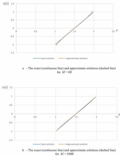
The regularizing Lavrentiev method (Kabanikhin & Shishlenin, 2019; Temirbekova & Dairbaeva, 2013) is used for the numerical solution of problems (2). The discretization was carried out with a uniform step $h=(b-a)/M$ and $x_i=a+(i-0.5)h,s_j=a+(j-0.5)h,(i,j=\overline{1,M})$, where $M$ is the number of points splitting the interval $[a,b]$. When testing the proposed approach, the regularizing parameter was chosen equal to $\mu =0.004$, ${\alpha }_k(x)=sin\frac{\pi k(2x-(b+a))}{b-a},k=1,2,\dots ,n$, the maximum number of grid nodes was 1000, the number of basis functions $n=50$, the solution was calculated with an accuracy of ${10}^{-4}$ which required from 90 to 100 thousand iterations. The absolute error between the exact and calculated solutions did not exceed 0.03, and the relative error was 3%.

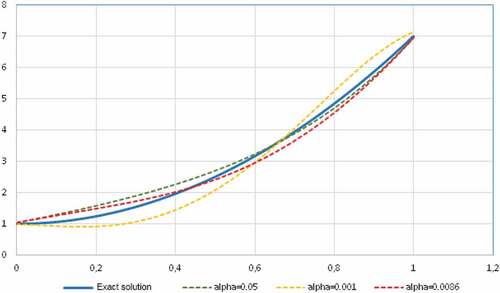
Example 2. The following example with a kernel

$K(x,s)=x^2+s$

and the right-hand side $f(x)=2+3x^2$ is considered to test the program of the Tikhonov regularization method. The exact solution of the problem is as follows:

$y(s)=1+6s^2$

.

The following parameters were chosen in the numerical calculations: $n=50,l=50,a=0,b=1,c=0,d=1,$$\xi =0÷{10}^{-6},{\delta }_f=0\cdot {10}^{-6},{\alpha }_1=4,{\alpha }_m=4\cdot {10}^{-4},\theta ={10}^{-\frac{4}{9}}$.

Here $m=10,{\alpha }_m=4\cdot {10}^{-4}$. The parameter $\mathrm{\aleph }({\alpha }_i)$ varied from $\mathrm{\aleph }({\alpha }_1)=0.429208$ to $\mathrm{\aleph }({\alpha }_8)=0.004837$ and $\mathrm{\aleph }({\alpha }_9)=-0.29\cdot {10}^{-10}$. Therefore, ${\alpha }_d=0.00111302$, $\sqrt{{\beta }_{{\alpha }_d}}=0.02208$,$\sqrt{{\beta }_{{\alpha }_d}}/{∥\tilde{f}∥}_{L_2}=0.00705,$$\mu =0.00048774$, ${∥y_{{\alpha }_d}∥}_{L_2}=3.56539$, ${\mathrm{\Phi }}_{{\alpha }_d}[y_{{\alpha }_d},\tilde{f}]=0.01464$.

The results of the approximate and exact solutions are shown in Figure Figure 3. The results of numerous methodological calculations for various $\alpha$ in the range from 0.0008 to 0.01 are presented. It can be seen from Figure Figure 3 that the numerical solution best approaches the exact solution when the regularization parameter increases, that is $\alpha =0.05$.

Figure 3. Exact and approximate solutions of the problem for different regularization parameters.

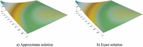
Example 3. Consider the following example (Ma et al., 2015) to perform methodological calculations using the algorithm proposed in Section 3 for solving the two-dimensional Fredholm equations of the first kind:

(63) $K(x,y,s,t)=\frac{x}{(8+y)(1+s+t)},f(x,y)=\frac{x}{6(8+y)},a=0,b=1,c=0,d=1.$(63)

A two-dimensional integral equation with a kernel and a right-hand side defined in (63) has an exact solution $V(s,t)=\frac{1}{{(1+s+t)}^2}$.

The following parameters were chosen for the numerical calculation of the two-dimensional Fredholm equation of the first kind: $\alpha =0.000001,\epsilon =0.0000001,\delta ={10}^{-7},\xi ={10}^{-7}$. The following parameters were obtained as a result of the numerical solution by the proposed algorithm: $\beta =0.000112,\mu =0.000112,\gamma =0.1159332,$$\zeta =0.0001112,\mathrm{\aleph }=0.000112$. The number of iterations was equal to 943. The calculations results are shown in Figure Figure 4.

Figure 4. Approximate and exact solutions at $n=20,m=20$.

2.5. Application for determining the distribution of lithium anomalies at depth

The described algorithm is used in calculations of the practical problem of the continuation of potential fields in the direction of disturbing masses, which is described by the Fredholm integral equation of the first kind (Tikhonov, 1999). The real data of a specific mineral deposit were used. A comparison of the results indicates a confident determination of the occurrence depth of the sources.

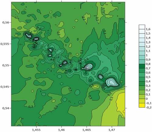
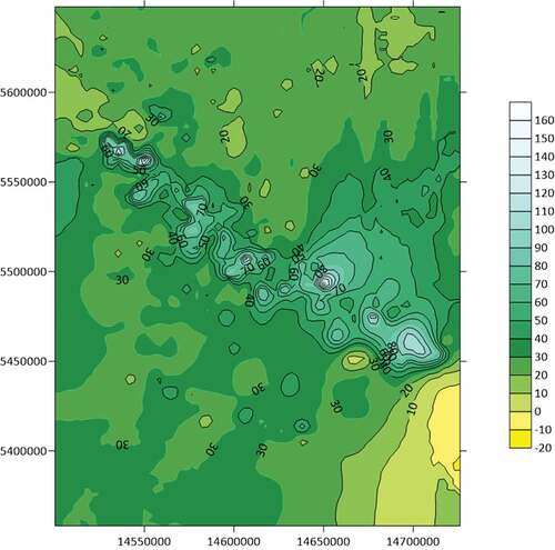
Numerical data were processed and analyzed using the mathematical methods described above and the developed software suite. The data were obtained in the engineering laboratory during analytical studies of ICP-MS spectroscopy. 777 samples were taken on 70 chemical elements in the surveyed area of more than 40 thousand square kilometers, which were obtained in expedition studies on the geochemistry and mineralogy of loose deposits of Rudny Altai and Kalba mineral deposits (Dyachkov et al., 2017). Figure Figure 5 shows the digital surface constructed using the Surfer plotting software showing the distribution of Lithium anomalies on the day surface according to the data collected during field and laboratory research. In Figure Figure 6, a digital surface is plotted in Surfer for the distribution of Lithium anomalies at depth based on the data obtained by the numerical methods proposed above and a software suite.

Figure 5. Distribution of Lithium anomalies on the day surface.

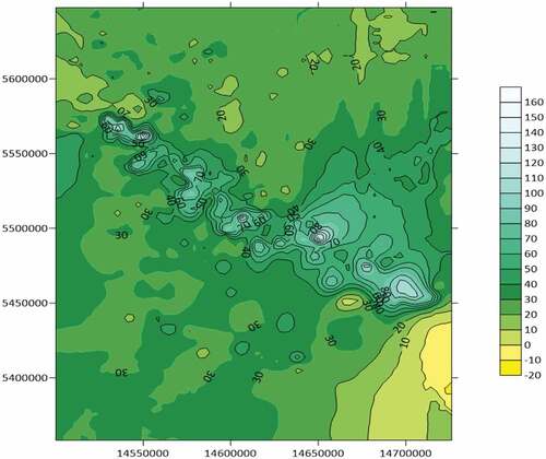
Figure 6. Nature of the distribution of Lithium anomalies at depth, numerically implemented by the proposed methods.

Real drilling data from the Kalba-Narym zone are used (Kuzmina et al., 2013) to compare the results of numerical calculations. Table 1 shows the results of the anomalous points of Lithium distribution on the surface and at a depth of 300 meters.

Table 1. Concentration of Lithium

№	Sample	Concentration on the surface	Concentration at a depth of 300 meters	The result of numerical calculations for a depth of 300 meters
1	G-71	105.8	107.7	110.2
2	G-115	132.7	128.4	130.3
3	G-169	126.6	127.8	130.4
4	G-181	133	131.5	130.8
5	G-185	141	142.3	140.7
6	G-498	104.1	107.6	110.3
7	Q-498	156.975	158.5	160.1
8	G-173	122.2	119.3	120.4

The results of the concentration comparisons showed that the discrepancy between the calculated data and the sample data from wells is about 2–4 %.

3. Conclusion

The developed methods of numerical implementation of the mathematical geophysics and geochemistry inverse problems have shown satisfactory accuracy on test examples.

In this paper, discretized Fredholm integral equations of the first kind and convergent iterative processes are considered. In principle, they can be used to find a solution to an integral equation with the replacement of the integral by a quadrature sum with an arbitrarily high accuracy, choosing sufficiently small grid steps. In this case, both the dimension of the approximate problem and the cost of solving it increase. Therefore, in numerical calculations, an increase in the accuracy of approximate solutions on a sequence of grids is used. Application of this approach allows using only known quadrature and cubature formulas in calculations. Such a statistical analysis of the number of grid nodes makes it possible to obtain an approximate solution with the required accuracy.

The developed module in the form of a software suite was used for digital modeling of a specific deposit to identify hidden ore objects. All numerical calculations were performed on a 2-processor rack server 1 U 2xS 8xDDR4 4 × 3.5/CPU 2xCLX 4214 R/DDR4 2x16GB 2933 MHZ/Net 2xSFP 10Gb, which is remotely serviced in the data center of Academset LLP, Almaty.

Acknowledgement

The work was supported by the Ministry of Education and Science of the Republic of Kazakhstan (Grant IRN AP08856012, “Development of a geoinformation system module based on methods of intelligent anomalies detection for deep field surveys”, 2020-2022).

Disclosure statement

No potential conflict of interest was reported by the author(s).

Additional information

Funding

This work was supported by the Ministry of Education and Science of the Republic of Kazakhstan [IRN AP08856012].

Notes on contributors

Nurlan Temirbekov

Temirbekov N. M., Dr. Phys. Math. Sc., Professor, corresponding member of NAS RK, academician of NEA RK. H-index is 3. According to the results of scientific research, 2 monographs and more than 100 scientific articles have been published. He is engaged in research of well-posedness of mathematical models of nonlinear physical processes, development of difference schemes and effective numerical algorithms. He led research projects in the field of mathematical modeling and information systems. The rich and successful experience of the project supervisor allows conducting mathematical justification of the well-posedness of mathematical models, effectively implement numerical methods for solving problems and create complexes of computer applications.

A GIS module is developing in this project based on intelligent anomaly detection methods for deep predictive and search modeling of hidden deposits. Construction of a complex forecast-mineragenic model consisting of a geochemical and geophysical part and digital modeling by methods of inverse problems of geochemistry and geophysics.

References

- Bahmanpour, M, Kajani, M.T., & Maleki, M. (2019). Solving Fredholm integral equations of the first kind using Muntz wavelets. Applied Numerical Vathematics, 143, 159–21. https://doi.org/10.1016/j.apnum.2019.04.007
- Daugavet, I. K. The theory of approximate methods. Linear equations. – 2 Revised and enlarged (St. Petersburg: BHV – Peterburg), 2006. 288 p. (in Russian).
- Didgar, M., Vahidi, A., & Biazar, J. (2019). A pplication of Taylor expansion for fredholm integral equations of the first kind. Journal of Mathematics, 51(5), 1–14.
- Dmitriev, V. I. (2017). On the two-dimensional inverse problem of magnetotelluric sounding of an inhomogeneous medium. Applied Mathematics and Computer Science, 56: 5–17 https://cs.msu.ru/sites/cmc/files/docs/dmitriev_22.pdf. (in Russian).
- Dyachkov, B. A., Gavrilenko, O. D., & Bubniak, A. N. (2017). Current state and problems of regional geological study of the territory of East Kazakhstan. Geology and Subsurface Protection, 3 (64), 31–37 https://elibrary.ru/item.asp?id=32327588 . in Russian
- Hosseinzadeh, H., Dehghan, M., & Sedaghatjoo, Z. (2020). The stability study of numerical solution of Fredholm integral equations of the first kind with emphasis on its application in boundary elements method. Applied Numerical Mathematics, 158, 134–151. https://doi.org/10.1016/j.apnum.2020.07.011
- Kabanikhin, S. I., & Shishlenin, M. A. (2019). Theory and numerical methods for solving inverse and ill-posed problems. Journal of Inverse and Ill-Posed Problems, 27(3), 453–456. https://doi.org/10.1515/jiip-2019-5001
- Kochnev, А. P., & Yurenkov, Y. G. Basics of predictive search models typing. . 2014. No. 1 44 ( 44). P. 74–80 (in Russian).
- Kuzmina, O. N., Dyachkov, B. A., Vladimirov, A. G., Kirillov, M. B., & Redin, Y. O. (2013). Geology and mineralogy of the gold-bearing periods of East Kazakhstan. Geology and Geophysics, 54 (12), 1889–1904 . in Russian
- Ma, Y., Huang, J., & Li, H. (2015). A novel numerical method of two-dimensional Fredholm integral equations of the second kind. Mathematical Problems in Engineering, 2015(ID 624013), 9. https://doi.org/10.1155/2015/625013
- Magnetotelluric sensing method 2005 . URL:http://nw-geo.ru/geophysics/tech/amt/
- Maleknejad, K., & Saeedipoor, E. (2017). An efficient based on hybrid functions for Fredholm integral equation of the first kind with convergence analysis. Applied Mathematics and Computation, 304, 93–102. http://dx.doi.org/10.1016/j.amc.2017.01.013
- Marchuk, G. I. Conjugate equations and their applications // Proceedings of the institute of mathematics and mechanics N.N. Krasovskii Institute of Mathematics and Mechanics, Ekaterinburg, Ural Branch of the Russian Academy of Sciences, 2006, Vol. 12, No. 1, P. 184–195 (in Russian).
- Mohammad, M., & Cattani, C. (2020). A collocation method via the quasi-affine biorthogonal systems for solving weakly singular type of Volterra-Fredholm integral equations. Alexandria Engineering Journal, 59(4), 2181–2191. https://doi.org/10.1016/j.aej.2020.01.046
- Mohammad, M., & Trounev, A. (2020). Fractional nonlinear Volterra-Fredholm integral equations involving Atangana-Baleanu fractional derivative: Framelet applications. Advances in Difference Equations, 2020(1), 618. https://doi.org/10.1186/s13662-020-03042-9
- Mohammad, M. (2019). A numerical solution of Fredholm integral equations of the second kimd based on tight framelets generated by the oblique extension principle. Journal Symmetry, 11(7), 854. https://doi.org/10.3390/sym11070854
- Shiri, B., Guo-Cheng, W., & Baleanu, D. (2020). Collocation methods for terminal value problems of tempered fractional differential equations. Applied Numerical Mathematics, 156, 385–395. https://doi.org/10.1016/j.apnum.2020.05.007
- Shiri, B., Perfilieva, I., & Alijani, Z. (2021). Classical approximation for fuzzy Fredholm integral equation. Fuzzy Sets and Systems, 404, 159–177. https://doi.org/10.1016/j.fss.2020.03.023
- Shokin, Y. I., & Potapov, V. P. (2015). GIS today: Status, prospects, solutions. Computing technologies, 20(5), 175–213. (in Russian).
- Spichak, V. V. (2005). Methodology of neural network inversion of geophysical data. Earth Physics, 3: 71–85. (in Russian).
- Temirbekova, L. N. Processing of big data in the detection of geochemical anomalies of rare-earth metal deposits. AIP conference proceeding 4th International Conference on Analysis and Applied Mathematics, ICAAM 2018; Mersin 10; Turkey; 6 September 2018 до 9 September 2018;. 2018. Vol. 1997, No. 020072 doi:10.1063/1.5049066.
- Temirbekova, L. N., & Dairbaeva, G. (2013). Gradient and direct method of solving Gelfand-Levitan integral equation. Applied and Computational Mathematics, 12(2), 234–246 .
- Tikhonov, A. N. , 1999 Mathematical Geophysics. (Moscow: Joint Institute of Earth Physics, Russian Academy of Sciences) . 476 p. (in Russian)
- Verlan, A. F., & Sizikov, V. S. . . Integral equations: methods, algorithms, programs. Reference manual. (Kiev: Naukova Dumka), 1986, 537 p. (in Russian).
- Yuan, D., Lu, S., Li, D., & Zhang, X. (2019). Graph refining via iterative regularization framework. SN Applied Sciences, 1(387), 1–10. https://doi.org/10.1007/s42452-019-0412-9
- Yuan, D., & Zhang, X. (2019). An overview of numerical methods for the first kind Fredholm integral equation. SN Applied Sciences, 1(1178), 1–12. https://doi.org/10.1007/s42452-019-1228-3