Dynamic analysis and frequency response of cylindrical roller bearing of an airflow root blower

Abstract

Cylindrical roller bearing is an important component of the airflow root blower of a power generation plant, and its malfunction has been identified as one of the root causes of poor quality demineralized water produced during operation. Hence, there is need to study the dynamic behaviour of a typical cylindrical roller bearing of an airflow root blower. In this study, the dynamic analysis of a cylindrical roller bearing subjected to different rotational speeds was simulated using finite element analysis software, Abaqus. The frequency response of the bearing was determined experimentally and analytically, and the modal frequency results obtained from both analyses were compared. The outcome of the dynamic analysis showed that the maximum temperature and Hertzian stress was developed on the outer ring of the bearing during operation, thus making this component most prone to failure. It was observed that the value of the temperature and stress developed increase with an increase in rotational speed. However, at a rotational speed greater than 503 rad/s, a drop in the Hertzian stress was developed due to the stress relaxation the bearing experience at the higher temperatures. A good agreement was obtained when the modal frequency of the frequency response obtained numerically was compared with those obtained experimentally.

Keywords:

• Abaqus
• inner ring
• Hertzian stress
• friction
• modal frequency
• failure

PUBLIC INTEREST STATEMENT

The unplanned failure of the airflow root blower of power generation plants has resulted in the production of low-quality demineralised water. The low-quality demineralised water produced as a result of failed airflow root blower is known to affect the smooth running of power generation plants. A preliminary study conducted on the airflow root blower identified the cylindrical roller bearing as the root cause of the early and unplanned failure experienced in the bower. Hence, the need to simulate the dynamic behaviour of a typical cylindrical roller bearing of an airflow root blower subjected to diverse operating speeds to identify the component of the bearing that is most prone to failure and the operating speed that results in the development of the highest Hertzian stress.

1. Introduction

Roller bearings are used widely in rotating machinery (Sharma et al., 2018), and they are very an important component of the airflow root blower used in power generation companies. The unplanned failure of these bearings during operation has often resulted in the production and transportation of low-quality demineralized water, and in some cases, it has resulted in the total shutdown of the entire plant. Because roller bearings are exposed to cyclic loading during operation, their engineering failure due to different reasons is inevitable. Among these reasons is the working condition of the bearing, developed defect during fabrication, Hertzian stress developed during operation, heat generated, and vibration experienced during operation. Localised faults such as dents, spalls, pits, and scratches and faults like cage run-out, waviness, and off-size rolling elements are reasons for failure in roller bearing (Sharma et al., 2019, 2020).

The roller bearings used in machinery come in different types such as cylindrical roller bearing, spherical roller bearing, tapered roller bearing, thrust bearing, etc. An airflow root blowers being one of such machines that operate in a compression range of 1.1–1.2 (Verma, 2014) and are used to discharge compressed air/demineralized water into a mechanical system at a steady flow rate, depending on the system requirement, it uses a cylindrical roller because the bearing has a high load-bearing capacity, and it is capable of operating efficiently under moderate speed and heavy-duty applications (Sehgal et al., 2000; Upadhyay et al., 2013; Sharma et al., 2014, 2015).

Under normal operating conditions of bearings, the bearing geometry optimisation and the design of its clearances are executed via static analysis or through modification with different measurements (Qian & Jacobs, 2014). Lately, this route is faced with a severe bottleneck, and the solution to these problems is far from being found because of the lack of information on the behaviour of the bearings under different operating speeds or transient cases. Also, it is uneconomical and, most times, unrealistic to build a test rig capable of obtaining in details the contact forces of the roller-raceway, roller-cage pocket, and the slippage of the cage and roller (Qian & Jacobs, 2014), as these are paramount in the determination of the dynamic behaviour of the bearing during operation.

The modelling of the dynamic behaviour of rolling bearing comprising localize defects on the outer and inner raceway surface has been greatly investigated by different researchers. Among the several studies reported, Mcfadden and Smith (1984) developed the pulse sequence model for investigating the vibration behaviour of a rolling bearing comprising single-point defect. In their model, a periodic impulse force with Dirac function was incorporated such that the model shows the vibration pattern generated from a rolling bearing with a single point defect when a constant load is applied. In a similar study, Su and Lin (1992) developed a pulse sequence model capable of investigating the vibration response of groove ball bearings containing single-point defect on their surfaces, under a specified time, using different loads. In the quest to obtain good results, Petersen et al. (2015) developed 2-DOF dynamic model, putting into consideration the stiffness that could occur from the effect of varied time and load distribution on the bending vibration frequency of ring bearings. Additionally, a multibody dynamic model of a cylindrical bearing (comprising localized defect) was developed by Wang et al. (2015) for the investigation of vibration responses of defect.

Several other models have been reported in literature establishing different ways to investigate the vibration responses of bearings and focusing on the effect of the localized defect (Kang et al., 2019; Niu et al., 2016, 2015; Yan et al., 2020 Hlebanja et al., 2019). Amongst these, the resonance demodulation technology has been recognized as a viable signal processing method that could be utilized to diagnose mechanical faults, especially the fault in rolling bearing (Wu & Zhang, 2016). Although, this process has a few weaknesses that have limited its applications. To circumvent the limitations encountered in utilizing the resonance demodulation method, recent studies (Dulinska & Szczerba, 2013; Jovanović & Tomović, 2014; Patra et al., 2019) now focus on the dynamic analysis of bearings, especially the non-linear dynamic behaviour of high speed and minor faults in bearing using new methods.

In this study, both experimental and finite element (FE) techniques were employed to determine the dynamic behaviour of the cylindrical roller bearing of an airflow root blower when subjected to different operating speeds. For the experimental analysis, CoCo-80 meter analyser was used to determine the frequency response of the bearing, while finite element analysis (FEA) software, Abaqus was used to compute the dynamic behaviour of the bearing under the different rotational speeds considered.

2. Dynamic loading and heat generation in bearings

Roller bearings in airflow root blower or other engineering machinery are often subjected to dynamic loading during service. When this occurs, the contact between the components of the bearing as they slide past one another leads to heat generation. The expression for the dynamic loading of a roller bearing and the heat generated in the components of roller bearing of an airflow root blower or any other engineering machinery are presented in this section.

2.1. Loading of bearings

If the size of the bearing used in a mechanical component such as the airflow root blower is determined by other factors aside from the load, the size and load-carrying capacity form the basis for loading such bearing. Furthermore, fatigue failure is less prevalent in such bearing if a very light load is applied, but raceways smearing or skidding and cage damage tends to be the dominant mechanism of failure. If very light loads are applied on a bearing, failure due to fatigue becomes less prevalent, while raceways skidding or smearing and cage damage appear to be the dominant failure mechanisms. Thus, to attain a satisfactory operation, a minimum load must be applied to the bearing. When a bearing has spherical balls, it must be subjected to a minimum load P_m = 0.01 C, and if the balls of the bearing are cylindrical, the minimum load it must be subjected to is P_m = 0.02 C.

where C is the basic static load rating (kN).

2.2. Lifespan of bearing

The accurate estimation of the useful life component is very crucial in the determination of when such component can be replaced when it is subjected to operation. For a roller bearing, the number of cycles or hours of operation prior to failure due to fatigue can be determined if the equivalent dynamic radial loading the bearing is subjected to is known. This load account for the axial and radial stresses developed in the bearing during operation. If a cylindrical roller bearing is subjected to a simultaneous axial load (${\mathrm{F}}_{\mathrm{a}}$) and a radial load (${\mathrm{F}}_{\mathrm{r}}$) having a fixed magnitude and direction, the equivalent dynamic load P can be computed as follow:

(1) $\mathrm{P}=\mathrm{X}{\mathrm{F}}_{\mathrm{r}}+\mathrm{Y}{\mathrm{F}}_{\mathrm{a}}$(1)

where P is the equivalent dynamic load (kN), ${\mathrm{F}}_{\mathrm{a}}$ is the axial load (kN), ${\mathrm{F}}_{\mathrm{r}}$ is the radial load in (kN), and $\mathbf{X}$ and $\mathbf{Y}$ represent the radial and axial loading factor, respectively.

For bearings that allow axial loads only, the dynamic load is simplified such that the load acts centrically and the equivalent dynamic load is expressed as:

(2) $\mathrm{P}={\mathrm{F}}_{\mathrm{a}}$(2)

2.3. Analysis of bearing motion

If a roller bearing radially loaded such that the inner ring rotates at an angular velocity ${\omega }_{\mathrm{i}}$, thereby causing the cylindrical balls and cage to rotate about the axis of rotation at an angular velocity ${\omega }_{\mathrm{c}}$ while the cylindrical balls revolve along their axis at an angular velocity ${\omega }_{\mathrm{r}}$.

Roller bearings used often in low-speed and heavy load applications, and the relationship between roller-raceway of such bearing is presumed to be pure rolling because the skid between the raceways and rollers are usually negligible (Deng et al., 2014; Ma et al., 2016). Hence, the average linear velocity of the roller-inner raceway and roller-outer raceway can be expressed as (Ma et al., 2016):

(3) ${\mathrm{U}}_{\mathrm{i}}=0.5{\mathrm{d}}_{\mathrm{m}}\left[\left(1-\gamma \right)\left({\omega }_{\mathrm{i}}-{\omega }_{\mathrm{c}}\right)+\left(\mathrm{D}/{\mathrm{d}}_{\mathrm{m}}\right){\omega }_{\mathrm{r}}\right]$(3)

(4) ${\mathrm{U}}_{\mathrm{o}}=0.5{\mathrm{d}}_{\mathrm{m}}\left[\left(1+\gamma \right){\omega }_{\mathrm{c}}+\left(\mathrm{D}/{\mathrm{d}}_{\mathrm{m}}\right){\omega }_{\mathrm{r}}\right]$(4)

where ${\mathrm{d}}_{\mathrm{m}}$ is the roller pitch diameter, $\mathrm{D}$ is the diameter of the roller,$\gamma =\frac{\mathrm{D}}{{\mathrm{d}}_{\mathrm{m}}}cos\alpha$, ${\omega }_{\mathrm{i}}$ is the angular velocity (rad/s) of the inner and outer ring, ${\omega }_{\mathrm{c}}$ is the cage’s angular velocity (rad/s), ${\omega }_{\mathrm{r}}$ is the angular velocity (rad/s) of the roller about its axis, ${\mathrm{U}}_{\mathrm{i}}$ is the average linear velocity of the inner roller-runway, and ${\mathrm{U}}_{\mathrm{o}}$ is the average linear velocity of the outer roller-runway.

2.4. Heat generation in roller bearing

The cage of roller bearings ride of the outer surface of the inner ring such a force ${\mathrm{F}}_{\mathrm{C}\mathrm{S}}$ is formed between the surfaces. Using Petroff’s law (Harris & Kotzalas, 2006), the force ${\mathrm{F}}_{\mathrm{C}\mathrm{S}}$ and the heat generated ${\mathrm{H}}_{\mathrm{C}\mathrm{S}}$ as a result of the frictional effect between the two surfaces can be computed as follow:

(5) ${\mathrm{F}}_{\mathrm{C}\mathrm{S}}=\frac{2\pi \phi {\mathrm{b}}_{\mathrm{c}}{\mathrm{r}}_{\mathrm{c}}^2\left({\omega }_{\mathrm{i}}-{\omega }_{\mathrm{c}}\right)}{{\delta }_{\mathrm{c}}}$(5)

(6) ${\mathrm{H}}_{\mathrm{C}\mathrm{S}}=0.5{\mathrm{d}}_{\mathrm{m}}{\mathrm{F}}_{\mathrm{C}\mathrm{S}}\left({\omega }_{\mathrm{i}}-{\omega }_{\mathrm{c}}\right)$(6)

2.5. Heat generation due to roller-cage pocket contact

The developed frictional force, ${\mathrm{F}}_{\mathrm{P}}$, resulting from the roller-cage pocket contact is expressed as (Pouly et al., 2010)

(7) ${\mathrm{F}}_{\mathrm{P}}=\frac{2\pi \phi {\mathrm{l}}_{\mathrm{P}}{\mathrm{b}}_{\mathrm{p}}^2{\omega }_{\mathrm{r}}}{{\delta }_{\mathrm{P}}}$(7)

For $Z$ roller-cage pocket contacts, the total heat generation rate is expressed as

(8) ${\mathrm{H}}_{\mathrm{P}}=\mathrm{Z}\mathrm{D}{\mathrm{F}}_{\mathrm{P}}{\omega }_{\mathrm{r}}$(8)

where $Z$ is the number of rollers, ${\mathrm{l}}_{\mathrm{P}}$ is the cage pocket axial length, $\phi$ is the dynamic viscosity of the lubricant oil, ${\mathrm{b}}_{\mathrm{P}}$ is the width of elliptic point contact, and the clearance of the roller and cage is represented with ${\delta }_{\mathrm{P}}$.

2.6. Heat generated by roller churning

The exerted drag force on a roller in the presence of lubricant and air when the roller rotates around a shaft leads to the generation of heat, and the generated heat can be expressed as follow (Deng et al., 2014):

(9) ${\mathrm{F}}_{\mathrm{d}}=\frac{1}{8}{\mathrm{C}}_{\mathrm{d}}\rho \mathrm{D}{\mathrm{l}}_{\mathrm{e}}{\left({\mathrm{d}}_{\mathrm{m}}{\omega }_{\mathrm{c}}\right)}^2$(9)

where ${\mathrm{C}}_{\mathrm{d}}$ is the drag force coefficient of the roller, ${\mathrm{d}}_{\mathrm{m}}$ is the mass density of the lubricant and air mixture in the housing, ${\mathrm{F}}_{\mathrm{d}}$ is the drag force (N), and ${\mathrm{l}}_{\mathrm{e}}$ is the effective length of the roller.

Hence, the total heat ${\mathrm{H}}_{\mathrm{d}}$, generated in Z roller churning is expressed as:

(10) ${\mathrm{H}}_{\mathrm{d}}=0.5\mathrm{Z}{\mathrm{F}}_{\mathrm{d}}{\mathrm{d}}_{\mathrm{m}}{\omega }_{\mathrm{c}}$(10)

2.7. Heat generation due to roller-raceway contact

The total heat generated ${\mathrm{H}}_{\mathrm{R}\mathrm{R}}$ as a result of the roller-raceway contact can be obtained by integrating the product of the slicing linear velocity of the roller and the lubricating shear velocity of the roller-raceway (Ma et al., 2016; Wang, 2013).

2.8. Total heat generated in roller bearing

Since a roller bearing comprises of a cage, rollers/cylindrical balls, and inner and outer ring, the total generated heat in the entire bearing can be computed as follow..

(11) ${\mathrm{H}}_{\mathrm{T}\mathrm{o}\mathrm{t}}={\mathrm{H}}_{\mathrm{d}}+{\mathrm{H}}_{\mathrm{C}\mathrm{S}}+{\mathrm{H}}_{\mathrm{P}}+{\mathrm{H}}_{\mathrm{R}\mathrm{R}}$(11)

2.9. Contact stress developed

If two cylindrical surfaces with with parallel axis and radii $R_A$ and $R_B$, are in contact, as shown in Figure 1, the developed Hertzian stress or contact pressure can be determined as follows (Adman & Yusof, 2020; Chula, 2017; Zhu, 2012):

Figure 1. Contact between two cylindrical surfaces (Chula, 2017).

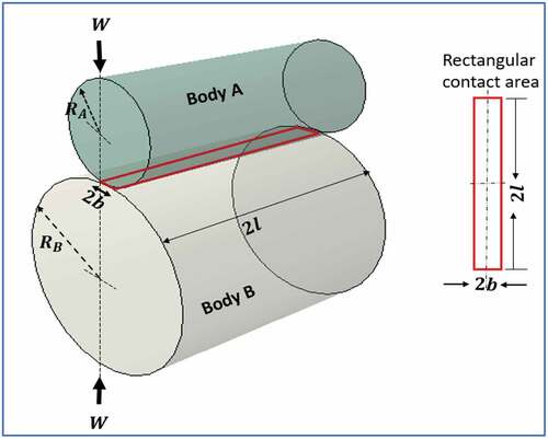
The reduced radius ($R{ }^{\mathrm{\prime }}$) of the two surfaces in contact is calculated, as shown below:

(12) $\frac{1}{R{ }^{\mathrm{\prime }}}=\frac{1}{R_A}+\frac{1}{R_B}$(12)

while the reduced Young’s modulus of elasticity ($E{ }^{\mathrm{\prime }}$) is computed as:

(13) $\frac{1}{E{ }^{\mathrm{\prime }}}=\frac{1}{2}\left[\frac{1-v_A^2}{E_A}+\frac{1-v_B^2}{E_B}\right]$(13)

Also, Equation (14)(14) $b=\sqrt{\left(\frac{4WR{ }^{\mathrm{\prime }}}{\pi lE{ }^{\mathrm{\prime }}}\right)}$(14) can be used for calculating the width of the contact area of the surfaces:

(14) $b=\sqrt{\left(\frac{4WR{ }^{\mathrm{\prime }}}{\pi lE{ }^{\mathrm{\prime }}}\right)}$(14)

Hence, the maximum pressure developed on the two surfaces when in contact can be determined using Equation (15)(15) $P_{Max}=\frac{W}{\pi bl}$(15) :

(15) $P_{Max}=\frac{W}{\pi bl}$(15)

while the developed Hertzian stress resulting from the contact between the cylindrical surfaces is computed as follow:

(16) $\sigma =0.304P_{Max}\times Z$(16)

where $R{ }^{\mathrm{\prime }}isthe$ reduced radius, $E{ }^{\mathrm{\prime }}$ is the reduced Young modulus (Pa), $R_A$ and $R_B$ are the radius of cylinder A and B, respectively, in (m), $E_A$ and $E_B$ are the Young modulus of cylinder A and B, respectively, in (Pa), $v_A$ and $v_B$ are the Poisson ratio of cylinder A and B, respectively, $b$ is the with of the surfaces in contact, $W$ is normal applied load (N), $l$ is length of contact or the height of the cylinder roller (m), $Z$ is the number of cylindrical rollers, $P_{Max}$ is the maximum contact pressure (Pa), and $\sigma$ is the Hertzian stress developed due to the contacts between the rotating surfaces.

2.10. Frequency response analysis

The structural response of components subjected to steady-state oscillatory excitation can be computed using the frequency response analysis. To conduct this analysis, an explicit definition of the excitation in the frequency domain is needed, and the excitation is applied in the form of force or enforced motions like displacements, accelerations, or velocities (Autodesk, 2018). This frequency response analysis is of two types, direct and modal frequency response.

The direct frequency response starts with the generalized equation of motion but assumes that the load is oscillating, as shown in Equation 17(17) $[\mathrm{M}]\ddot{X}(\mathrm{t})+[\mathrm{B}]\ddot{X}(\mathrm{t})+[\mathrm{K}]\mathrm{X}(\mathrm{t})=[\mathrm{F}(\mathrm{t})]$(17) .

(17) $[\mathrm{M}]\ddot{X}(\mathrm{t})+[\mathrm{B}]\ddot{X}(\mathrm{t})+[\mathrm{K}]\mathrm{X}(\mathrm{t})=[\mathrm{F}(\mathrm{t})]$(17)

where $\left[\mathrm{M}\right]$ represents the mass matrix, $\mathrm{F}\left(\mathrm{t}\right)$ represents the force vector as a function of time, $\left[\mathrm{B}\right]$ represents the damping matrix, $\left[\mathrm{K}\right]$ represents the stiffness, $(\mathrm{t})$ represents the speed, and $\stackrel{\left(\mathrm{t}\right)}{\mathrm{X}}$ represents acceleration.

To run a modal frequency response, the physical coordinates must be transformed to the modal coordinates, and a good way to do this is through the natural frequencies and eigenvectors, owning to their orthogonality properties (Autodesk, 2018).

When the solution is proposed to be in the form of an oscillating function:

(18) $X\left(t\right)=\left\{U\left(\omega \right)\right\}{e}^{i\omega t}$(18)

where, $U\left(\omega \right)$ is a complex displacement vector.

Upon taking the derivatives of the above expression, the velocity and acceleration are obtained as follow:

(19) $\dot{X}\left(t\right)=i\omega \left\{U\left(\omega \right)\right\}{e}^{i\omega t}$(19)

(20) $\stackrel{\left(t\right)}{\hspace{0.17em}X}=-{\omega }^2\left\{U\left(\omega \right)\right\}{e}^{i\omega t}$(20)

Substituting the expression for the velocity and acceleration into the equation of motion and then divide by the term $e^{i\omega t}$, we have:

(21) $-\left({\omega }^2\left[M\right]+i\omega \left[B\right]+\left[K\right]\right)\left\{u\left(\omega \right)\right\}=\left\{F\left(\omega \right)\right\}$(21)

Because the frequency $\omega$ is constant in the equation, a complex displacement vector solution would be yielded for each selected frequency.

It is important to transform physical coordinates to modal coordinates when conducting modal frequency response. One of the ways of doing this is through the eigenvectors and natural frequencies due to their orthogonal property, which allows physical coordinates $U$ to be replaced with modal coordinates to give the first transformation, as shown below:

(22) $\left\{X\right\}=\left[\mathrm{\varnothing }\right]\xi \left\{\left(\omega \right)\right\}{e}^{i\omega t}$(22)

Substituting the above equation into the equation of motion (Equation 21(21) $-\left({\omega }^2\left[M\right]+i\omega \left[B\right]+\left[K\right]\right)\left\{u\left(\omega \right)\right\}=\left\{F\left(\omega \right)\right\}$(21) ) and temporarily ignoring the damping term, we have:

(23) $-{\omega }^2\left[M\right]\left[\mathrm{\varnothing }\right]\left\{\xi \left(\omega \right)\right\}+\left[K\right]\left[\mathrm{\varnothing }\right]\left\{\xi \left(\omega \right)\right\}=\left\{F\left(\omega \right)\right\}$(23)

Multiplying throughout by ${\left[\mathrm{\varnothing }\right]}^T$, we have:

(24) $-{\omega }^2{\left[\mathrm{\varnothing }\right]}^T\left[M\right]\left\{\xi \left(\omega \right)\right\}+{\left[\mathrm{\varnothing }\right]}^T\left[K\right]\left\{\xi \left(\omega \right)\right\}={\left[\mathrm{\varnothing }\right]}^T\left\{F\left(\omega \right)\right\}$(24)

where,

${\left[\mathrm{\varnothing }\right]}^T\left[M\right]\left[\mathrm{\varnothing }\right]=$ modal mass matrix

${\left[\mathrm{\varnothing }\right]}^T\left[K\right]\left[\mathrm{\varnothing }\right]=$ modal stiffness matrix

${\left[\mathrm{\varnothing }\right]}^T\left\{F\left(\omega \right)\right\}=$ modal load vector

Hence,

(25) $-{\omega }^2{M}_i\left\{\xi \left(\mathrm{\varnothing }\right)\right\}+K_i\left\{\xi \left(\omega \right)\right\}=\left\{F_i\left(\omega \right)\right\}$(25)

If the modal displacements $\xi$ are known, the physical displacements can be determined from the sum of the modal displacements. This approach gives the same results as the direct approach if the modal degrees of freedom are incorporated in the transformation.

3. Experimental methodology for frequency response and modal analysis

Modal analysis is one of the important non-destructive techniques used to determine and compare the frequency response of components, as the plot of the response can be used to determine the presence of defects. In this study, coco-80 meter analysis was used to determine the frequency response of the cylindrical roller bearings of an airflow root blower, and the outcome of the analysis is the validation of the simulated frequency response.

The measurement of the roller bearing’s Frequency Response Function (FRF) was acquired under free-free boundary conditions with the help of an artificially excited impact hammer. An elastic rubber band was employed to hang the roller bearing such that a free-free boundary condition used in the FE simulations is mimicked. After which an impact hammer with a calibrated of sensitivity 22.23 mV/N and supplied by Brüel & Kjær was used to excite the roller bearing in the form of an impact force. The choice of using an impact hammer instead of a modal shaker is due to the comparative advantage it offers in terms of speed, convenience, and cost though, both approaches provide the same level of accuracy for non-complex situations (Avitabile, 2001).

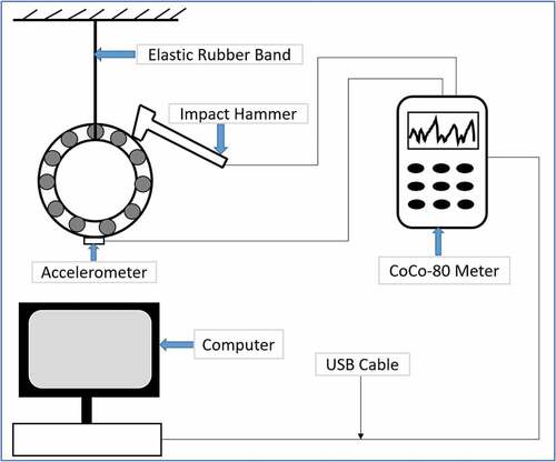
A miniature accelerometer with a sensitivity of 97.96 mV/g supplied by Brüel & Kjær and attached or fixed on the roller bearing was used for measuring the response of the bearing upon impact. After which, a 4-channel calibrated CoCo-80 meter (handheld data recorder) supplied by CRYSTAL Instruments was then used for computing the FRF measurements between input and output pairs of the roller bearing. Figure 2 shows a schematic representation of the experimental setup for conducting the modal analysis.

Figure 2. Schematic of the experimental setup.

The tip of the hammer used in impact analysis plays a major in the frequency excited, since the excitation frequency range is controlled by the hardness of the hammer’s tip selected because the harder the tip selected or used, the wider range of frequency excited by the excitation or impacted force (Avitabile, 2001). In addition, the tip of the impact hammer needs to be carefully selected so that all the required modes of vibration are excited by the impact force over the considered frequency range.

According to Avitabile (2001), the Force/Exponential window is very important in impact testing of this nature as the window minimizes leakage during the analysis, also help in forcing or shaping the data to better satisfy the FFT process periodic required by minimizing the effect of distortion caused by leakage. The exponential window is the most frequently used window when impact excitation is needed to be read on a response transducer measuring device. Hence, an exponential window was used in the CoCo-80 meter analyser to minimize/eliminate possible leakage.

This experiment was conducted under a temperature-controlled Sound and Vibration Laboratory at the Tshwane University of Technology; the following were used to perform an impact hammer test on the roller bearing:

• The roller bearing was hung on an engine crane with the aid of soft elastic rubber bands.

• An impact hammer with a metallic tip was used to apply and measure the excitation input force of the roller bearing as the bearing was repeatedly excited.

• The accelerated response at a fixed non-nodal point was measured with the aid of a miniature accelerometer attached to the roller bearing with the aid of a beeswax.

• A 4-channel CoCo-80 meter FFT analyser was used to measure the vibration signals due to the model excitation.

• The recorded FRF measured or computed by the CoCo-80 meter was extracted using the Engineering Data Management (EDM).

For this analysis, only channels 1 and 2 of four channels in the CoCo-80 meter are required. The impact hammer is connected to channel 1, while the accelerometer is connected to channel 2. Thereafter, the configuration of the impact hammer and accelerometer sensitivity is configured in the CoCo-80 meter analyser. In the configuration, the impact hammer was assigned a trigger condition such that channel 1 was assigned a High level (rising edge) to obtain the best results.

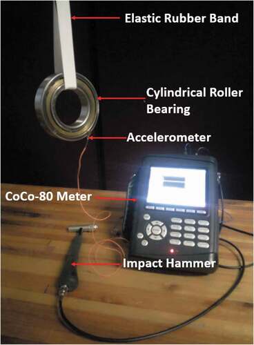
Afterwards, beeswax was subsequently used to firmly attach the miniature accelerometer (9.5 g) to one side of the roller bearing. Thereafter, one point on the roller bearing was lightly hit by the impact hammer to excite the bearing and to obtain the best frequency response functions possible. The test procedure was repeated, and the same point was impacted to obtain the best possible impact strength and to ensure repeatability of the results. Figure 3 shows an illustration of the experimental setup for conducting modal analysis of a bearing.

Figure 3. Experimental setup for frequency response analysis.

3.1. Data post-processing

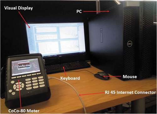
A Post-processing Engineering Data Management (EDM) software was used to identify, extract, and display experimental frequencies in waveform signals on the screen of a monitor. Thereafter, the files for the modal parameter were downloaded from the CoCo-80 meter analyser to the EDM software in an.atfx file format, and the “bode plot” signals are plotted on a graph for proper analysis of the obtained actual frequencies. The response of the roller bearing is represented in the time domain, while the response of the magnitude is presented in the frequency domain. Figure 4 shows the setup for the postprocessing of the experimental frequency response.

Figure 4. Experimental results postprocessing setup.

4. FE model analysis

To develop the model of a cylindrical roller bearing that mimics the real operating condition of the bearing of an airflow root blower of a power generation plant, finite element analysis software, Abaqus, was used. The software has the exclusive ability to model the dynamic behaviour of the bearing with a high degree of accuracy.

4.1. Development of roller bearing model

The model of the cylindrical roller bearing of an airflow root blower developed in this study using Abaqus is an assembly that consists of 1-inner ring, 1-outer ring, 1-pin-typed cage, and 13 cylindrical balls, as depicted in Figure 5. Usually, the cylindrical balls, inner and outer ring of bearings are made of the same material capable of withstanding the harsh operating condition it would be subjected to, while the cage is often made of lightweight materials since its primary function is the prevent the balls from having direct contact with one another during operation. Hence, the cage used in this study is made of Polyamide 66 (Nylon), while the cylindrical balls, inner and outer ring are made of martensitic stainless steel, X20. Table 1 shows the dimensions of the components of the cylindrical bearing of the airflow root blower developed, while the material properties of the two different materials the bearing is made of are also shown in Table 2.

Figure 5. Parts and assembly model of cylindrical roller bearing.

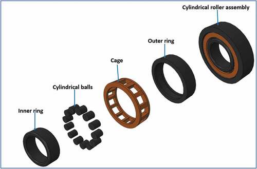
Table 1. Dimensions of cylindrical roller bearing components of an airflow root blower

Outer ring(mm)			Inner ring(mm)			Cage(mm)			Cylindrical ball (mm)
Diameter		Height	Diameter		Height	Diameter		Height	Diameter	Height
Internal	External		Internal	External		Internal	External
91.4	110.0	27.0	50.0	65.0	24.0	71.5	87.5	24.0	14.5	16.0

Table 2. Material properties of cylindrical roller bearing components of an airflow root blower (Salifu et al., 2020f, 2020e, 2020a, Hlebanja et al.)

Material properties	Polyamide (Cage)	X20 steel
Density (kg/m^3)	1 310	7 800
Elasticity (GPa)	2.95	200
Poisson’s ratio	0.41	0.28
Specific heat capacity (J/kgK)	1 680	46
Thermal expansion $\left(\times {10}^{-5}{\mathrm{K}}^{-1}\right)$	6.60	1.00
Thermal conductivity (W/m^2)	0.25	28.00

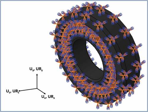
During the model development in Abaqus, appropriate coupling interaction was used to keep the components of the bearing in contact during analysis, and the assembly was assigned a general coefficient of friction with a value of 0.02. Thereafter, a dynamic explicit step was selected due to the speed associated with the analysis, and appropriate mechanical boundary conditions were defined on the bearing assembly such that displacement and rotation of the bearing during operation are possible, as shown in Figure 6. A fixed load of 160kN is thereafter applied to the inner ring after which the inner ring and the balls are subjected to four different rotational speeds 157, 300, 503, and 583 rad/s. The essence of subjecting the bearing to different operational speeds is to determine the effect of speed on the dynamic behaviour of the bearing.

Figure 6. Applied mechanical boundary conditions of cylindrical roller bearing.

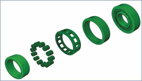
The bearing was meshed with a linear hexagonal element type C3B8T. In total, the bearing has 83 230 elements and 105 285 nodes. These elements consist of 9 734 from the outer ring, 26 688 from the polyamide cage, 5 2508 from the inner ring, while 41 600 elements were from the 13 cylindrical balls. The mesh sizes used in the study was arrived at after conducting an appropriate mesh convergence study (Salifu et al., 2019, 2020b, 2020f, 2020d, 2020c). The outcome of the study with the graph shown in Figure 7 and parts and assembly mesh depicted in Figure 8 indicate that a 2 mm inner and outer ring mesh size and a 1 mm cylindrical balls and cage mesh size are suitable for the analysis. In the determination of the suitable mesh size, the mesh size of the cage and the balls were fixed at 1 mm, while the size of the inner and outer ring being the components most prone to failure and of more interest was gradually reduced until the suitable size with reasonable computational time and degree of results accuracy were obtained.

Figure 7. Mesh convergence study plot for cylindrical roller bearing.

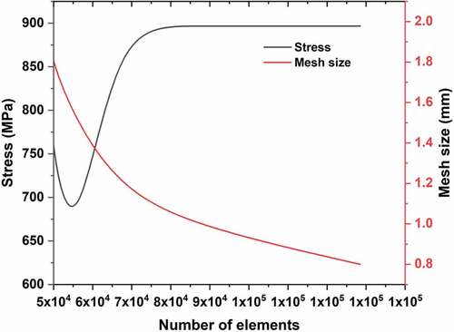
Figure 8. Parts and assembly mesh of cylindrical roller bearing.

5. Results and discussions

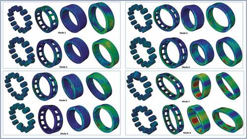
Mode shape is one of the modal parameters that allows for the visualisation of the pattern of deformation of FE model at different natural frequencies (modes of vibration). Figure 9 shows the obtained mode shapes for the first eight vibration modes. The visualisation of these mode shapes is important in understanding the dynamics of the bearing. It is worth noting that the visualization of the results of the modal stresses is used generally for the identification of hot spots or stress concentration in an FE model (Booysen, 2014). Since bending vibration modes are often expected to have the most destructive effect because of the large bending moments associated with them, and the vibration resonance of the roller bearing is greatly influenced by lower modes, only lower modes are considered in the dynamic analysis of this bearing, and the first eight mode shapes showing a symmetrically mixed pattern of the roller bearing model are shown in Figure 9.

Figure 9. Mode shape for the first eight vibration modes.

In this analysis, the eigen frequencies are extracted from the FE model of the roller bearing, and this was done without repeating any natural frequency in every mode considered due to the asymmetrical nature of the mistuned roller bearing. The FE natural frequencies for the first eight natural frequencies of the roller bearing are presented in Table 3.

Table 3. Natural frequency and mode shapes of cylindrical bearing components

Mode	Natural Frequency of Bearing (Hz)	Mode Shape
		Balls	Cage	Inner Ring	Outer Ring
1	152.6	Bend	Bend	Bend	Bend
2	301.5	Bend	Bend	Bend	Bend
3	494.7	Bend	Bend	Bend	Bend
4	711.4	Bend	Bend	Bend	Bend
5	1 034.1	Bend	Bend	Bend	Bend
6	1 551.2	Bend	Bend	Bend	Bend
7	2 326.7	Bend	Bend	Bend	Bend
8	3 490.1	Bend	Bend	Bend	Bend

5.1. Comparison of experimental and FEA modal frequency

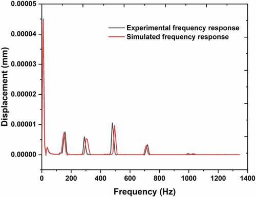
The comparison of the experimental frequency response and that obtained from the FE analysis is depicted in Figure 10. A slight deviation was observed in the amplitude and natural frequencies of the simulated and experimental response of the bearing. These slight differences between the natural frequencies could be attributed to the modelling and measurement process (Lieven & Ewins, 1988), the presence of non-linearity slight shape difference between the real and simulation models (Talai, 2016).

Figure 10. Comparison of the experimental and simulated frequency response plots.

5.2. Validation of natural frequency

In Table 4, the natural frequencies of the cylindrical roller bearing determined using FEA and experimental techniques were compared. The outcome of the comparison shown by the percentage deviation indicated that there is a strong correlation between both methods.

Table 4. Comparison of the first eight natural frequencies of cylindrical roller bearing

Mode	Natural Frequency		% Deviation
	Experimental	Simulated
1	160.0	152.6	4.63
2	290.0	301.5	3.97
3	480.0	494.7	3.06
4	720.0	711.4	1.19
5	1 000.0	1034.1	3.41

Dynamic stress analysis was conducted on the roller bearing to acquire the linearized dynamic stress distribution on the critical area of the bearing when it passes through the natural frequencies.

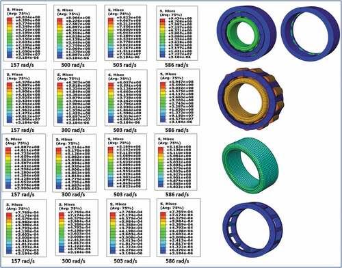
The contour plot for the temperature distribution profile obtained and the heat flux developed in the roller bearing under the different operating/rotating speeds are shown in Figures 11 and 12, respectively. From the temperature distribution plot, it was observed that the higher the operating/rotating speed, the higher the temperature developed in the bearing assembly. Based on this, the roller bearing operated at a rotational speed of 5600 RPM (586 rad/s) developed the highest temperature (216.2℃), while the roller bearing operated at a rotational speed of 1 500 RPM (157 rad/s) developed the least temperature (45.77℃). The distribution of the temperature during service across the components of the bearing for the different temperatures showed that the tip of the cylindrical balls experience the highest temperature due to its constant contact with both the inner ring and outer ring during operation, while the outer ring experiences the least thermal effect due to its fast heat loss to its surrounding. It is worth noting that the contact of the cylindrical balls with the inner and outer ring, and the characteristic high operating speed leads to friction, which consequently results in the rise in temperature, thermal expansion and stiffness of the bearing during operation (Venkatesh & Prasad, 2017).

Figure 11. Temperature distribution profile contour plot and results for the different operating speeds.

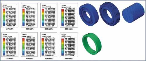
Figure 12. Results and contour plots for the distribution of heat flux for the different speeds.

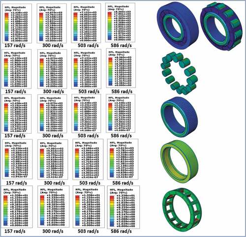
Similarly, the heat flux developed in the bearing increases with an increase in temperature. Hence, the highest heat flux was obtained in the bearing subjected to the highest operating/rotating speed. The maximum heat flux with a value of $8.56\times {10}^3\mathrm{W}/{\mathrm{m}}^2$ was developed in the bearing operated at a rotational speed of 5 600 RPM (586 rad/s), while the least heat flux with a value of $2.438\times {10}^3\mathrm{W}/{\mathrm{m}}^2$ was developed when the bearing was operated at a rotational speed of 1 500 RPM (157 rad/s). Just like the temperature distribution profile, the least heat flux was developed on the outer ring while the maximum flux was developed on the cylindrical balls.

Figure 13 shows the contour plots of the contact stress distribution profile developed on the bearing and its components for the different rotational speeds considered. From the plot, it was observed that the maximum contact/Hertzian stress, having a value of 982.3 MPa was developed in the analysis when the bearing is operated at a rotational speed of 4 800 RPM (503 rad/s). Contrary to what was experienced with the developed temperature and heat flux, where both increases with an increase in rotation speed, a reduction in the developed stress was observed when the rotational speed exceeds 4 800 RPM (503 rad/s). This reduction in the value of the stress developed in the bearing can be attributed to the stress relaxation the bearing experiences as it operates in a high-temperature regime. The least stress with a value of 682.4 MPa was developed when the rotating speed of the bearing was 1 500 RPM (157 rad/s). In all the different rotational speeds considered, the maximum Hertzian/contact stress was developed on the raceway of the outer ring (at the point of possible contact between the edge of the cylindrical ball and the outer ring). In the entire assembly, the cage made of polyamide experiences the least contact stress due to its low interference with other components of the bearing during operation. The development of maximum Hertzian stress at similar location as that obtained in this study has been reported (Kumar & Rao, 2015), though with a different maximum Hertzian stress value due to the different operating parameters used. Owing to the high contact stress developed on the outer ring of a cylindrical roller bearing, it is the most prone to failure of all the bearing’s components.

Figure 13. Contour plots and stress distribution profile results for the different operating speeds.

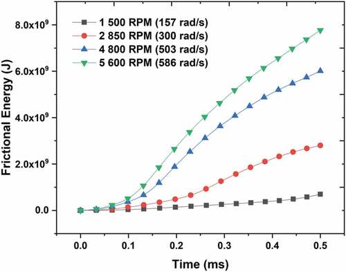
A plot of the frictional energy developed when the cylindrical bearing is subjected to the four different operational speeds is shown in Figure 14. From the plot, it was observed that the frictional energy increases with an increase in the rotational speed and operational time, such that the maximum was developed at the point of contact between the balls and the outer ring. The characteristic high frictional energy value obtained in bearings is attributed to the stiffness that occurs due to the thermal expansion in the roller bearing while in operation (Venkatesh & Prasad, 2017).

Figure 14. Fictional energy plots for the different operational speeds.

5.3. Analytical validation of Hertzian stress developed

To determine the integrity of the model developed, it is important to either validate the FEA result experimentally or analytically. In this study, Equations (12(12) $\frac{1}{R{ }^{\mathrm{\prime }}}=\frac{1}{R_A}+\frac{1}{R_B}$(12) –16(16) $\sigma =0.304P_{Max}\times Z$(16) ) were used to analytically validate the developed Hertzian stress in the bearing when it was operated at a speed of 157 rad/s and the outcome of the comparison, as depicted in Table 5, shows that there is good correlation between the analytical and FEA computed Hertzian stress results.

Table 5. Comparison of the FEA and analytically calculated Hertzian stress at 157 rad/s

Analytically computed Hertzian stress(MPa)	Simulated Hertzian stress(MPa)	% Deviation
654.9	682.4	4.20

6. Conclusion

Both FE and experimental techniques were employed in this study to determine the dynamic behaviour of an X20 fabricated cylindrical roller bearing whose pin-type cage is made of polyamide. In the experimental analysis, a non-destructive technique was used to determine the frequency response of the bearing when impacted by a hammer, while finite element analysis software was used to determine the dynamic behaviour of the bearing when subjected to different operational speeds. The modal frequencies obtained from the FEA analysis was validated using the modal results experimentally, and both results show a strong correlation.

The temperature distribution profile, heat flux, and frictional energy results obtained from the FEA showed that this parameter increases with an increase in operational speed, while the results of the Hertzian stress developed on the bearing show that the stress increases with an increase in operational speed up to 503 rad/s after which the developed stress reduces due to possible stress relaxation resulting from the high temperature developed in higher speeds. In all the operational speeds considered, the maximum Hertzian stress was developed on the raceway of the outer ring thus, making it most prone to failure of all the bearing’s components.

Acknowledgements

This work has been supported by Tshwane University of Technology and the University of Johannesburg, South Africa. Also, the authors greatly appreciate the support of Eskom Power Plant Engineering Institute (Republic of South Africa).

Disclosure statement

No potential conflict of interest was reported by the author(s).

Additional information

Funding

The authors received no direct funding for this research.

Notes on contributors

Themba Mashiyane

Engr. Themba Mashiyane is a postgraduate student at the Department of Mechanical and Mechatronics, Tshwane University of Technology, South Africa.

Prof. Dawood Desai is a seasoned researcher and senior lecturer at the Department of Mechanical and Mechatronics, Tshwane University of Technology, South Africa.

Prof. Lagouge Tartibu is a seasoned researcher and senior lecturer at the Department of Mechanical and Industrial Engineering Technology, University of Johannesburg, Johannesburg, South Africa.

References

- Adman, A. A., & Yusof, N. F. M. (2020). Analysis of contact stress and vibration of rolling element bearing. Materials Science and Engineering, 815 , 01/012001. IOP Publishing.
- Autodesk. (2018). Frequency Response Analysis Retrieved April 22, 2021, from https://knowledge.autodesk.com/support/inventor-nastran/learn-explore/caas/CloudHelp/cloudhelp/2018/ENU/NINCAD-SelfTraining/files/GUID-FCA4E4B5-1A53-480E-A43A-A208E8F3C97E-htm.html#:~:text=Modal%20Frequency%20Response%20Analysis%2C%20which,retained%2C%20reduce%20the%20problem%20size
- Avitabile, P. (2001). Experimental modal analysis. Sound and Vibration, 351, 20–22. https://classes.engineering.wustl.edu/2009/fall/mase431/PDF/modalana.pdf
- Booysen, C. (2014). Fatigue life prediction of steam turbine blades during start-up operation using probabilistic concepts. Doctoral dissertation, University of Pretoria. https://www.up.ac.za/media/shared/120/ZP_Files/Students%20presentations/public-defence-c-booysen-2014-07-25-final.zp42405.pdf
- Chula. (2017). Contact stresses. http://pioneer.netserv.chula.ac.th/~ltachai/tribology/tribo_ch07.pdf
- Deng, S. E., Jia, Q. Y., & Xue, J. X. (2014). Design principles of rolling bearings. Standards Press of China.
- Dulinska, J. M., & Szczerba, R. (2013). Simulation of dynamic behaviour of RC bridge with steel-laminated elastomeric bearings under high-energy mining tremors. Key Engineering Materials, 531, Trans Tech Publ, 662–667. https://doi.org/10.4028/www.scientific.net/KEM.531-532.662:
- Harris, T. A., & Kotzalas, M. N. (2006). Advanced concepts of bearing technology: Rolling bearing analysis. CRC press.
- Hlebanja, G., Hriberšek, M., Erjavec, M., & Kulovec, S. (2019). Durability Investigation of plastic gears. EDP Sciences. https://doi.org/10.1051/matecconf/201928702003
- Jovanović, J. D., & Tomović, R. N. (2014). Analysis of dynamic behaviour of rotor-bearing system. Proceedings of the Institution of Mechanical Engineers, Part C: Journal of Mechanical Engineering Science, United Kingdom, 228, 2141–2161. https://doi.org10.1177/0954406213516439
- Kang, J., Lu, Y., Zhang, Y., Liu, C., Li, S., & Müller, N. (2019). Investigation on the skidding dynamic response of rolling bearing with local defect under elastohydrodynamic lubrication. Mechanics & Industry, 20(6), 615. https://doi.org/10.1051/meca/2019054
- Kumar, P. M., & Rao, C. J. (2015). Structural and thermal analysis on a tapered roller bearing. IJISET-International Journal of Innovative Science, Engineering & Technology, 2(1), 502–511. http://ijiset.com/vol2/v2s1/IJISET_V2_I1_71.pdf
- Lieven, N. A. J., & Ewins, D. J. (1988). Spatial correlation of mode shapes, the coordinate modal assurance criterion (COMAC). 690–695.
- Ma, F., Li, Z., Qiu, S., Wu, B., & An, Q. (2016). Transient thermal analysis of grease-lubricated spherical roller bearings. Tribology International, 93(1), 115–123. https://doi.org/10.1016/j.triboint.2015.09.004
- Mcfadden, P., & Smith, J. (1984). Model for the vibration produced by a single point defect in a rolling element bearing. Journal of Sound and Vibration, 96(1), 69–82. https://doi.org/10.1016/0022-460X(84)90595-9
- Niu, L., Cao, H., He, Z., & Li, Y. (2015). A systematic study of ball passing frequencies based on dynamic modeling of rolling ball bearings with localized surface defects. Journal of Sound and Vibration, 357(1), 207–232. https://doi.org/10.1016/j.jsv.2015.08.002
- Niu, L., Cao, H., He, Z., & Li, Y. (2016). An investigation on the occurrence of stable cage whirl motions in ball bearings based on dynamic simulations. Tribology International, 103(1), 12–24. https://doi.org/10.1016/j.triboint.2016.06.026
- Patra, P., Saran, V. H., & Harsha, S. (2019). Non-linear dynamic response analysis of cylindrical roller bearings due to rotational speed. Proceedings of the Institution of Mechanical Engineers, Part K: Journal of Multi-body Dynamics, United Kigdom, 233, 379–390. https://doi.org/10.1177/1464419318762678
- Petersen, D., Howard, C., & Prime, Z. (2015). Varying stiffness and load distributions in defective ball bearings: Analytical formulation and application to defect size estimation. Journal of Sound and Vibration, 337(1), 284–300. https://doi.org/10.1016/j.jsv.2014.10.004
- Pouly, F., Changenet, C., Ville, F., Velex, P., & Damiens, B. (2010). Power loss predictions in high-speed rolling element bearings using thermal networks. Tribology Transactions, 53(6), 957–967. https://doi.org/10.1080/10402004.2010.512117
- Qian, W., & Jacobs, G. (2014 ()). Dynamic simulation of cylindrical roller bearings. (Doctoral dissertation, Hochschulbibliothek der Rheinisch-Westfälischen Technischen Hochschule Aachen).
- Salifu, S., Desai, D., Fameso, F., Ogunbiyi, O., Jeje, S., & Rominiyi, A. (2020a). Thermo-mechanical analysis of bolted X20 steam pipe-flange assembly. Materials Today: Proceedings. South Africa: Elsevier. https://doi.org/10.1016/j.matpr.2020.04.882
- Salifu, S., Desai, D., Kok, S., & Ogunbiyi, O. (2019). Thermo-mechanical stress simulation of unconstrained region of straight X20 steam pipe. Procedia Manufacturing, 35(1), 1330–1336. https://doi.org/10.1016/j.promfg.2019.05.021
- Salifu, S., Desai, D., & S, K. (2020b). Comparative evaluation of creep response of X20 and P91 steam piping networks in operation. The International Journal of Advanced Manufacturing Technology, 109(7–8), 1987–1996. https://doi.org/10.1007/s00170-020-05727-7
- Salifu, S., Desai, D., & S, K. (2020c). Creep–fatigue interaction of P91 steam piping subjected to typical start-up and shutdown cycles. Journal of Failure Analysis and Prevention, 20(3), 1055–1064. https://doi.org/10.1007/s11668-020-00908-8
- Salifu, S., Desai, D., & S, K. (2020d). Numerical investigation of creep-fatigue interaction of straight P91 steam pipe subjected to start-up and shutdown cycles. Materials Today: Proceedings. South Africa: Elsevier.
- Salifu, S., Desai, D., & S, K. (2020e). Numerical simulation and creep-life prediction of X20 steam piping. Materials Today: Proceedings. South Africa: Elsevier.
- Salifu, S., Desai, D., & S, K. (2020f). Prediction and comparison of creep behavior of X20 steam plant piping network with different phenomenological creep models. Journal of Materials Engineering and Performance, (11), 1–14. https://doi.org/10.1007/s11665-020-05235-5
- Sehgal, R., Gandhi, O. P., & Angra, S. (2000). Reliability evaluation and selection of rolling element bearings. Reliability Engineering & System Safety, 68(1), 39–52. https://doi.org/10.1016/S0951-8320(99)00081-2
- Sharma, A., Amarnath, M., & Kankar, P. K. (2014). Effect of varying the number of rollers on dynamics of a cylindrical roller bearing. American Society of Mechanical Engineers.
- Sharma, A., Amarnath, M., & Kankar, P. K. (2015). Effect of unbalanced rotor on the dynamics of cylindrical roller bearings. Springer.
- Sharma, A., Amarnath, M., & Kankar, P. K. (2019). Nonlinear dynamic analysis of defective rolling element bearing using Higuchi’s fractal dimension. Sādhanā, 44(1), 1–29. https://doi.org/10.1007/s12046-019-1060-x
- Sharma, A., Kankar, P. K., & Amarnath, M. (2020). Investigations on nonlinearity for health monitoring of rotor bearing system. Reliability and Risk Assessment in Engineering, (1), 241. https://books.google.co.za/books?hl=en&lr=&id=WpbiDwAAQBAJ&oi=fnd&pg=PA241&dq=Sharma,+A.,+Kankar,+P.+K.,+%26+Amarnath,+M.+(2020).+Investigations+on+nonlinearity+for+health+monitoring+of+rotor+bearing+system.+Reliability+and+Risk+Assessment+in+Engineering+1+,+241&ots=DLsJAct8Zq&sig=8P90m0n0Q4-SJFsy5TpRKnq5VPo#v=onepage&q=Sharma%2C%20A.%2C%20Kankar%2C%20P.%20K.%2C%20%26%20Amarnath%2C%20M.%20(2020).%20Investigations%20on%20nonlinearity%20for%20health%20monitoring%20of%20rotor%20bearing%20system.%20Reliability%20and%20Risk%20Assessment%20in%20Engineering%201%20%2C%20241&f=false
- Sharma, A., Upadhyay, N., Kankar, P. K., & Amarnath, M. (2018). Nonlinear dynamic investigations on rolling element bearings: A review. Advances in Mechanical Engineering, 10(3), 1687814018764148. https://doi.org/10.1177/1687814018764148
- Su, Y. T., & Lin, S. J. (1992). On initial fault detection of a tapered roller bearing: Frequency domain analysis. Journal of Sound and Vibration, 155(1), 75–84. https://doi.org/10.1016/0022-460X(92)90646-F
- Talai, S. M. (2016). Prediction of dynamic behaviour of simplified turbine blade assemblies using infrared thermography. Tshwane University of Technology.
- Upadhyay, R. K., Kumaraswamidhas, L. A., & Azam, M. S. (2013). Rolling element bearing failure analysis: A case study. Case Studies in Engineering Failure Analysis, 1(1), 15–17. https://doi.org/10.1016/j.csefa.2012.11.003
- Venkatesh, K., & Prasad, K. R. (2017). Finite element solution for thermal analysis of NiTiNOL-60. Ball Bearing.
- Verma, S. K. (2014). Numerical investigation on the performance of roots blower varying rotor profile [ Doctoral dissertation].
- Wang, F., Jing, M., Yi, J., Dong, G., Liu, H., & Ji, B. (2015). Dynamic modelling for vibration analysis of a cylindrical roller bearing due to localized defects on raceways. Proceedings of the Institution of Mechanical Engineers, Part K: Journal of Multi-Body Dynamics, 229, 39–64. United Kingdom: SagePub.
- Wang, L. Q. (2013). Design and numerical analysis of rolling element bearing for extreme applications. Harbin Institute of Technology Press.
- Wu, Z., & Zhang, J. C. (2016). Finite element analysis and experimental study on failure rolling bearing. Key Engineering Materials, 693(1), 332–339. Trans Tech Publ. https://doi.org/10.4028/www.scientific.net/KEM.693.332
- Yan, P., Yan, C., Wang, K., Wang, F., & Wu, L. (2020). 5-DOF dynamic modeling of rolling bearing with local defect considering comprehensive stiffness under isothermal elastohydrodynamic lubrication. Shock and Vibration, 1(1), 1–15. https://doi.org/10.1155/2020/9310278
- Zhu, X. (2012). Tutorial on hertz contact stress. OPTI, 521(1), 1–8. https://wp.optics.arizona.edu/optomech/wp-content/uploads/sites/53/2016/10/OPTI-521-Tutorial-on-Hertz-contact-stress-Xiaoyin-Zhu.pdf