
 ?Mathematical formulae have been encoded as MathML and are displayed in this HTML version using MathJax in order to improve their display. Uncheck the box to turn MathJax off. This feature requires Javascript. Click on a formula to zoom.
Abstract
In this paper, we deal with the differential properties of the scalar flux defined over a two-dimensional bounded convex domain, as a solution to the integral radiation transfer equation. Estimates for the derivatives of
near the boundary of the domain are given based on Vainikko’s regularity theorem. The optimal pointwise error estimates in terms of the scalar flux are presented for the two classic finite difference methods: diamond difference (DD) and step difference (SD). Numerical results indicate the implication of the solution smoothness on the numerical convergence behavior.
1. Introduction
The one-group radiation transfer problem in a three-dimensional (3D) convex domain reads as follows: find an angular flux function
such as
(1)
(1)
(2)
(2)
where
is the closure of the domain
with the boundary
is the unit sphere of
denotes the direction of radiation transfer,
is the extinction coefficient (or macroscopic total cross section in neutron transport),
is the scattering coefficient (or macroscopic scattering cross section),
is the phase function of scattering with
is the external source function, and
is the unit normal vector of the domain surface. Note that
under the subcritical condition, and
Assuming the isotropic scattering isotropic source
and isotropic boundary condition
we can obtain the so-called Peierls integral equation of radiation transfer for the scalar flux
as follows:
(3)
(3)
(4)
(4)
where
is the differential element of the domain surface,
is the optical path between
and
One can find detailed derivation in Vainikko (Citation1993).
For simplicity, we assume and
are constant over the domain. Then EquationEquation (3)
(3)
(3) can be simplified as
(5)
(5)
where the 3D radiation kernel is given as
(6)
(6)
The boundary integral term in the above equation can produce singularities in the solution. We omit its discussion in this paper. In other words, here we only consider the problem with the vacuum boundary condition, i.e., Thus, EquationEquation (6)
(6)
(6) can be treated as the weakly integral equation of the second kind:
(7)
(7)
where
is an open bounded domain and the kernel
is weakly singular, i.e.,
Note that
for radiation transfer. Weakly singular integral equations arise in many physical applications such as elliptic boundary problems and particle transport.
Since has a singularity at
the solution of a weakly integral equation is generally not a smooth function and its derivatives at the boundary would become unbounded from a certain order. There was extensive research on the smoothness (regularity) properties of the solutions to weakly integral equations (Mikhlin Citation1965; Mikhlin and Prossdorf Citation1986), especially those early work in neutron transport theory done in the former Soviet Union (Vladimirov Citation1963; Germogenova Citation1969). It is believed that Vladimirov first proved that the scalar flux
possesses the property
for the one-group transport problem with isotropic scattering in a bounded domain (Vladimirov Citation1963). Germogenova analyzed the local regularity of the angular flux
in a neighborhood of the discontinuity interface and obtained an estimate of the first derivative, which has the singularity near the interface (Germogenova Citation1969). Pitkäranta (Citation1980) derived a local singular resolution showing explicitly the behavior of
near the smooth portion of the boundary. Vainikko (Citation1993) introduced weighted spaces and obtained sharp estimates of pointwise derivatives near the smooth boundary for multidimensional weakly singular integral equations.
There exists some previous research work on the regularity of the integral radiation transfer solutions (Johnson and Pitkaranta Citation1983; Hennebach, Junghanns, and Vainikko Citation1995). However, the 2D kernel treated in those studies bears no physical meaning since it does not model the scattering correctly. A physically relevant 2D kernel can be found in Lewis and Miller (Citation1993). In this paper, we rederive the 2D kernel by directly integrating the 3D kernel with respect to the third dimension. We examine the differential properties of the new 2D kernel and provide estimates of pointwise derivatives of the scalar flux according to Vainikko’s regularity theorem for the weakly integral equation of the second kind.
The remainder of the paper is organized as follows. In Sect. 2, we derive the 2D kernel for the integral radiation transfer equation. We examine the derivatives of the kernel and show that they satisfy the boundedness condition of Vainikko’s regularity theorem in Sect. 3. Then the estimates of local regularity of the scalar flux near the boundary of the domain are given. In Sect. 4, we derive local estimates for the spatial discretization error in terms of the scalar flux for the two classical numerical methods, diamond difference (DD) and step difference (SD). Sect. 5 presents numerical results of DD and SD to demonstrate how the asymptotic convergence behavior of the spatial discretization error is affected by the smoothness of the exact solution. Concluding remarks are given in Sect. 6.
2. Two-dimensional radiation transfer equation
In this section, we derive the 2D integral radiation transfer equation from its 3D form, EquationEqs. (5)(5)
(5) and Equation(6)
(6)
(6) . In 3D,
and
Let
then
In a 2D domain
the solution function
only depends on
and
in Cartesian coordinates. Therefore, we only need to find the 2D radiation kernel, which can be obtained by integrating out
as follows:
(8)
(8)
To proceed, we introduce the variables and
Then we substitute
into the above equation to have
(9)
(9)
The above derivation of the 2D kernel is much simpler than the process given in Lewis and Miller (Citation1993), where the integral form is obtained by the projection of the particle flight path on the 2D plane. Note that the last integral is the first Bickley-Naylor function (Abramowitz and Stegun Citation1970; Altaç Citation2007).
Now we show that the 2D kernel has a singularity at
(i.e.,
as follows. As
is sufficiently small, we can have
and
(10)
(10)
Thus, it can be seen that becomes unbounded at
By replacing the 3D kernel as defined by EquationEquation (6)(6)
(6) with the above one, EquationEquation (5)
(5)
(5) becomes the 2D integral radiation transfer equation. Notice that the surface integral in the last term on the right-hand side of EquationEquation (5)
(5)
(5) should be replaced with a line integral in the 2D domain.
Remark 2.1.
By simply assuming a 2D scattering, Johnson and Pitkaranta derived a 2D kernel, i.e., (where
), which is however physically incorrect since the scattering is essentially a 3D phenomenon (Johnson and Pitkaranta Citation1983). Hennebach, Junghanns, and Vainikko (Citation1995) also used the same 2D kernel for analyzing the radiation transfer solutions. In addition, the integral equations in other geometries such as slab or sphere can be obtained by following the same approach, and they can be found in Bell and Glasstone (Citation1970).
Applying Banach’s fixed-point theorem, we can prove the existence and uniqueness of the solution in the 2D domain by showing that is bounded below unity as follows.
(11)
(11)
where
is the azimuthal angle. By extending the above bounded domain to the whole space, we have
(12)
(12)
Denoting EquationEquation (12)
(12)
(12) is simplified as
(13)
(13)
Notice we have changed the order of integration to solve the integral. It is apparent that for there exists a unique solution, the subcritical condition, must be satisfied.
Remark 2.2.
A similar proof can be found for the 2D kernel in terms of the Bickley-Naylor function (de Azevedo et al. Citation2018). Existence of the unique solution to the general neutron transport equation in and
has been long established in Case and Zweifel (Citation1967). Corresponding results in
for
can be found in (Agoshkov Citation1998; Latrach Citation2001; Latrach and Zeghal Citation2012; Egger and Schlottbom Citation2014).
3. Solution regularity
We first introduce Vainikko’s regularity theorem (Vainikko Citation1993), which provides a sharp characterization of singularities for the general weakly integral equation of the second kind. Then we analyze the differential properties of the 2D radiation kernel and show that the derivatives are properly bounded. Finally, Vainikko’s theorem is used to give the estimates of pointwise derivatives of the radiation transfer solution.
3.1. Vainikko’s regularity theorem
Before we state the theorem, we introduce the definition of weighted spaces
Weighted space For a
introduce a weight function
(14)
(14)
where
is an open bounded domain and
is the distance from
to the boundary
Let
and
Define the space
as the set of all
times continuously differentiable functions
such that
(15)
(15)
In other words, a times continuously differentiable function
on
belongs to
if the growth of its derivatives near the boundary can be estimated as follows:
(16)
(16)
where
is a constant. The space
equipped with the norm
is a complete Banach space.
After defining the weighted space, we introduce the smoothness assumption about the kernel in the following form: the kernel is
times continuously differentiable on
and there exists a real number
such that the estimate
(17)
(17)
where
(18)
(18)
(19)
(19)
holds for all multi-indices
and
with
Here the following usual conventions are adopted:
and
Now we present Vainikko’s theorem in characterizing the regularity properties of a solution to the weakly integral equation of the second kind (Vainikko Citation1993).
Theorem 3.1.
Let be an open bounded domain,
and let the kernel
satisfy the condition Equation(17)
(17)
(17) . If the integral Equationequation (7)
(7)
(7) has a solution,
then
Remark 3.1.
The solution does not improve its properties near the boundary remaining only in
even if
is of class
and
A proof can be found in Vainikko (Citation1993). More precisely, for any
and
(
) there are kernels
satisfying Equation(17)
(17)
(17) and such that EquationEquation (7)
(7)
(7) is uniquely solvable and, for a suitable
the normal derivatives of order
of the solution behave near
as
if
and as
for
3.2. Regularity of the radiation transfer solution
To apply the results of Theorem 3.1 to the 2D integral radiation transfer equation, we need to analyze the kernel and show that it satisfies the condition Equation(17)
(17)
(17) , i.e.,
We can simply set
without loss of generality for our problem.
(20)
(20)
Let
then
By the chain rule,
can be written as
(21)
(21)
Then we have
(22)
(22)
where
(23a)
(23a)
(23b)
(23b)
Substituting EquationEqs. (23a)(23a)
(23a) and Equation(23b)
(23b)
(23b) into Equation(22)
(22)
(22) , we obtain
(24)
(24)
Apparently, we only need to find the upper bound of which is shown as follows.
(25)
(25)
Now we need to find the bound for in the above equation, which is analyzed as follows.
(26)
(26)
Note that in the above equation, and
i.e., it is bounded. Substituting EquationEquation (26)
(26)
(26) into Equation(25)
(25)
(25) and noting that
we obtain
(27)
(27)
Finally, we conclude that the 2D radiation kernel satisfies the condition Equation(17)(17)
(17) . Therefore, by Theorem 3.1, the estimates of derivatives of the scalar flux
for radiation transfer are the same as those for the general weakly integral equation of the second kind:
(28)
(28)
It should be noted that in radiation transfer where
is the external source. If the function
is bounded, then
(Vainikko Citation1993).
Remark 3.2.
The first derivative of the solution behaves as
and becomes unbounded as approaching the boundary. The derivatives of order
behave as
for
These pointwise estimates cannot be improved by adding more strong smoothness on the data and domain boundary. Here, we only deal with the solution regularity in the normal direction near the boundary. It is noted that the tangential derivatives behave essentially better than the normal derivatives (Vainikko Citation1993). In other words, the solution is smoother (or less singular) in the tangential direction than the normal direction near the boundary. The obtained pointwise bounds on the derivatives are strong results, which imply bounds in other norms such as Sobolev norms. Golse et al. (Citation1988) studied the regularity of the mean value (with respect to velocity) of the solution of transport equations in terms of fractional Sobolev space.
Remark 3.3.
These sharp error estimates are needed to analyze numerical methods. The lack of smoothness in the exact solution could adversely affect the convergence rate of spatial discretization schemes for solving the radiation transfer equation (Madsen Citation1972; Larsen Citation1982; Wang and Ragusa Citation2009). The spatial discretization error of a numerical method can be expressed as where
is the exact solution,
is its numerical result,
is the mesh size,
is the order of accuracy, and
is the
-th derivative of the scalar flux. According to the above regularity results, we have
then
However, for any numerical methods, we would generally have
and thus the spatial convergence rate would asymptotically reduce to the first order of accuracy or even worse as the mesh is refined.
4. Error analysis of DD and SD
In this section, we present the optimal error estimates in terms of the scalar flux for the two classic numerical methods: DD and SD. The DD method is a second-order central finite difference method, while the SD method is a first-order upwind method. In the next section, numerical results of a homogeneous unit-square problem are presented for both DD and SD to show how the convergence behavior of numerical solutions are impeded by the underlying regularity of the exact transport solution. The derivation follows our previous analysis (Wang Citation2022) using the discrete maximum principle (Miller, O’Riordan, and Shishkin Citation2012; Stynes and Stynes Citation2018). Although the optimal error estimates are obtained for the 1D slab geometry, it is applicable for 2D problems since we are only concerned with the smoothness in the normal direction to the boundary in this work.
4.1. Error estimate for DD
The monoenergetic SN equation in slab geometry with the assumption of isotropic scattering and constant external neutron source is written as
(29)
(29)
where
is the neutron direction cosine with respect to the
-axis,
is the angular flux,
is the quadrature weight,
is the total macroscopic cross section,
is the macroscopic scattering cross section, and
is the external neutron source.
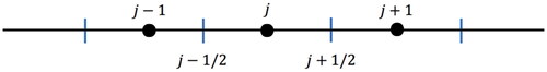
The mesh gird employed for discretizing DD and SD is shown in . The index denotes the center of cell
is the left edge, and
is the right edge.
Figure 1. One-dimensional mesh.
The DD discretization for the SN equation on the one-dimensional mesh can be written as
(30)
(30)
where
(31a)
(31a)
(31b)
(31b)
(31c)
(31c)
and
are assumed to be piecewise constant in each cell. The superscript "
" denotes the numerical solution.
We introduce the linear discrete operator for the DD discretization as
(32)
(32)
where
(33)
(33)
By multiplying with each quadrature weight
and summing them from
to
we can obtain the DD discrete operator for the scalar flux:
(34)
(34)
where
(35)
(35)
with
(36a)
(36a)
(36b)
(36b)
(36c)
(36c)
The local truncation error for the scalar flux is calculated as
(37)
(37)
where
denotes the exact solution. Note that in deriving EquationEquation (37)
(37)
(37) , we have used EquationEqs. (34)
(34)
(34) and Equation(35)
(35)
(35) .
Now we introduce the linear operator for the continuous neutron balance equation as
(38)
(38)
From EquationEquation (38)(38)
(38) , we can have
(39)
(39)
We substitute EquationEquation (39)(39)
(39) into Equation(37)
(37)
(37) to obtain
(40)
(40)
By Taylor series expansion at we obtain
(41)
(41)
where
and
is a sufficiently large constant.
Differentiating EquationEquation (38)(38)
(38) twice with respect to
we obtain
(42)
(42)
Note that we have assumed that is piecewise constant in each cell. Plugging EquationEquation (42)
(42)
(42) into Equation(41)
(41)
(41) , the local truncation error is to satisfy
(43)
(43)
Next, we use the discrete maximum principle to find the local bound of We define
(44)
(44)
and
(45)
(45)
Then for we have
(46)
(46)
Since is a constant, we find from EquationEquation (35)
(35)
(35)
(47)
(47)
Substituting EquationEquation (44)(44)
(44) into EquationEquation (47)
(47)
(47) , we obtain
(48)
(48)
Then using EquationEquation (48)(48)
(48) in EquationEquation (46)
(46)
(46) , we can have
(49)
(49)
However, the above result does not warrant a positive solution since the matrix form of
is not always an M-matrix. It is known that the DD method is strictly positive when the mesh size
which is for the most limiting pure absorbing case (i.e., the scattering ratio
). Nevertheless, this condition can be relaxed as the problem becomes more diffusive (i.e.,
). In this work, we are only interested in the asymptotic convergence behavior. We can have
when the mesh is sufficiently fine. Then from EquationEquation (45)
(45)
(45) we obtain by using EquationEquation (43)
(43)
(43)
(50)
(50)
Therefore, the DD has the second order convergence rate in spatial discretization if is bounded. It is the case for 1D geometry, but for multi-dimensional geometry the derivatives of the exact solution become unbounded near the boundary as shown in the previous section.
4.2. Step difference (SD)
The SD discretization for the SN transport equation can be written as
(51a)
(51a)
(51b)
(51b)
Unlike DD, the SD method employs an upwind stencil instead of the symmetric one. More care should be taken to carry out the error analysis for the SD method.
We introduce the SD discrete operator
(52)
(52)
where
(53)
(53)
The local truncation error for the scalar flux is calculated as
(54)
(54)
By Taylor series expansion of at
we have
(55)
(55)
where
and
is a sufficiently large constant. In the above derivation, we have used the inequality,
which can be always found to hold for some
when
is sufficiently large. If
then the solution is constant, and the inequality holds trivially. It should be noted that the bound on
can be further improved for the thick diffusive problem (Wang Citation2022).
Like DD, we use the discrete maximum principle to find the local bound of We define
(56)
(56)
and
(57)
(57)
Then for we have
(58)
(58)
Since is a constant, we find from EquationEquation (53)
(53)
(53)
(59)
(59)
Substituting EquationEquation (56)(56)
(56) into EquationEquation (59)
(59)
(59) , we obtain
(60)
(60)
Then using EquationEquation (60)(60)
(60) in EquationEquation (58)
(58)
(58) , we obtain
(61)
(61)
Since the SD method is strictly positive, we always have and then we can obtain
from EquationEquation (57)
(57)
(57) . Using EquationEquation (55)
(55)
(55) , we obtain the local error estimate as
(62)
(62)
Thus, the SD method is only first-order accurate, i.e.,
Remark 4.1.
To derive the error estimate for the DD method, we have assumed the positivity of the numerical solution, which is however only true on sufficiently fine meshes. The SD method does not require such assumption since it is strictly positive. It should be noted that the error estimates obtained are sharp. There exist some previous results on the error estimates of finite difference methods for solving the SN neutron transport equation (Madsen Citation1972; Larsen and Miller Citation1980). Madsen performed truncation error analysis in terms of the angular flux by assuming that the exact solution has bounded third partial derivatives, and obtained the error estimate for the DD method, i.e., In the work of Larsen and Miller, they obtained the same error estimate for the 1D slab problem, of which the solution is infinitely differentiable. In our analysis, we are only concerned with the scalar flux. With the help of the discrete maximum principle, we can show that the error estimate of the scalar flux only requires the second derivatives to be bounded.
Remark 4.2.
The error estimate indicates that the accuracy of DD is not affected by the physical properties of the problem, which means that the method is an asymptotic preserving scheme (Larsen, Morel, and Miller Citation1987; Wang Citation2019). However, the SD method is not asymptotic preserving since its accuracy will deteriorate as the problem becomes thick and diffusive (i.e., and
) due to the factor
in the error estimate.
5. Numerical results
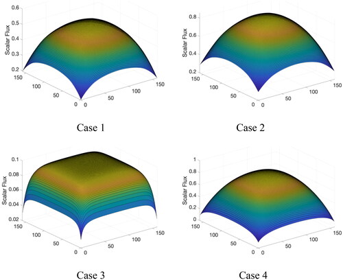
In this section, we demonstrate how the regularity of the exact solution will impact the numerical convergence rate by solving the SN neutron transport equation in its original integro-differential form, using the classic DD and SD methods. The model problem is a 1 cm 1 cm square with the vacuum boundary condition. Thus, there will be no complication from the boundary condition. The S12 level-symmetric quadrature set is used for angular discretization.
We analyze the following four cases: Case 1:
Case 2:
Case 3:
and Case 4:
For all the cases, the external source
Cases 1 and 3 are pure absorption problems, while Case 3 is optically thicker. It is worth noting that the solutions are only determined by the external source for these two cases. Cases 2 and 4 include the scattering effects, while Case 4 is optically thicker and more diffusive. Both the scattering and external source contribute to the solution. The flux distribution calculated with DD for each case is shown in .
Figure 2. Flux distribution on the mesh
The flux errors as a function of mesh size and the rates of convergence are summarized in and for DD and SD, respectively. In and are depicted the error distributions of DD and SD on the mesh
The reference solutions for all the cases are obtained on a very fine mesh (
) using the DD method.
Figure 3. Flux error distribution on the mesh (DD).
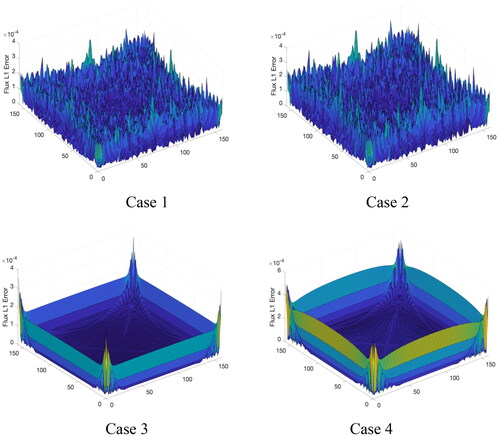
Figure 4. Flux error distribution on the mesh (SD).
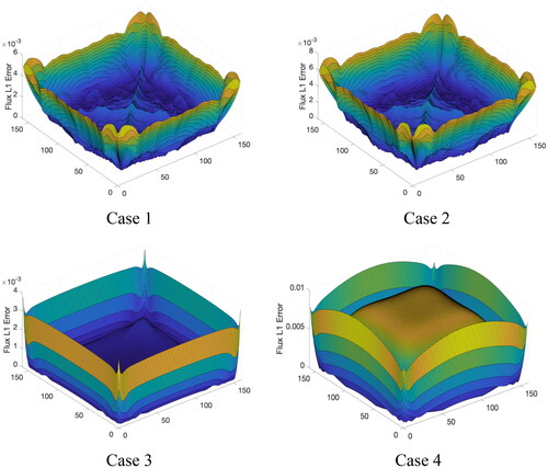
Table 1. Scalar flux errors and convergence rates of DD.
Table 2. Scalar flux errors and convergence rates of SD.
For the DD, it is evident that the convergence rate decreases as the mesh is refined, and the errors are much larger at the boundary. The “noisier” distributions in Cases 1 and 2 are due to the ray effects of the discrete ordinates (SN) method, which are more pronounced in the optically thin problem. The convergence behavior is similar between the cases with and without the scattering, indicating that the source term plays a significant role in defining the irregularity of the solution. Cases 3 and 4 show the improved convergence rate as compared to Cases 1 and 2 because the exponential function in the solution makes the kernel less singular for larger total cross section
In addition, Case 4 has a slightly better rate of convergence than Case 3 on fine meshes (e.g., 1.80 vs. 1.71 on
), because the transport problem in Case 4 becomes more like an elliptic diffusion problem (Wang and Byambaakhuu Citation2021), which usually has better regularity. It is noted that that in Case 3 the convergence rate is only 1.51 on the coarse mesh. It is because for the pure absorption case, the DD becomes unstable when the mesh size is larger than
While for the SD method, the convergence rate is the first order for all the cases. By comparing Cases 4 and 3, the SD method has relatively large error for thick diffusive problems because of the factor
in the error estimate.
Remark 5.1.
The optimal error derived for the DD method is As given by EquationEquation (28)
(28)
(28) , the second derivative
is bounded in the interior of the domain, while it behaves as
near the boundary. Therefore, it is expected that the convergence rate of the DD would decrease with refining the mesh, and asymptotically tend to
It is interesting to note that if the solution were sufficiently smooth (e.g., a manufactured smooth solution), the DD would maintain its second-order accuracy on any mesh size (Wang et al. Citation2019). While for the SD method,
where
or at most
based on the theoretical results given by EquationEquation (28)
(28)
(28) . From the numerical results, we observe that the SD has maintained the first-order convergence on all the meshes.
Remark 5.2.
The scattering does not appear to play a role in defining the smoothness of the solution. For the problem without the external source, if there exists a nonsmooth or anisotropic incoming flux on the boundary, the scattering may not be able to regularize the solution either, since the irregularity caused by the incoming flux, which is defined by the surface integral term of EquationEquation (3)(3)
(3) , has nothing to do with the scattering and the solution flux
6. Conclusions
We have derived the integral kernel for the two-dimensional integral radiation transfer equation, and examined the differential properties of the integral kernel for fulfilling the boundedness conditions of Vainikko’s theorem. We applied the theorem to estimate the derivatives of the radiation transfer solution near the boundary of the domain. It is noted that the first derivative of the scalar flux becomes unbounded when approaching the boundary. The derivatives of order
behave as
for
where
is the distance to the boundary. We have derived the optimal error estimates in terms of the scalar flux for the DD and SD methods. The numerical results demonstrate that the irregularity of the exact transport solution will adversely reduce the rate of convergence of numerical methods. We are currently extending the analysis to the boundary integral transport problem in considering nonzero incoming boundary conditions and corner effects. In addition, it would be interesting to study the convergence behavior of weak numerical solutions.
Disclosure statement
No potential conflict of interest was reported by the authors.
References
- Abramowitz, M., and I. A. Stegun. 1970. Handbook of mathematical functions: With formulas, graphs, and mathematical tables. Dover, New York.
- Agoshkov, V. 1998. Boundary value problems for transport equations. Boston: Birkhauser.
- Altaç, Z. 2007. Exact series expansions, recurrence relations, properties and integrals of the generalized exponential integral functions. J. Quant. Spectrosc. Radiat. Transf 104 (3):310–25. doi:10.1016/j.jqsrt.2006.09.002
- Bell, G. J., and S. Glasstone. 1970. Nuclear reactor theory. New York: Van Nostrand Reinhold Company.
- Case, K. M., and P. F. Zweifel. 1967. Reading, MA: Linear transport theory. Addison-Wesley Publishing Company, Inc.
- de Azevedo, F. S., E. Sauter, P. H. A. Konzen, M. Thompson, and L. B. Barichello. 2018. Integral formulation and numerical simulations for the neutron transport equation in X-Y geometry. Ann. Nucl. Energy 112:735–47. doi:10.1016/j.anucene.2017.10.017
- Egger, H., and M. Schlottbom. 2014. An Lp theory for stationary radiative transfer. Appl. Anal. 93 (6):1283–96. doi:10.1080/00036811.2013.826798
- Germogenova, T. A. 1969. Local properties of the solution of the transport equation. Dokl. Akad. Nauk SSSR 187 (5):978–81.
- Golse, F., P.-L. Lions, B. Perthame, and R. Sentis. 1988. Regularity of the Moments of the Solution of a Transport Equation. J. Funct. Anal. 76 (1):110–25. doi:10.1016/0022-1236(88)90051-1
- Hennebach, E., P. Junghanns, and G. Vainikko. 1995. Weakly singular integral equations with operator-valued Kernels and an application to radiation transfer problems. Integr. Equ. Oper. Theory. 22 (1):37–64. doi:10.1007/BF01195489
- Johnson, C., and J. Pitkaranta. 1983. Convergence of a fully discrete scheme for two-dimensional neutron transport. SIAM J. Math. Anal. 20 (5):951–66.
- Larsen, E. W., and W. F. Miller. Jr., 1980. Convergence rates of spatial difference equations for the discrete-ordinates neutron transport equations in slab geometry. Nucl. Sci. Eng. 73 (1):76–83. doi:10.13182/NSE80-3
- Larsen, E. W. 1982. Spatial Convergence Properties of the Diamond Difference Method in x, y Geometry. Nucl. Sci. Eng. 80 (4):710–713.
- Larsen, E. W., J. E. Morel, and W. F. Miller. Jr., 1987. Asymptotic solutions of numerical transport problems in optically thick, diffusive regimes. J. Comput. Phys. 69 (2):283–324. doi:10.1016/0021-9991(87)90170-7
- Latrach, K. 2001. Compactness results for transport equations and applications. Math. Models Methods Appl. Sci. 11 (07):1181–202. doi:10.1142/S021820250100129X
- Latrach, K., and A. Zeghal. 2012. Existence results for a nonlinear transport equation in bounded geometry on L1-spaces. Appl. Math. Comput. 219 (3):1163–72. doi:10.1016/j.amc.2012.07.026
- Lewis, E. E., and W. F. Miller. Jr., 1993. Computational methods of neutron transport. La Grange Park, Illinois: American Nuclear Society.
- Madsen, N. K. 1972. Convergence of singular difference approximations for the discrete ordinate equations in x−y geometry. Math. Comput. 26 (117):45–50.
- Mikhlin, S. G., and S. Prossdorf. 1986. Singular integral operators. Berlin: Springer-Verlag.
- Mikhlin, S. G. 1965. Multidimensional singular integrals and integral equations. Oxford: Pergamon Press.
- Miller, J., J. H. O’Riordan, and G. I. Shishkin. 2012. Fitted numerical methods for singular perturbation problems. Singapore: World Scientific.
- Pitkäranta, J. 1980. Estimates for the derivatives of solutions to weakly singular fredholm integral equations. SIAM J. Math. Anal. 11 (6):952–68. doi:10.1137/0511085
- Stynes, M., and D. Stynes. 2018. Convection-diffusion problems: An introduction to their analysis and numerical solution. Providence, RI: American Mathematical Society.
- Vainikko, G. 1993. Multidimensional weakly singular integral equations. Berlin Heidelberg: Springer-Verlag.
- Vladimirov, V. S. 1963. Mathematical problems in the one-velocity theory of particle transport. (Translated from, 61, 1961). Chalk River, Ontario: Atomic Energy of Canada Limited.
- Wang, D. 2019. The asymptotic diffusion limit of numerical schemes for the SN transport equation. Nucl. Sci. Eng. 193 (12):1339–54. doi:10.1080/00295639.2019.1638660
- Wang, D. 2022. Error analysis of numerical methods for thick diffusive neutron transport problems on Shishkin Mesh. 2022. Proceedings of International Conference on Physics of Reactors 2022 (PHYSOR 2022), Pittsburgh, PA, USA, May 15-20, 2022, 977986.
- Wang, D., and T. Byambaakhuu. 2021. A new proof of the asymptotic diffusion limit of the SN neutron transport equation. Nucl. Sci. Eng. 195 (12):1347–58. doi:10.1080/00295639.2021.1924048
- Wang, D., T. Byambaakhuu, S. Schunert, and Z. Wu. 2019. Solving the SN transport equation using high order Lax-Friedrichs WENO fast sweeping methods. Proceedings of International Conference on Mathematics and Computational Methods Applied to Nuclear Science and Engineering 2019 (M&C 2019), Portland, OR, USA, August 25–29, 2019, 61–72.
- Wang, Y., and J. C. Ragusa. 2009. On the convergence of DGFEM applied to the discrete ordinates transport equation for structured and unstructured triangular meshes. Nucl. Sci. Eng. 163 (1):56–72. doi:10.13182/NSE08-72