Theory and simulation of objects in liquid crystals

ABSTRACT

Colloidal particles with anisotropic interactions are excellent candidates for synthetic building blocks of self-assembled materials with desirable properties, such as a photonic band-gap or swimming ability, at the nano- or micro-scale. The anisotropic nature of liquid crystals (LCs) makes them an ideal candidate to generate non-spherically symmetric interactions between immersed colloidal particles. Here, we review the progress on the theory and simulation of such systems.

Graphical Abstract

KEYWORDS:

• Liquid crystals
• colloids
• simulations

1. Introduction

The development of designer materials (i.e. materials manufactured to display certain properties rather than randomly tested for the existence of these properties) is an area of active research in both industry and academia. For example, many researchers are attempting to produce photonic crystals (materials with periodicity in their dielectric constant on the nm to µm scale to match the wavelength of light) to replace electronics with faster photonic devices. One promising area of research begins with colloidal suspensions (sub-micron sized particles suspended in a fluid) and uses hydrodynamics to facilitate the self-assembly into crystal structures with periodicity on the scale of nanometers to micrometers. However, in order to design materials with specific properties, one must first be able to model the process used to create them.

A spherical object, such as a colloidal particle, in an anisotropic fluid, like a liquid crystal, behaves very differently from a colloidal particle in a simple fluid. Boundary conditions at the surface of the sphere typically cause the director field (the direction along which the liquid crystal molecules are aligned) to sit parallel or perpendicular to the surface. This makes the colloidal particle in a liquid crystal look like it has poles (parallel alignment) or look like a hedgehog (perpendicular alignment). Such alignments of the liquid crystal field are energetically unfavorable, and to avoid them, topological defects form either on or close to the surface of the sphere [1–3]. This leads to long-range interactions of the colloidal particles mediated by the orientational elasticity of the liquid crystal. Interactions of this sort have been used to self-assemble two-dimensional nematic colloidal crystals which have the potential to be used in a variety of devices. If the liquid crystal is cholesteric, the director field is chiral (it rotates, or has a spatial pitch along one axis). Furthermore, if the colloidal particle has a size comparable to the pitch of the cholesteric, the particle picks up another topological charge related to the twist. Computer modelling can be extremely valuable for studying these systems as they give insights that are often difficult to extract from experiments and allow the modeller to turn on and off certain effects to clearly identify the important properties driving the observed phenomena.

Modelling objects in liquid crystals can present a number of challenges. First, the surface of the object is rarely flat which can be difficult for continuum models where computer simulation techniques typically require discretizations of both the liquid crystal region and the surface, discretizations that may be difficult to match. There is also the difficulty that the objects typically induce topological defects such as disclination lines whose scale (in particular the defect core) are often much smaller than the colloidal object itself. When dynamics are included, all of these issues become more complex as the boundaries are moving, and not in some prescribed manner. The motion of the colloid must be computed from the forces it feels from the liquid crystal media as well as any external forces.

We first review liquid crystal models. Most early work in liquid crystals used Ericksen-Leslie theory which just involves tracking a director field. The problem with such models is that topological defects in the director field are singularities that add significant complexity. Models using a full tensor order parameter gained popularity in the last two decades primarily because such defects arise naturally in such a theory where they involve continuous eigenvalue crossings and no singularities. Adding colloids to these simulations is discussed next and involves hybrid simulations to compute forces on the colloids and track their movement, and corresponding impact on the liquid crystal which simultaneously solving the liquid crystal order parameter and fluid flow equations. We then discuss some of the results obtained using these models.

2. Modelling liquid crystals

The first models to explain liquid crystal phases were mean field theories based on simple free volume arguments by Onsager [4]. While giving a reasonable qualitative description of the aligned phase and transition from the isotropic to nematic states, Onsager’s theory leads to a rather abrupt transition between a strongly ordered nematic and completely disordered isotropic phase. An improved mean field theory, including the introduction of the concept of the ‘molecular field’, was introduced by Maier and Saupe [5,6]. Further improvements by Luckhurst and collaborators [7] provide a fairly quantitative description of the nematic-isotropic transition.

A key aspect of the Maier-Saupe theory is that it leads to a Landau expansion in a tensor order parameter with a cubic term in the order parameter. Such a free energy expansion is the starting point for our description of liquid crystals.

2.1. Bulk free energy of homogeneous system

Following de Gennes [8], the bulk-free energy density of a uniform quiescent thermotropic system is written approximately as

(1) ${\mathcal{F}}_{bulk}(T,\mathbf{Q})=\int d\mathbf{r}a\left[\frac{1}{2}(T-T_0)Q_{ij}^2-\frac{1}{3}B{Q}_{ij}{Q}_{jk}{Q}_{ki}+\frac{1}{4}C{(Q_{ij}^2)}^2\right],$(1)

where $a$, $B$, $C$, and $T_0$ are constants, and $T$ is the temperature. $\mathbf{Q}$ is the order parameter which is a second rank tensor which can be represented by a $3\times 3$ matrix. The eigenvalues of $\mathbf{Q}$ indicate the preference of the system to orient molecules along its three principal axis. The eigenvector associated with the largest eigenvalue is referred to as the director.

The force driving the system back to equilibrium is referred to as the molecular field and is related to the variation derivative of the free energy,

(2) $\mathbf{H}=-\left[\frac{\delta \mathcal{F}}{\delta Q}-\frac{\mathbf{I}}{3}Tr\frac{\delta \mathcal{F}}{\delta Q}\right].$(2)

$\mathbf{H}$ is zero in equilibrium (i.e. the free energy is minimized subject to the constraint that $\mathbf{Q}$ is traceless). The bulk free energy Equation (1)(1) ${\mathcal{F}}_{bulk}(T,\mathbf{Q})=\int d\mathbf{r}a\left[\frac{1}{2}(T-T_0)Q_{ij}^2-\frac{1}{3}B{Q}_{ij}{Q}_{jk}{Q}_{ki}+\frac{1}{4}C{(Q_{ij}^2)}^2\right],$(1) contributes to the molecular field:

(3) ${\mathbf{H}}_{bulk}=-a(T-T_0)\mathbf{Q}+aB\left[{\mathbf{Q}}^2-(\mathbf{I}/3)Tr{\mathbf{Q}}^2\right]-aC\mathbf{Q}Tr{\mathbf{Q}}^2.$(3)

Given that the equilibrium state of $\mathbf{Q}$ is uniaxial and homogeneous, it can be written in the form

$Q_{\alpha \beta }=q({\hat{n}}_{\alpha }{\hat{n}}_{\beta }-{\delta }_{\alpha \beta }/3),$

where $\stackrel{\mathbf{ˆ}}{\mathbf{n}}$ is the director (eigenvector associated with the principal eigenvalue). The amplitude $q$ of the order parameter is given by the condition that the molecular field is zero yielding

(4) $q=\frac{B}{4C}\left(1+\sqrt{1-\frac{24C}{B^2}(T-T_0)}\right).$(4)

There is a first-order phase transition where $q$ changes discontinuously to zero at the transition temperature $T_c$ between the nematic (N) and isotropic (I) phase (often referred to as the clearing point) which is

(5) $T_c=T_0+\frac{B^2}{27C}.$(5)

To match to experimental data, it is useful to use Equation (5)(5) $T_c=T_0+\frac{B^2}{27C}.$(5) to eliminate $T_0$ from Equation (4)(4) $q=\frac{B}{4C}\left(1+\sqrt{1-\frac{24C}{B^2}(T-T_0)}\right).$(4) and then use the experimental value of $T_c$. A subsequent fit to a measurement of $q(T)$ then yields the parameters $B$ and $C$.

One difficulty that arises is that an examination of the literature shows variations of the order of 20% in different measurements of $q(T)$ in the same material [9–19]. In most cases, this is substantially more than the statistical error inherent in the individual experiments. It would appear that the main source of discrepancy can be found in different sources of normalization. Most experiments, especially those based on measuring refractive indices, yield data only on the relative value of the order parameter and do not give absolute measurements. A few different techniques have been used for normalization. One method just normalizes the data to some previous measurement. For instance, Karat and Madhusudana [10] normalize their data (from measurements of refractive indices) for the material 7CB to a measurement of the order parameter at a single temperature done with Raman scattering several years earlier by other researchers. Unfortunately, this measurement is not in agreement with the latter Raman scattering by Dalmolen and collaborators [11], nor is it consistent with NMR measurements of 5CB by Emsley [13]. However, if one takes Karat and Madhusudana’s raw data and normalize it by either the Raman data of Dalmolen or the NMR data of Emsley one finds good agreement between all three data sets. Another normalization method extrapolates the data back to absolute zero temperature and then assumes that the order parameter should be unity there. The justification for this is usually based on the observation that often the data appears to follow a power law [9],

(6) $q(T)=A{\left(1-\frac{T}{T_c+\mathrm{\Delta }}\right)}^b,$(6)

where $A$, $b$, and $\mathrm{\Delta }$ are constants. This is what one might expect for a second-order phase transition (at $T_c+\mathrm{\Delta }$) preempted by a first-order transition (at $T_c$). Such a relationship is a straight line on a log-log plot (of $q$ versus $1-T/(T_c+\mathrm{\Delta })$) and can thus be extrapolated fairly easily to zero temperature. When the nematic phase covers several decades in temperature this seems to give reasonably consistent results. However, for many pure compounds, the nematic phase covers only 10–15 ${ }^{\circ }C$ so that the extrapolation can be a major systematic source of uncertainty. In fitting experimental data, we have normalized data based on measurements of refractive indices by either data based on NMR or Raman scattering if available in preference to extrapolation. The results are shown in Figure 1. The parameters for the fits are given in Table 1. Two different fits were performed. One is a straightforward fit to Equation (4)(4) $q=\frac{B}{4C}\left(1+\sqrt{1-\frac{24C}{B^2}(T-T_0)}\right).$(4) , making use of the known transition temperatures to eliminate $T_0$. The free energy Landau-de Gennes expansion does not do a good job of fitting the experimental data very close to the transition. As a result, data within ${2.5}^{\circ }$C of the transition were excluded in order to improve the fit in the rest of the nematic temperature range. This is shown as a dashed line in Figure 1.

Table 1. Transition temperatures (experimental, $T_c$ is nematic-isotropic transition and $T_{CN}$ is the crystal-nematic transition except for 8CB where it is the smectic A-nematic transition) and coefficients of mean field free energy and power-law scaling from fitting to experimental data (see text). In cases where multiple data sets are used, all data were given equal weight. Experimental data from Ref [9–14] for 5CB, 6CB, 7CB and 8CB. Experimental data for 5OCB, 6OCB, 7OCB, 8OCB from Ref [9,15,16]. PAA data from [9,17,18]. MBBA data from [19]. Results for 5CB, PAA, and MBBA are shown in Figure 1.

material	$T_{CN}{(}^{\circ }C)$	$T_c{(}^{\circ }C)$	$T_0{(}^{\circ }C)$	$B(K)$	$C(K)$	$A$	$\mathrm{\Delta }{(}^{\circ }C)$	$b$
5 CB	22.5	35.0	17.0	372	285	0.712	0.268	0.161
6 CB	13.8	28.8	15.3	284	222	0.719	0.227	0.171
7 CB	28.5	42.0	21.4	369	244	0.835	0.353	0.163
8 CB	33.3	40.1	31.7	181	143	0.803	0.556	0.174
5 OCB	47.5	68.0	52.1	349	284	0.841	0.116	0.208
6 OCB	57.0	75.5	67.0	188	154	0.973	0.168	0.211
7 OCB	53.5	75.0	62.1	274	218	0.913	0.012	0.205
8 OCB	67.0	80.0	68.7	263	227	0.810	0.065	0.175
MBBA	22.0	48.0	30.5	410	355	0.717	1.28	0.216
PAA	119.5	136.5	123	337	315	0.857	1.60	0.212

Fits to Equation (6)(6) $q(T)=A{\left(1-\frac{T}{T_c+\mathrm{\Delta }}\right)}^b,$(6) are shown as the solid line in Figure 1. As can be seen, this fit gives a better match to the data in the vicinity of the transition. It would be of interest to examine whether adding fluctuations to the mean field models described here would yield better agreement in the vicinity of the transition. There is some suggestion from renormalization group calculations and Monte Carlo simulations that this might be the case [8].

Figure 1. Magnitude of order parameter $q$ versus temperature measured relative to clearing point temperature (in Kelvin). Left: 5CB. Symbol shapes correspond to experimental data from Ref [9]. (diamonds) [10], (stars) [11], (squares) [12], (triangles), and [13]. Middle: PAA. Data from [9] (diamonds) and [17,18] (stars). Right: MBBA. Data from [19]. Dashed lines are fits to Equation (4)(4) $q=\frac{B}{4C}\left(1+\sqrt{1-\frac{24C}{B^2}(T-T_0)}\right).$(4) and solid lines are fits to Equation (6).

Note that it is impossible to obtain the overall scale factor $a$ from a homogeneous equilibrium measurement. In most cases, this factor can be incorporated into an overall diffusion constant. The one place where it does play a role is in the size of a defect core. In a typical ${\varphi }^4$ theory, the width of an interface is proportional to $\sqrt{\kappa /aC}$ where $\kappa$ is the coefficient of a square gradient term. One might expect the size of a defect core to follow a similar relationship.

In some cases, the only data one can obtain is the transition temperatures. In this case, one can still make a reasonable estimate based either on data from similar materials or from a simple theory such as the Maier-Saupe model [5,6,8]. In the Maier-Saupe model, $q=0.43$ at the transition temperature and $q=1$ at absolute zero. If you fit these values using the observed transition temperature, you are probably within about 10% of the correct values over most of the temperature range for most materials.

The bulk free energy sets the equilibrium order parameter $q$ and in most simulations, this is all that is needed, i.e. the order parameter in the system does not deviate from the equilibrium value in any substantial way, except in the core of topological defects. In other cases, particularly in shear with models where the magnitude of the order parameter is directly enhanced by the shear flow field, the value of $q$ in the simulation can change significantly from the equilibrium value. In the most extreme cases, the value of $q$ in the simulation may fall outside of a physically reasonable range (As $\mathbf{Q}$ is related to the second moment of a probability distribution, and $n$ is a unit vector, the eigenvalues $\lambda$ of $\mathbf{Q}$, of which $q$ is the largest, should satisfy $-1/3<\lambda <2/3$). One option to ‘fix’ this problem is to change the fourth-order term in the bulk free energy to a logarithmic term with a divergence as you approach the edge of the physical values for the eigenvalues. Proposals have included terms such as [20]

(7) $-c_m^{4}ln\left(1-|Q{|}^4/c_m^4\right)$(7)

which induce a divergence when $|Q|$ approaches $c_m$. Alternatively, one could use the spectral radius of $\mathbf{Q}$ to ensure physical values of the order parameter. While such functionals are helpful to explore the full range of the model, there is at present no actual data from experiments or molecular dynamics that tell us that this is the correct form for the free energy. It is also possible that the system could transition to another phase (e.g. smectic) or start to become disordered due to generation of topological defects [21] in some cases. In the simulations with colloids described in this review, the normal Landau-de Gennes model is sufficient to yield physically realistic results.

2.2. Elastic free energy

Distortion of the order parameter field generally costs free energy. Microscopically this is related to the correlation of molecular orientation across a finite distance. One can also create a square gradient style theory from purely phenomenological grounds. The phenomenological theory based on gradients of the director has been very successful. This theory is fairly old and the resulting free energy density is generally referred to as the Frank free energy [8,22]:

(8) ${\mathcal{F}}_d=\int d\mathbf{r}\left[\frac{1}{2}{K}_1{(\mathrm{\nabla }\cdot \mathbf{n})}^2+\frac{1}{2}{K}_2{(\mathbf{n}\cdot \mathrm{\nabla }\times \mathbf{n})}^2+\frac{1}{2}{K}_3{(\mathbf{n}\times \mathrm{\nabla }\times \mathbf{n})}^2\right].$(8)

where $K_1$, $K_2$, and $K_3$ are the splay, twist, and bend elastic constants, respectively, and $\mathbf{n}$ is the director.

Early attempts to obtain a similar theory based on the tensor order parameter suffered from having only two elastic constants $L_1$ and $L_2$. These two constants corresponded to the two lowest order terms in a gradient expansion. The problem that arises in getting another elastic constant is that at the next highest order in the gradient expansion there are another six possible constants (for a total of eight). This makes for a somewhat impracticable situation. Fortunately, it has been found to be adequate to include only one of these extra terms (adding some terms gives an unrealistic dependence of the elastic constants on $q$) [23–25]. This gives a distortion energy

(9) ${\mathcal{F}}_d=\int d\mathbf{r}\left[\frac{L_1}{2}({\mathrm{\partial }}_{\alpha }{Q}_{\beta \gamma })({\mathrm{\partial }}_{\alpha }{Q}_{\beta \gamma })+\frac{L_2}{2}({\mathrm{\partial }}_{\alpha }{Q}_{\alpha \gamma })({\mathrm{\partial }}_{\beta }{Q}_{\beta \gamma })+\frac{L_3}{2}{Q}_{\alpha \beta }({\mathrm{\partial }}_{\alpha }{Q}_{\gamma \epsilon })({\mathrm{\partial }}_{\beta }{Q}_{\gamma \epsilon })\right].$(9)

The elastic contribution to the molecular field then becomes

(10) $\begin{array}{rl}& ({\mathbf{H}}_d{)}_{\alpha \beta }=L_1({\mathrm{\partial }}_{\gamma }^2{Q}_{\alpha \beta })+L_2\left[\frac{1}{2}({\mathrm{\partial }}_{\alpha }{\mathrm{\partial }}_{\gamma }{Q}_{\gamma \beta }+{\mathrm{\partial }}_{\beta }{\mathrm{\partial }}_{\gamma }{Q}_{\gamma \alpha })-\frac{1}{3}{\delta }_{\alpha \beta }{\mathrm{\partial }}_{\gamma }{\mathrm{\partial }}_{\epsilon }{Q}_{\gamma \epsilon }\right]+\\ & \frac{1}{2}{L}_3\left[{\mathrm{\partial }}_{\gamma }(Q_{\gamma \epsilon }{\mathrm{\partial }}_{\epsilon }{Q}_{\alpha \beta })-({\mathrm{\partial }}_{\alpha }{Q}_{\gamma \epsilon })({\mathrm{\partial }}_{\beta }{Q}_{\gamma \epsilon })+\frac{1}{3}{\delta }_{\alpha \beta }{({\mathrm{\partial }}_{\eta }{Q}_{\gamma \epsilon })}^2\right].\end{array}$(10)

If we assume uniaxial symmetry and put $Q_{\alpha \beta }=q(n_{\alpha }{n}_{\beta }-\frac{1}{3}{\delta }_{\alpha \beta })$ into this expression this can be mapped onto the Frank free energy. To obtain the equivalent mapping one must take [23–25]

(11) $\begin{array}{rl}& L_1=(3K_2-K_1+K_3)/(6q^2),\\ & L_2=(K_1-K_2)/q^2,\\ & L_3=(K_3-K_1)/(2q^3).\end{array}$(11)

The reverse mapping is somewhat instructive and gives

(12) $\begin{array}{rl}& K_1=(2L_1+L_2)q^2-\frac{2}{3}{L}_3{q}^3,\\ & K_2=2L_1{q}^2-L_3{q}^3,\\ & K_3=(2L_1+L_2)q^2+\frac{4}{3}{L}_3{q}^3.\end{array}$(12)

Note that if you take $L_2=L_3=0$ you arrive at the common ‘one-elastic’ constant theory (in the director picture) where $K_1=K_2=K_3$. If you take $L_3=0$ then $K_1=K_3$ but distinct from $K_2$. Figure 2 shows the elastic constants for 5CB. As is typical, the constants are actually quite different, with the smallest being the twist, followed by the splay, and then the bend. What this means is that if a distortion can be accommodated by either splay or bend, it will typically be accommodated by splay as this will cost less.

Figure 2. Elastic constants versus temperature for 5CB. Data points from [26] are shown in symbols and the curves are from Equation (12)(12) $\begin{array}{rl}& K_1=(2L_1+L_2)q^2-\frac{2}{3}{L}_3{q}^3,\\ & K_2=2L_1{q}^2-L_3{q}^3,\\ & K_3=(2L_1+L_2)q^2+\frac{4}{3}{L}_3{q}^3.\end{array}$(12) using the values for $L_i$ shown in Table 2 and using the values of $q$ from the power law fit with parameters in Table 1.

Table 2. Constants for some common liquid crystals. Elastic constants are in pN. Data used for the fit for 5CB elastic constants come from [26]. Data for 5CB dielectric constants are from [28]. Values for PAA are from [24]. Note that these values should only be used over the temperature range where these materials are in the nematic phase.

material	$L_1$ (pN)	$L_2$ (pN)	$L_3$ (pN)	${\epsilon }_m$	${\epsilon }_a$
5 CB	7.4	6.4	8.2	11.0	33.4
PAA	10.5	13.9	20

Experimental data primarily exist for measurements of the $K_i$ values, from which one can deduce the $L_i$ using Equation (11)(11) $\begin{array}{rl}& L_1=(3K_2-K_1+K_3)/(6q^2),\\ & L_2=(K_1-K_2)/q^2,\\ & L_3=(K_3-K_1)/(2q^3).\end{array}$(11) . Using data from [26] and the values of $q$ from the power-law fits given in Table 1, one finds that the variation in $L_i$ as a function of temperature is negligible compared to that for the $K_i$, i.e. the variation in temperature is captured by the changes in $q$. This can be seen in Figure 2. The other thing to note is that while $L_2=L_3=0$ is often employed as equivalent to the ‘one-elastic constant approximation’, the actual values for the $L_i$, given in Table 2 are actually quite similar, unlike the values of $K_i$ which differ by a much larger factor for 5CB. A similar fit from [24] provides data for PAA.

If, in addition, one wants to model a cholesteric, an additional term is added to the free energy density:

(13) $f_c=\frac{4\pi L_1}{P}{\epsilon }_{\alpha \beta \gamma }{Q}_{\alpha \nu }({\mathrm{\partial }}_{\beta }{Q}_{\gamma \nu }),$(13)

where ${\epsilon }_{\alpha \beta \gamma }$ is the Levi-Civita tensor. This results in a free energy minima when the helical pitch in the cholesteric is equal to $P$. While it is common to use a one elastic constant approximation when modeling liquid crystals, real cholesterics typically have a small $K_2$ compared to $K_1$ and $K_2$. If you do not match this in a simulation and use a one-elastic constant approximation, typically one will induce a blue-phase rather than a cholesteric [27].

2.3. Dielectric response

The optical response of the liquid crystal is embodied in the (relative) dielectric tensor [8]:

(14) ${\epsilon }_{\alpha \beta }=\frac{2}{3}{\epsilon }_a{Q}_{\alpha \beta }+{\epsilon }_m{\delta }_{\alpha \beta }.$(14)

In a nematic, this can be related to the order parameter $q$ via

(15) ${\epsilon }_a=\frac{3}{2q}({\epsilon }_{||}-{\epsilon }_{\mathrm{\perp }}),{\epsilon }_m\frac{2}{3}{\epsilon }_{\mathrm{\perp }}+\frac{1}{3}{\epsilon }_{||}$(15)

and ${\epsilon }_{||}$ and ${\epsilon }_{\mathrm{\perp }}$ are the relative permittivity along and perpendicular to the nematic director. Fitting the data in [28] for ${\epsilon }_{||}$ and ${\epsilon }_{\mathrm{\perp }}$, of $q$ from the power-law fits given in Table 1, one finds that the variation in ${\epsilon }_a$ and ${\epsilon }_m$ as a function of temperature is negligible, i.e. as with the elastic constants, the entire temperature dependence comes from that in the order parameter $q$. The values for ${\epsilon }_a$ and ${\epsilon }_m$ for 5CB are given in Table 2. The high ratio of ${\epsilon }_{||}/{\epsilon }_{\mathrm{\perp }}$ is what makes a liquid crystal such a useful material for optical devices (as the relative permeability determines the index of refraction). It also makes it difficult to predict the optical response (or deduce the configuration of the director from the optical response) in situations where the director is not uniform. However, the full optical response, including the photonic band structure, can be computed directly from a knowledge of $Q_{\alpha \beta }$, something that is readily available from a simulation [29,30].

It is fairly easy to affect the director orientation with a strong electric field (this is the basis of liquid crystal displays) so that using optical tweezers to move colloids in a liquid crystal will inevitably affect the local orientation. This effect can be captured by the contribution of the electric field to the free energy,

(16) ${\mathcal{F}}_E=\frac{1}{4\pi }\int D\cdot dE=-\frac{{\epsilon }_m}{8\pi }{E}^2-\frac{{\epsilon }_a}{12\pi }{E}_{\alpha }{E}_{\beta }{Q}_{\alpha \beta }.$(16)

This leads to a contribution to the molecular field of

(17) $(H_E{)}_{\alpha \beta }=\frac{{\epsilon }_a}{12\pi }\left(E_{\alpha }{E}_{\beta }-\frac{{\delta }_{\alpha \beta }}{3}{E_{\gamma }}^2\right).$(17)

2.4. Dynamics

Theories for the dynamics of liquid crystals are primarily based on linear response theory [31]. The starting point for such theories is the entropy source from the dissipation $T\dot{S}$. It is then customary to write each contribution to the entropy source as the product of a ‘flux’ by the conjugate ‘force’. This methodology has been followed by a number of authors [23,32,33] with general agreement for the entropy source to be

(18) $T\dot{S}=\frac{d{Q}_{\alpha \beta }}{dt}{H}_{\alpha \beta }+{\sigma }_{{ }_{\alpha \beta }}^{\prime }{\mathrm{\partial }}_{\beta }{u}_{\alpha }$(18)

where ${\sigma }_{{ }_{\alpha \beta }}^{\prime }$ is the viscous stress. The total stress appears in the Navier-Stokes equation for the fluid flow,

(19) $\rho ({\mathrm{\partial }}_t+u_{\beta }{\mathrm{\partial }}_{\beta })u_{\alpha }={\mathrm{\partial }}_{\beta }{\sigma }_{\alpha \beta }.$(19)

We divide the total stress into viscous stress ${\sigma }_{{ }_{\alpha \beta }}^{\prime }$ and the ‘equilibrium stress’ ${\sigma }_{\alpha \beta }^e$:

(20) ${\sigma }_{\alpha \beta }={\sigma }_{{ }_{\alpha \beta }}^{\prime }+{\sigma }_{\alpha \beta }^e.$(20)

The reversible, or equilibrium, stress is obtained from the variation of the free energies described in the previous sections. It can be obtained in an entirely analogous manner to the way the Eriksen stress is derived in Chapter three of de Gennes book [8] for the director description. It is found to be

(21) ${\sigma }_{\alpha \beta }^e=-{\mathrm{\partial }}_{\beta }{Q}_{\gamma \nu }\frac{\delta \mathcal{F}}{\delta {\mathrm{\partial }}_{\alpha }{Q}_{\gamma \nu }}-p{\delta }_{\alpha \beta },$(21)

Incompressibility requires that the isotropic pressure $p$ satisfy

(22) $p=p_0-F_d$(22)

where $p_0$ is the ambient pressure (i.e. usually 1 atmosphere) and $F_d$ is the free energy density. In simulations, it is usually convenient to take $p_0=\rho a_0$ ($a_0$ is the isentropic compressibility); however, if one was to examine fully compressible flows with a varying density field a more realistic form would probably be required. In the lattice-Boltzmann formulation, one usually selects $a_0=1/3\mathrm{\Delta }{x}^2/\mathrm{\Delta }{t}^2$ and ensures that $\mathrm{\Delta }x$ and $\mathrm{\Delta }t$ are chosen so that all fluid velocities in the simulation are much smaller than $\sqrt{a_0}$. In this case, the density in the simulation is very nearly constant and the parameter $a_0$ has little impact on the results.

It is important that the Navier-Stokes equation be written here in component form. This is due to the presence of two opposite conventions in the literature for the definition of the stress tensor. In one convention, the divergence of the stress tensor acts on the first index (i.e. on $\alpha$ rather than the second $\beta$ which we use here) so that the left-hand side is the material derivative of the $\beta$ component of the velocity. As a result, the stress tensor is the transpose of what we would obtain with our convention. Normally, with a symmetric stress tensor, this is unimportant. However, here we have an antisymmetric part to the stress tensor and so must be careful that we do not obtain the wrong sign. If you use the vector notation, rather than give the component form, there is no way of knowing which convention is being used (i.e. whether to take the divergence to act on the first or second index of the stress tensor).

It is useful to separate out the anti-symmetric part of viscous stress tensor. The anti-symmetric part is

(23) ${\tau }_{\alpha \beta }=Q_{\alpha \gamma }{H}_{\gamma \beta }-H_{\alpha \gamma }{Q}_{\gamma \beta }.$(23)

Most models in the literature which are complete enough to include an anti-symmetric part agree on the form (or something equivalent after doing some algebra) of this term. There are some discrepancies on the sign, however, which appear to be related to the different conventions used for the stress tensor. The sign used here is consistent with the torque in the Ericksen-Leslie formalism for the director field.

With these definitions, the entropy source may be written as

(24) $\begin{array}{rl}& T\dot{S}=\frac{d{Q}_{\alpha \beta }}{dt}{H}_{\alpha \beta }+{\sigma }_{\alpha \beta }^s{D}_{\alpha \beta }+{\tau }_{\alpha \beta }{\mathrm{\Omega }}_{\alpha \beta },\\ & =\frac{\delta Q_{\alpha \beta }}{\delta t}{H}_{\alpha \beta }+{\sigma }_{\alpha \beta }^s{D}_{\alpha \beta }.\end{array}$(24)

where ${\sigma }_{\alpha \beta }^s$ is the symmetric part of the viscous stress, $\mathbf{D}=(\mathbf{W}+{\mathbf{W}}^T)/2$ is the symmetric part of $\mathbf{W}={\mathrm{\partial }}_{\beta }{u}_{\alpha }$ and $\mathrm{\Omega }=(\mathbf{W}-{\mathbf{W}}^T)/2$ is the anti-symmetric part. The rate of change of the order parameter is now given by a corotational derivative

(25) $\frac{\delta Q_{\alpha \beta }}{\delta t}=({\mathrm{\partial }}_t+u_{\gamma }{\mathrm{\partial }}_{\gamma })Q_{\alpha \beta }+Q_{\alpha \gamma }{\mathrm{\Omega }}_{\gamma \beta }-{\mathrm{\Omega }}_{\alpha \gamma }{Q}_{\gamma \beta },$(25)

where $\mathrm{\Omega }=(\mathbf{W}-{\mathbf{W}}^T)/2$ is the anti-symmetric part of $\mathbf{W}={\mathrm{\partial }}_{\beta }{u}_{\alpha }$. The corotational derivative gives the rate of change of the order parameter with respect to the background fluid.

As is standard when dealing with irreversible processes, one defines fluxes and forces by writing each contribution to the entropy source as the product of a ‘flux’ and a conjugate ‘force’. However, while each flux and force is paired in the entropy production, which one is called the flux versus force is a matter of convention. Different choices lead to different, but equivalent, linear response theories. We follow the convention in [23] which leads to

(26) ${\sigma }_{\alpha \beta }^s=R_{\alpha \beta \gamma \mu }{D}_{\gamma \mu }-M_{\alpha \beta \gamma \mu }{H}_{\gamma \mu },$(26)

(27) $\frac{\delta Q_{\alpha \beta }}{\delta t}={M_{\alpha \beta \gamma \mu }}^{\prime }{D}_{\gamma \mu }+P_{\alpha \beta \gamma \mu }{H}_{\gamma \mu },$(27)

where the coefficients $R$, $M$, $M^{\prime }$, and $P^{\prime }$ may be functions of the fields $\rho$ and $\mathbf{Q}$. In addition, one should ensure that constraints, such as the traceless nature or $\mathbf{Q}$ and incompressibility are typically imposed via the method of Lagrange multipliers [8,33] or its equivalent. It is in the choice of these coefficients that the different models in the literature vary widely. Onsager reciprocity requires that

(28) $M_{\alpha \beta \gamma \mu }={M_{\alpha \beta \gamma \mu }}^{\prime }.$(28)

In the model of Beris and Edwards [23], the coefficients are most typically chosen as

(29) $\begin{array}{rl}& R_{\alpha \beta \gamma \mu }=\frac{\eta }{2}({\delta }_{\alpha \gamma }{\delta }_{\beta \mu }+{\delta }_{\alpha \mu }{\delta }_{\beta \gamma })\\ & +\frac{{\beta }_2}{2}(Q_{\alpha \gamma }{\delta }_{\beta \mu }+Q_{\alpha \mu }{\delta }_{\beta \gamma }+{\delta }_{\alpha \mu }{Q}_{\beta \gamma }+{\delta }_{\alpha \gamma }{Q}_{\beta \mu })\\ & M_{\alpha \beta \gamma \mu }=\frac{2\xi }{3}({\delta }_{\alpha \gamma }{\delta }_{\beta \mu }+{\delta }_{\alpha \mu }{\delta }_{\beta \gamma })+\frac{\xi }{2}(Q_{\alpha \gamma }{\delta }_{\beta \mu }+Q_{\alpha \mu }{\delta }_{\beta \gamma }+{\delta }_{\alpha \mu }{Q}_{\beta \gamma }+{\delta }_{\alpha \gamma }{Q}_{\beta \mu })\\ & -2\xi (Q_{\alpha \beta }+\frac{1}{3}{\delta }_{\alpha \beta })Q_{\gamma \mu }\\ & P_{\alpha \beta \gamma \mu }=\frac{\mathrm{\Gamma }}{2}({\delta }_{\alpha \gamma }{\delta }_{\beta \mu }+{\delta }_{\alpha \mu }{\delta }_{\beta \gamma }),\end{array}$(29)

where $\eta$ and ${\beta }_2$ are viscosity coefficients (constants), and $\mathrm{\Gamma }$ is a rotational diffusion constant for $\mathbf{Q}$. $\xi$ is a constant between 0 and 1 and is related to the aspect ratio of the molecules. Higher order (in $\mathbf{Q}$) terms are possible but not typically used as there are already sufficient parameters to match to experimental data. The higher order term in $M$ is related to the Lagrange multiplier necessary to keep $\mathbf{Q}$ and ${\sigma }^s$ traceless.

Putting this all together leads to the equation of motion for $\mathbf{Q}$

(30) $\frac{\delta Q_{\alpha \beta }}{\delta t}=\xi D_{\alpha \gamma }(Q_{\gamma \beta }+\frac{1}{3}{\delta }_{\gamma \beta })+\xi (Q_{\alpha \gamma }+\frac{1}{3}{\delta }_{\alpha \gamma })D_{\gamma \beta }-2\xi (Q_{\alpha \beta }+\frac{1}{3}{\delta }_{\alpha \beta })Q_{\gamma \mu }{D}_{\gamma \mu }+\mathrm{\Gamma }{H}_{\alpha \beta },$(30)

where the left-hand side is the corotational derivative given in Equation (25)(25) $\frac{\delta Q_{\alpha \beta }}{\delta t}=({\mathrm{\partial }}_t+u_{\gamma }{\mathrm{\partial }}_{\gamma })Q_{\alpha \beta }+Q_{\alpha \gamma }{\mathrm{\Omega }}_{\gamma \beta }-{\mathrm{\Omega }}_{\alpha \gamma }{Q}_{\gamma \beta },$(25) . In addition, we have the Navier-Stokes equation

(31) $\rho ({\mathrm{\partial }}_t+u_{\beta }{\mathrm{\partial }}_{\beta })u_{\alpha }={\mathrm{\partial }}_{\beta }{\sigma }_{\alpha \beta }^s+{\mathrm{\partial }}_{\beta }{\sigma }_{\alpha \beta }^e+{\mathrm{\partial }}_{\beta }{\tau }_{\alpha \beta },$(31)

where $\tau$ is given by Equation (23)(23) ${\tau }_{\alpha \beta }=Q_{\alpha \gamma }{H}_{\gamma \beta }-H_{\alpha \gamma }{Q}_{\gamma \beta }.$(23) , ${\sigma }^e$ is given by Equation (21)(21) ${\sigma }_{\alpha \beta }^e=-{\mathrm{\partial }}_{\beta }{Q}_{\gamma \nu }\frac{\delta \mathcal{F}}{\delta {\mathrm{\partial }}_{\alpha }{Q}_{\gamma \nu }}-p{\delta }_{\alpha \beta },$(21) , and ${\sigma }^s$ is

${\sigma }_{\alpha \beta }^s=R_{\alpha \beta \gamma \mu }{D}_{\gamma \mu }-\xi D_{\alpha \gamma }(Q_{\gamma \beta }+{\delta }_{\gamma \beta }/3)-\xi (Q_{\alpha \gamma }+{\delta }_{\alpha \gamma }/3)D_{\gamma \beta }$

(32) $+2\xi (Q_{\alpha \beta }+{\delta }_{\alpha \beta }/3)Q_{\gamma \mu }{D}_{\gamma \mu }.$(32)

There has been some attempts to derive equations from a molecular kinetic theory picture, primarily by Doi and collaborators [34–37]. The resulting equation for the evolution of $\mathbf{Q}$ is very similar to Equation (30)(30) $\frac{\delta Q_{\alpha \beta }}{\delta t}=\xi D_{\alpha \gamma }(Q_{\gamma \beta }+\frac{1}{3}{\delta }_{\gamma \beta })+\xi (Q_{\alpha \gamma }+\frac{1}{3}{\delta }_{\alpha \gamma })D_{\gamma \beta }-2\xi (Q_{\alpha \beta }+\frac{1}{3}{\delta }_{\alpha \beta })Q_{\gamma \mu }{D}_{\gamma \mu }+\mathrm{\Gamma }{H}_{\alpha \beta },$(30) , except with $\xi =1$ due to the assumption of infinite aspect ratio (i.e. very long thin rods). This imposes only affine deformations of $\mathbf{Q}$ by the flow field [23] and results in only steady states in shear. The lack of any ‘tumbling’ states in high shear was originally put down the choice of the fourth moment in the model. However, it seems more likely that the lack of tumbling is related to the imposed affine deformations as $\xi <1$ does have a tumbling regime [20,38]. The stress for the Doi model typically does not include the terms in $M$ at order $\mathbf{Q}$ or higher (while these terms are included in $M^{\prime }$) so the result is that Onsager reciprocity is only followed to first order in $\mathbf{Q}$ in such theories.

2.5. Ericksen-Leslie equations

The Ericksen-Leslie (ELP) equations describe the dynamics of uniaxial nematic liquid crystals in terms of a single director $\mathbf{n}$. As such they should be a limit of the dynamics described above. One might question why we are not trying to obtain these equations, rather than the ones for the tensor order parameter. This is answered by de Gennes [8]: ‘The description does not include disclination lines (or points). In practice, the lines may play a significant role in certain dissipative flow properties. This implies that all hydrodynamics experiments devised to check the ELP equations are meaningful only if all disclinations are carefully eliminated from the sample, and from all upstream regions.’ However, since the ELP theory was the only useable theory for a large number of years, most experimental data are reported in terms of coefficients in these equations. As a result, it is useful to match the descriptions.

The Ericksen-Leslie equations are [8]

(33) ${\sigma }_{\alpha \beta }={\alpha }_1{n}_{\alpha }{n}_{\beta }{n}_{\mu }{n}_{\rho }{D}_{\mu \rho }+{\alpha }_4{D}_{\alpha \beta }+{\alpha }_5{n}_{\beta }{n}_{\mu }{D}_{\mu \alpha }$(33)

(34) $+{\alpha }_6{n}_{\alpha }{n}_{\mu }{D}_{\mu \beta }+{\alpha }_2{n}_{\beta }{N}_{\alpha }+{\alpha }_3{n}_{\alpha }{N}_{\beta },$(34)

(35) $h_{\mu }={\gamma }_1{N}_{\mu }+{\gamma }_2{n}_{\alpha }{D}_{\alpha \mu }$(35)

together with the relations

(36) ${\gamma }_1={\alpha }_3-{\alpha }_2,$(36)

(37) ${\gamma }_2={\alpha }_6-{\alpha }_5={\alpha }_2+{\alpha }_3.$(37)

The last of these relations is known as Parodi’s relation and is a result of Onsager reciprocity. Here we have written the stress tensor using the convention above (it is the transpose of the one used in de Gennes) so that in the corresponding Navier-Stokes equation one contracts on the second index of the stress tensor in the divergence. The distortion stress and pressure are grouped separately and are referred to as the Ericksen stress. The $N_{\alpha }$ are co-rotational derivatives,

(38) $N_{\alpha }={\mathrm{\partial }}_t{n}_{\alpha }+u_{\beta }{\mathrm{\partial }}_{\beta }{n}_{\alpha }-(\omega \times \mathbf{n}{)}_{\alpha }$(38)

(39) $={\mathrm{\partial }}_t{n}_{\alpha }+u_{\beta }{\mathrm{\partial }}_{\beta }{n}_{\alpha }+{\mathrm{\Omega }}_{\alpha \mu }{n}_{\mu }$(39)

where $\omega =\mathrm{\nabla }\times \mathbf{u}/2$. The molecular field $\mathbf{h}$ is

(40) $h_{\mu }=-\frac{\delta \mathcal{F}}{\delta n_{\mu }}$(40)

(41) $=K_{EL}{\mathrm{\nabla }}^2{n}_{\mu }+\zeta (\mathbf{r})n_{\mu }$(41)

where the last line is true under the one-elastic constant approximation and $\zeta$ is a Lagrange multiplier to fix ${\mathbf{n}}^2=1$ (one can always add to $\mathcal{F}$ a term of the form $\zeta (\mathbf{r}){\mathbf{n}}^2/2=\zeta (\mathbf{r})/2$ without changing the distortion energy).

To obtain the ELP equations from the tensor formalism we impose uniaxial symmetry on the order parameter, similar to what was done in Section 2.2 for the elastic contribution to the free energy. The resulting mapping gives the Leslie coefficients as [32,39]

(42) ${\alpha }_1=-\frac{2}{3}{q}^2(3+4q-4q^2){\xi }^2\frac{1}{\mathrm{\Gamma }},$(42)

(43) ${\alpha }_2=(-\frac{1}{3}q(2+q)\xi -q^2)\frac{1}{\mathrm{\Gamma }},$(43)

(44) ${\alpha }_3=(-\frac{1}{3}q(2+q)\xi +q^2)\frac{1}{\mathrm{\Gamma }},$(44)

(45) ${\alpha }_4=\frac{4}{9}(1-q{)}^2{\xi }^2\frac{1}{\mathrm{\Gamma }}+\eta -\frac{2}{3}q{\beta }_2,$(45)

(46) ${\alpha }_5=(\frac{1}{3}q(4-q){\xi }^2+\frac{1}{3}q(2+q)\xi )\frac{1}{\mathrm{\Gamma }}+q{\beta }_2,$(46)

(47) ${\alpha }_6=(\frac{1}{3}q(4-q){\xi }^2-\frac{1}{3}q(2+q)\xi )\frac{1}{\mathrm{\Gamma }}+q{\beta }_2.$(47)

These are easily seen to obey the Parodi relation ${\alpha }_2+{\alpha }_3={\alpha }_6-{\alpha }_5$. The reverse mapping is useful when the experimental data is provided for the ${\alpha }_i$, such as that shown for 5CB in Figure 3 for $i=2-6$. Data for ${\alpha }_1$ are rarely collected as it is associated with extensional flow which is not commonly encountered in applications of liquid crystals. First one obtains $\mathrm{\Gamma }$ and $\xi$ using

(48) $\frac{1}{\mathrm{\Gamma }}=\frac{{\gamma }_1}{2q^2}=\frac{{\alpha }_3-{\alpha }_2}{2q^2},$(48)

(49) $\xi =-3\frac{{\gamma }_2}{{\gamma }_1}\frac{1}{\left(\frac{2}{q}+1\right)}=-3\left(\frac{{\alpha }_2+{\alpha }_1}{{\alpha }_3-{\alpha }_2}\right)\frac{1}{\left(\frac{2}{q}+1\right)},$(49)

Then, one can use these values in Equation (46)(46) ${\alpha }_5=(\frac{1}{3}q(4-q){\xi }^2+\frac{1}{3}q(2+q)\xi )\frac{1}{\mathrm{\Gamma }}+q{\beta }_2,$(46) and/or Equation (47)(47) ${\alpha }_6=(\frac{1}{3}q(4-q){\xi }^2-\frac{1}{3}q(2+q)\xi )\frac{1}{\mathrm{\Gamma }}+q{\beta }_2.$(47) to obtain ${\beta }_2$. Finally, using these values one can obtain $\eta$ from Equation (45)(45) ${\alpha }_4=\frac{4}{9}(1-q{)}^2{\xi }^2\frac{1}{\mathrm{\Gamma }}+\eta -\frac{2}{3}q{\beta }_2,$(45) . The results of these fits are shown in Figure 4.

Figure 3. Viscosity coefficients ${\alpha }_i$ versus temperature for 5CB. Data points from [26] are shown in symbols and the curves are from the fits described in the text for $\mathrm{\Gamma }$, $\xi$, $\eta$ and ${\beta }_2$ and shown in Figure 4.

Figure 4. Viscosity parameters for the Beris-Edwards model for 5CB from fits to the Leslie-Eriksen coefficients shown in Figure 3. Not shown is $\eta =0.001$ PaS which was taken to be independent of temperature.

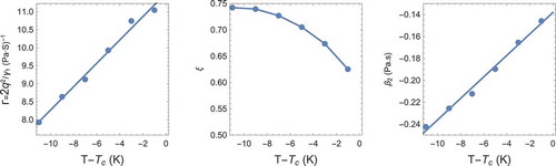
One interesting observation from the fits is that the isotropic viscosity $\eta$ is very small compared to the other viscosity coefficients. Even in the isotropic phase the shear viscosity is dominated by the orientational relaxation time. Unlike the elastic constants where the temperature dependence was primarily due to the order parameters variation in temperature, the viscosity coefficients $\mathrm{\Gamma }$, $\xi$, and ${\beta }_2$ do depend on temperature in Figure 4. Whether this could be eliminated by a somewhat different choice of coefficients is not entirely clear (for instance a different choice of what is a flux and what is a force in Equation (24)(24) $\begin{array}{rl}& T\dot{S}=\frac{d{Q}_{\alpha \beta }}{dt}{H}_{\alpha \beta }+{\sigma }_{\alpha \beta }^s{D}_{\alpha \beta }+{\tau }_{\alpha \beta }{\mathrm{\Omega }}_{\alpha \beta },\\ & =\frac{\delta Q_{\alpha \beta }}{\delta t}{H}_{\alpha \beta }+{\sigma }_{\alpha \beta }^s{D}_{\alpha \beta }.\end{array}$(24) ) but would be worthwhile to investigate.

3. Modelling surfaces and objects in a liquid crystal

One option to model the surface of a liquid crystal would be to impose boundary conditions for $Q_{\alpha \beta }$. One problem with doing this is that disclinations (topological defects in the field) often accompany interfaces, especially if they are curved, and these defects are often pinned to or terminate on a surface. Imposing fixed values of $Q_{\alpha \beta }$ on the surface may make this hard to occur. An alternative is to impose a surface free energy contribution to $\mathcal{F}$,

(50) $\int F_{s}dS,$(50)

with $F_s$ chosen so that its minimum gives the desired boundary condition. In most work, the preferred director orientation on a surface is either normal or planar anchoring. The strength of the anchoring is controlled via a parameter ${\alpha }_s$. Typically one uses a large enough value of ${\alpha }_s$ to ensure that the surface director is along the desired direction almost everywhere except near topological defects that interact with the surface (this is referred to as ‘strong anchoring’). The desired planar or normal anchoring on the surface can be induced by $F_s$ of the form:

(51) $F_s=\frac{{\alpha }_s}{2}(Q_{\alpha \beta }-Q_{\alpha \beta }^0{)}^2\to \mathrm{N}\mathrm{o}\mathrm{r}\mathrm{m}\mathrm{a}\mathrm{l}\mathrm{a}\mathrm{n}\mathrm{c}\mathrm{h}\mathrm{o}\mathrm{r}\mathrm{i}\mathrm{n}\mathrm{g}.$(51)

(52) $F_s=\frac{{\alpha }_s}{2}({\tilde{Q}}_{\alpha \beta }-Q_{\alpha \beta }^{\mathrm{\perp }}{)}^2\to \mathrm{P}\mathrm{l}\mathrm{a}\mathrm{n}\mathrm{a}\mathrm{r}\mathrm{a}\mathrm{n}\mathrm{c}\mathrm{h}\mathrm{o}\mathrm{r}\mathrm{i}\mathrm{n}\mathrm{g},$(52)

where

(53) $Q_{\alpha \beta }^0=q_0({\hat{n}}_{\alpha }^0{\hat{n}}_{\beta }^0-\frac{1}{3}{\delta }_{\alpha \beta }),$(53)

(54) ${\tilde{Q}}_{\alpha \beta }=Q_{\alpha \beta }+\frac{1}{3}{\delta }_{\alpha \beta },$(54)

(55) $Q_{\alpha \beta }^{\mathrm{\perp }}=({\delta }_{\alpha \gamma }-{\hat{n}}_{\alpha }^0{\hat{n}}_{\gamma }^0)Q_{\gamma \nu }({\delta }_{\nu \beta }-{\hat{n}}_{\nu }^0{\hat{n}}_{\beta }^0),$(55)

and ${\stackrel{\mathbf{ˆ}}{\mathbf{n}}}^0$ is the surface normal, and $q_0$ is the equilibrium bulk value of $q$. Equation (55)(55) $Q_{\alpha \beta }^{\mathrm{\perp }}=({\delta }_{\alpha \gamma }-{\hat{n}}_{\alpha }^0{\hat{n}}_{\gamma }^0)Q_{\gamma \nu }({\delta }_{\nu \beta }-{\hat{n}}_{\nu }^0{\hat{n}}_{\beta }^0),$(55) is the projection of ${\tilde{Q}}_{\alpha \beta }$ onto the tangent plane of the surface [40].

3.1. Forces on the immersed object

In many simulations, the immersed object is held fixed and the liquid crystal is then just allowed to evolve around this fixed position. However, in a more realistic picture, the object will move in response to the liquid crystal configuration and one must model the forces responsible in order to describe this motion. One coupling between the fluid and immersed object arise from the hydrodynamic forces that occur when the particle moves through the liquid crystal. These forces occur due to the no-slip/no-flow boundary condition at the objects surface (i.e. the fluid velocity and particle velocity should match at the surface). Obtaining forces from this boundary condition can be done in a number of ways. One that is fairly straightforward to implement has its origins in the Debye-Bueche-Brinkman (DBB) model [41–43]. Here, the presence of the particle in the fluid is characterized by the force density,

(56) $\mathbf{f}=\gamma n(\mathbf{r})(\mathbf{v}-\mathbf{u}),$(56)

where the coupling constant $\gamma$ has units of mass per time, $\mathbf{v}$ is the local velocity of the particle at the point $\mathbf{r}$, and $\mathbf{u}$ is the fluid velocity at the same point. The ‘node’ density $n(\mathbf{r})$, with units of inverse volume, is normally considered to be constant inside the particle, and zero outside. This force density is added to the right-hand side of Navier-Stokes Equation (31)(31) $\rho ({\mathrm{\partial }}_t+u_{\beta }{\mathrm{\partial }}_{\beta })u_{\alpha }={\mathrm{\partial }}_{\beta }{\sigma }_{\alpha \beta }^s+{\mathrm{\partial }}_{\beta }{\sigma }_{\alpha \beta }^e+{\mathrm{\partial }}_{\beta }{\tau }_{\alpha \beta },$(31) and provides the force of the particle on the fluid. This model was originally designed to model porous particles where the mean pore size ${\kappa }^{-1}\sim \sqrt{\eta /(\gamma n)}$ where $\eta$ is the fluid viscosity. In the limit of large $\gamma$ and/or large $n$, the no-slip/no-flow boundary condition is recovered [44,45]. It is also straightforward to deduce the force on the particle directly from Newton’s third law by integrating $-\mathbf{f}$ over a volume of the particle to get the local force on that volume. This accounts for the forces due to the fluid and particle motion, but not the forces due to the liquid crystal boundary condition. These are not included in this calculation and are dealt with separately.

The effect of the particle presence on the liquid crystal is already accounted for via the surface conditions Equation (52)(52) $F_s=\frac{{\alpha }_s}{2}({\tilde{Q}}_{\alpha \beta }-Q_{\alpha \beta }^{\mathrm{\perp }}{)}^2\to \mathrm{P}\mathrm{l}\mathrm{a}\mathrm{n}\mathrm{a}\mathrm{r}\mathrm{a}\mathrm{n}\mathrm{c}\mathrm{h}\mathrm{o}\mathrm{r}\mathrm{i}\mathrm{n}\mathrm{g},$(52) . However, liquid crystals are capable of transmitting forces and local torques even in cases when there is no flow in the system [8]. These effects are not well represented by Equation (56)(56) $\mathbf{f}=\gamma n(\mathbf{r})(\mathbf{v}-\mathbf{u}),$(56) . In this case, the local force that the fluid outside exerts on the particle can be described via [46]

(57) $d{F}_{\alpha }={\sigma }_{\alpha \beta }^{eq}d{S}_{\beta },$(57)

where the surface area element $\mathbf{d}\mathbf{S}$ points along the unit normal pointing out and ${\sigma }^{eq}$ is the equilibrium stress tensor in the fluid (dissipative terms are accounted for via Equation (56)(56) $\mathbf{f}=\gamma n(\mathbf{r})(\mathbf{v}-\mathbf{u}),$(56) and should not be included here or one will be double counting). It is important for the implementation of this force to note that Equation (57)(57) $d{F}_{\alpha }={\sigma }_{\alpha \beta }^{eq}d{S}_{\beta },$(57) is evaluated on the outside of the surface. While these local forces can result in a net torque on the immersed object, it can also experience a torque due to the $Q$-field itself via the equilibrium contributions to the anti-symmetric stress $\tau$ in Equation (23)(23) ${\tau }_{\alpha \beta }=Q_{\alpha \gamma }{H}_{\gamma \beta }-H_{\alpha \gamma }{Q}_{\gamma \beta }.$(23) . This produces a local torque on a volume element $dV$ of

(58) ${\mathrm{\Gamma }}_{\alpha }=2{\tau }_{\beta \gamma }dV,$(58)

where $\alpha$, $\beta$, $\gamma$ are a cyclic permutation of $x$, $y$, and $z$.

4. Algorithms

The earliest examination of colloids in liquid crystals involved approximations based on the Ericksen-Leslie equations being reduced to poisson-like equations and then using an image-charge method [1,47]. Computer simulation of colloids in liquid crystals using a tensor order parameter started with direct minimization of the liquid crystal free energy for a fixed configuration of colloids [48].

Even if the only thing desired is a steady-state or equilibrium configuration, it can be worthwhile to simulate the full dynamics. This is due to the myriad possible local minima that can arise from slightly different configurations of the topological defect lines. The ability to arrive at a minima of the free energy in some consistent manner using realistic dynamics leads to more confidence that such a configuration may be observed in an actual experiment. The dynamics involve two parts: the evolution of the fluid mass/momentum and the evolution of the LC order parameter.

4.1. Hybrid schemes for the fluid evolution

The lattice Boltzmann algorithm is a widely used method for simulating fluids. Its advantage is that it is fairly straightforward to code, is highly efficient, and it is a mass and momentum conserving algorithm. Its disadvantage is that it requires more memory than, say a finite-difference method that directly solves Navier-Stokes, as it replaces the four component partial differential equations (continuity equation for mass density and 3-component equations for evolution of the momentum density) with a set of 15 or more equations of the form:

(59) $({\mathrm{\partial }}_t+e_{i\alpha }{\mathrm{\partial }}_{\alpha })f_i=-\frac{1}{{\tau }_f}(f_i-f_i^{eq})+p_i.$(59)

The $f_i$ here are known as partial distribution functions $f_i=f_i(\mathbf{x},\mathbf{t})$ and describe the set of particles that are moving along a number of discrete velocity directions ${\mathbf{e}}_i$. (These velocities are chosen to take the $f_i$ to a neighboring lattice site in the time step $\mathrm{\Delta }t$). The ${\tau }_f$ is a relaxation time, $p_i$ are addition forces from either the colloidal particles or the liquid crystal degrees of freedom, and $f_i^{eq}$ is the equilibrium distribution function.

The fluid density $\rho$ and velocity $\mathbf{u}$ are related to the moments of the distribution function, i.e.

(60) $\rho \equiv \sum _i{f}_i;\rho \mathbf{u}\equiv \sum _i{f}_i{\mathbf{e}}_i.$(60)

The $f_i^{eq}$ can be expressed as Maxwell-Boltzmann-like distributions expanded assuming low velocities (relative to the speed of sound) and are constructed to ensure the moments in Equation (60)(60) $\rho \equiv \sum _i{f}_i;\rho \mathbf{u}\equiv \sum _i{f}_i{\mathbf{e}}_i.$(60) are conserved. Thus, the $f_i^{eq}$ depend on the local density and the fluid velocity. In addition, the second moment of the distribution function is related to the symmetric part of the stress tensor in the system (which is imposed on the second moment of the equilibrium distribution $f_i^{eq}$). As a result, the fluid picks up the coupling to the local order parameter $Q$ [39,45,49,50]. The effect of the anti-symmetric part of the stress tensor (Equation (23)(23) ${\tau }_{\alpha \beta }=Q_{\alpha \gamma }{H}_{\gamma \beta }-H_{\alpha \gamma }{Q}_{\gamma \beta }.$(23) ) is computed via a force density incorporated in the $p_i$.

One can solve Equation (59)(59) $({\mathrm{\partial }}_t+e_{i\alpha }{\mathrm{\partial }}_{\alpha })f_i=-\frac{1}{{\tau }_f}(f_i-f_i^{eq})+p_i.$(59) numerically a number of different ways. Typically, one starts with a cubic lattice and then replace the left-hand side with

(61) $\frac{f_i({\mathbf{r}}_{\mathbf{m}}+{\mathbf{e}}_i\mathrm{\Delta }t,t+\mathrm{\Delta }t)-f_i({\mathbf{r}}_{\mathbf{m}},t)}{\mathrm{\Delta }t}$(61)

at lattice site $\mathbf{m}$ at location ${\mathbf{r}}_{\mathbf{m}}$. The right-hand side of Equation (59)(59) $({\mathrm{\partial }}_t+e_{i\alpha }{\mathrm{\partial }}_{\alpha })f_i=-\frac{1}{{\tau }_f}(f_i-f_i^{eq})+p_i.$(59) is then evaluated at $({\mathbf{r}}_{\mathbf{m}},t)$. The resulting equation can then be solved for $f_i({\mathbf{r}}_{\mathbf{m}}+{\mathbf{e}}_i,t+\mathrm{\Delta }t)$ in terms of quantities evaluated at the previous time-step. While at first glance it appears that this Euler-like scheme would be only first order in $\mathrm{\Delta }t$, it can be shown that it is, in fact, equivalent to a second-order trapezoidal scheme [51]. One difficulty that arises for liquid crystals is that it is tricky to get the standard algorithm to match up with a second-order scheme for the evolution of the liquid crystal. A number of different alternative integration schemes for the lattice-Boltzmann equation have been proposed to help deal with this, including a predictor-corrector scheme [39] and exponential integrator [52].

One can also construct a lattice-Boltzmann-like scheme for the liquid crystal evolution using an evolution equation

(62) $({\mathrm{\partial }}_t+e_{i\alpha }{\mathrm{\partial }}_{\alpha }){\mathbf{G}}_i=-\frac{1}{{\tau }_G}({\mathbf{G}}_i-{\mathbf{G}}_i^{eq})+{\mathbf{M}}_i,$(62)

where ${\tau }_G$ is a relaxation parameter, ${\mathbf{M}}_i$ is an additional force required to recover the macroscopic equations, and the order parameter is related to the first moment of the ${\mathbf{G}}_i$:

(63) $Q_{\alpha \beta }=\sum _i{G}_{\alpha \beta ,i}.$(63)

This is then integrated using the same scheme as Equation (59)(59) $({\mathrm{\partial }}_t+e_{i\alpha }{\mathrm{\partial }}_{\alpha })f_i=-\frac{1}{{\tau }_f}(f_i-f_i^{eq})+p_i.$(59) . In this case, this requires a large number of finite-difference approximations in order to evaluate all of the derivative terms that appear in the equations of motion. This makes the evaluation of ${\mathbf{G}}_i^{eq}$ quite expensive. As a result, schemes that favor one evaluation of ${\mathbf{G}}_i^{eq}$ per time step, such as an exponential integrator, are favored over ones that require two evaluations, such as predictor-corrector schemes. However, as the order parameter itself is not actually a conserved quantity, nor are any of its moments, the advantages of using a lattice-Boltzmann-like scheme for the evolution of $\mathbf{Q}$ are somewhat limited. There is also the considerable storage cost associated with storing 15 or more ${\mathbf{G}}_i$. This coupled with the fact that, in order to get it to work, most of the evolution equations need to be computed via finite-differences anyway, some researchers just use a finite-difference scheme for $Q_{\alpha \beta }$ directly [53].

4.2. Object representation and coupling

To simulate objects in the liquid crystal we start with the hybrid lattice Boltzmann scheme described above for the fluid. This fluid exists on a discrete mesh. Our object must also be discretized into a set of nodes, typically on its surface, as illustrated in Figure 5. However, these surface nodes will not typically coincide with the mesh sites of the liquid. This implies that the effect of the surface nodes must be distributed to the nearest fluid mesh sites using some scheme to determine what weights an additional surface field, such as those in Equations (56)(56) $\mathbf{f}=\gamma n(\mathbf{r})(\mathbf{v}-\mathbf{u}),$(56) , (57(57) $d{F}_{\alpha }={\sigma }_{\alpha \beta }^{eq}d{S}_{\beta },$(57) ), and (58(58) ${\mathrm{\Gamma }}_{\alpha }=2{\tau }_{\beta \gamma }dV,$(58) ), represented at the surface nodes has to be added to these sites. Conversely, forces from the liquid crystal that affect the object are calculated at the fluid mesh sites and then interpolated with the same scheme to be applied to the node of the object as a weighted sum.

Figure 5. Schematic in 2 dimensions of the fluid mesh (black) sites ${\mathbf{r}}_{\mathbf{m}}$ and surface node (blue) sites $r_{\alpha }$ that represent the object.

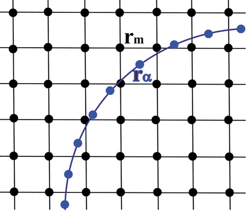
To accurately model these surface forces one needs to consider a number of factors. First, in order to prevent the fluid from penetrating the object, the surface nodes need to be slightly less than $\mathrm{\Delta }x$ (the fluid mesh spacing) apart. There is, however, no need to be significantly closer than this as it is not likely to improve the accuracy while coming with greater computation cost.

A number of interpolation schemes can be used to distribute the nodes to fluid mesh (and vice versa). One might think that spreading the force over more mesh sites will lead to significantly higher accuracy. However, due to the singular nature of the boundary forces, this can make the effective size of the object somewhat larger. A more compact interpolation scheme, such as from using a trilinear stencil, can alleviate this somewhat. We label each node of the object with an index $\alpha$ and its coordinates by ${\mathbf{r}}_{\alpha }=(x_{\alpha },y_{\alpha },z_{\alpha })$. This node is located inside a cubic (in 3D) cell of the fluid mesh and thus has eight mesh sites around it. These fluid mesh sites are indexed by $m\in [\mathrm{0..7}]$ and have coordinates ${\mathbf{r}}_m=(x_m,y_m,z_m)$. The scaled difference along the axes between the mesh site and object node, $(x_{m\alpha },y_{m\alpha },z_{m\alpha })\equiv ({\mathbf{r}}_m-{\mathbf{r}}_{\alpha })/\mathrm{\Delta }x$ is then used to compute the weights from the nodes $\alpha$ at site $m$,

(64) ${\zeta }_{m\alpha }=\psi (x_{m\alpha })\psi (y_{m\alpha })\psi (z_{m\alpha })$(64)

where $\psi$ for the trilinear interpolation stencil is defined by,

(65) $\psi (w)=1-|w|.$(65)

These weights satisfy ${\sum }_m{\zeta }_{m\alpha }=1$ and can be used as weights to get the interpolated value of something on the fluid mesh at the node $\alpha$ (for example, the fluid velocity at the object surface). Other weighting schemes that go further than one $\mathrm{\Delta }x$ from the object node are also possible and there are advantages and disadvantages to different schemes [45,54]. Newton’s third law typically requires that the same weights be used to transfer an equal and opposite force onto the object as was transferred to the fluid mesh from the object. If there are more than one node in a cubic cell, then the weights from each node contribute to the forces at each fluid mesh site [45,54].

To model a spherical colloid, a surface triangulation of nodes can be used. Alternatively, molecular fullerenes with anywhere from 20 to several thousand atoms (which become the surface nodes) are available. To model rods, it is generally best to use something resembling a twisted multi-stranded rope [55] which works better than a straight string of nodes as the twist significantly reduces undesirable commensurability effects with the lattice mesh at orientations that match the coordinate directions of the mesh.

Edge and end effects can also be problematic. As in electrostatics, where edges can be places where charge accumulates, edges and ends can cause the generation of topological defects. However, care must be taken when enforcing a strict boundary condition as this will almost certainly generate a defect. However, in reality, a liquid crystal system can often ‘heal’ such a defect as long as the end or edge of the object induces an effect that has a smaller scale than the correlation length of order in the liquid crystal (which might be quite large). Imposing the boundary conditions via a somewhat softer potential, such as in Equation (56)(56) $\mathbf{f}=\gamma n(\mathbf{r})(\mathbf{v}-\mathbf{u}),$(56) , or leaving it free at the edge often leads to better agreement with experiments [52].

5. Small objects by themselves

Analytic calculations are few and far between in this field. However, there are a few calculations that can be made for certain single objects in a liquid crystal. In addition to their inherent usefulness, they can also be valuable for validation of the simulation technique. These are most easily done in cases where the object shape is compatible (at least in equilibrium) with the liquid crystal as they do not have defects (disclination lines) associated with them.

For the analytic calculation, we start with the Frank elastic energy, Equation (8)(8) ${\mathcal{F}}_d=\int d\mathbf{r}\left[\frac{1}{2}{K}_1{(\mathrm{\nabla }\cdot \mathbf{n})}^2+\frac{1}{2}{K}_2{(\mathbf{n}\cdot \mathrm{\nabla }\times \mathbf{n})}^2+\frac{1}{2}{K}_3{(\mathbf{n}\times \mathrm{\nabla }\times \mathbf{n})}^2\right].$(8) , and in the approximation where all the elastic constants are equal. The director is a unit length vector and it is easiest to impose this constraint if we take $\stackrel{\mathbf{ˆ}}{\mathbf{n}}=(cos\theta sin\varphi ,sin\theta sin\varphi ,cos\varphi )$. Note that $\theta$ and $\varphi$ are the local azimuthal and polar angles of the director and, in general depend on location $\mathbf{r}$. In terms of $\theta$ and $\varphi$ the Frank free energy can then be written as

(66) $F_{el}=\frac{1}{2}K[(\mathrm{\nabla }\varphi {)}^2+(\mathrm{\nabla }\theta {)}^2{sin}^2\varphi +2n\cdot (\mathrm{\nabla }\theta \times \mathrm{\nabla }\varphi )sin\varphi ].$(66)

Minimizing this yields two coupled Euler-Lagrange equation [56]

${\mathrm{\nabla }}^2\varphi -sin\varphi cos\varphi (\mathrm{\nabla }\theta {)}^2=0,$

(67) $sin\varphi {\mathrm{\nabla }}^2\theta +2cos\varphi \mathrm{\nabla }\varphi \cdot \mathrm{\nabla }\theta =0.$(67)

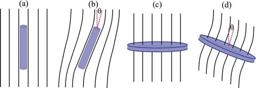
These equations are highly non-linear and further simplification is needed in order to solve them. There are some shapes, in particular a wire with tangential director boundary conditions or a disc with normal director boundary conditions, that have no distortion of the director field in equilibrium. Further, if we rotate these shapes by a small angle, no out-of-plane deformations occur. This is illustrated in Figure 6. In these cases, we can assume $\varphi$ is approximately constant and very close to $\pi /2$. With these assumptions, Equation (67)(67) $sin\varphi {\mathrm{\nabla }}^2\theta +2cos\varphi \mathrm{\nabla }\varphi \cdot \mathrm{\nabla }\theta =0.$(67) reduces simply to Laplace’s equation

(68) ${\mathrm{\nabla }}^2\theta =0.$(68)

Figure 6. Objects in a liquid crystal. The lines are tangential to the director field. (a) A thin wire in equilibrium. (b) A thin wire under external torque that twists it away from equilibrium. (c) Thin disk in equilibrium. (d) Thin disc under external torque that twists it away from equilibrium. In (b) and (d) the object experiences a counter-torque from the nematic field in the direction to decrease $\theta$.

For a wire, we now assume that it can be reasonably approximated as a prolate spheroidal shape, primarily because Laplace’s equation has an exact solution in a corresponding coordinate system. The appropriate coordinate change from cartesian $(x,y,z)$ to prolate-spheroidal coordinates $(s,t,\mathrm{\Xi })$ is defined by

(69) $s\equiv \frac{\sqrt{x^2+y^2+{(z+a)}^2}+\sqrt{x^2+y^2+{(z-a)}^2}}{2a}$(69)

(70) $t\equiv \frac{\sqrt{x^2+y^2+{(z+a)}^2}-\sqrt{x^2+y^2+{(z-a)}^2}}{2a}$(70)

(71) $\mathrm{\Xi }\equiv {tan}^{-1}\left(\frac{y}{x}\right),$(71)

where $a$ is the (constant) interfocal distance. We now assume that the boundary condition on the surface of the wire requires that the director be tangential to the surface and along the orientation of the wire. Laplace’s Equation (68)(68) ${\mathrm{\nabla }}^2\theta =0.$(68) then has the solution [57]

(72) $\theta ={\theta }_o\frac{ln\left(\frac{s+1}{s-1}\right)}{ln\left(\frac{s_o+1}{s_o-1}\right)},$(72)

where the constant $s_o$ defines the prolate spheroidal surface (similar to a radius for a sphere). From this, we can also compute the total Frank free energy (8), integrated over all space, as a function of the wire’s orientation ${\theta }_0$. As $\varphi$ is $\pi /2$, this becomes

(73) $U_{el}=\frac{K}{2}\int dV(\mathrm{\nabla }\theta {)}^2=2\pi CK{\theta }_0^2,$(73)

with $C$ being constant, and referred to as a capacitance in analogy to electrostatics. Making use of Equation (69)(69) $s\equiv \frac{\sqrt{x^2+y^2+{(z+a)}^2}+\sqrt{x^2+y^2+{(z-a)}^2}}{2a}$(69) , the capacitance is

(74) $C=a{\left[ln\frac{s_o+1}{s_o-1}\right]}^{-1}$(74)

(75) $=2L\sqrt{1-{\left(\frac{R}{L}\right)}^2}{\left[ln\left(\frac{1+\sqrt{1-{\left(\frac{R}{L}\right)}^2}}{1-\sqrt{1-{\left(\frac{R}{L}\right)}^2}}\right)\right]}^{-1},$(75)

where $R$ and $L$ are the radius and length of the wire, respectively. In the limit $\frac{R}{L}\to 1$ the capacitance is simply $C\to R$, that of a sphere, as expected. In the high aspect ratio limit, $\frac{R}{L}\to 0$, the capacitance is

(76) $C\approx \frac{L}{ln\left(\frac{2L}{R}\right)}.$(76)

Although Equation (76)(76) $C\approx \frac{L}{ln\left(\frac{2L}{R}\right)}.$(76) is the capacitance for a prolate ellipsoid, it can be used as a low order approximation to a long thin cylindrical object like a wire [55]. In this case, it is necessary to assume that the wire’s ends are small enough (smaller or comparable to the size of a disclination) that we can neglect the end effects (i.e. we do not require the director to be tangential to the flat ends of the cylinder). It is not possible to solve Laplace’s equation exactly for a cylinder, but expanding in $1/\zeta =1/ln(\frac{2L}{R})$, Jackson [58] derived an approximate expression,

(77) $\begin{array}{rl}& C=L\left\{\frac{1}{\zeta }+\frac{1}{{\zeta }^2}(1-ln2)\right.\\ & +\left.\frac{1}{{\zeta }^3}\left[1+{(1-ln2)}^2-\frac{{\pi }^2}{12}\right]+O(1/{\zeta }^4)\right\}.\end{array}$(77)

For high aspect ratio wires, both Equations (76)(76) $C\approx \frac{L}{ln\left(\frac{2L}{R}\right)}.$(76) and (77(77) $\begin{array}{rl}& C=L\left\{\frac{1}{\zeta }+\frac{1}{{\zeta }^2}(1-ln2)\right.\\ & +\left.\frac{1}{{\zeta }^3}\left[1+{(1-ln2)}^2-\frac{{\pi }^2}{12}\right]+O(1/{\zeta }^4)\right\}.\end{array}$(77) ) are equivalent. For low aspect ratio wires, there are significant differences between the two equations and Equation (77)(77) $\begin{array}{rl}& C=L\left\{\frac{1}{\zeta }+\frac{1}{{\zeta }^2}(1-ln2)\right.\\ & +\left.\frac{1}{{\zeta }^3}\left[1+{(1-ln2)}^2-\frac{{\pi }^2}{12}\right]+O(1/{\zeta }^4)\right\}.\end{array}$(77) should be used instead.

A similar calculation is possible for other coordinate systems in which Laplace’s Equation (68)(68) ${\mathrm{\nabla }}^2\theta =0.$(68) is separable [57]. For example, for an oblate spheroid (which can be used to approximate a disc [29,52]) with boundary condition that the director be perpendicular to the surface one can obtain a similar expression to (73). In this case, the angle $\theta$ is between the normal to the face of the disc or spheroid and the direction of the director at $\mathrm{\infty }$. This gives

(78) $C=\frac{L}{2}\sqrt{{\left(\frac{2R}{L}\right)}^2-1}{\left(arctan\left(\sqrt{{\left(\frac{2R}{L}\right)}^2-1}\right)\right)}^{-1},$(78)

where $R$ is the radius of the disc and $L$ is its thickness. Again, one must assume that the disc edge does not generate a defect, meaning that the disc must be quite thin for this to be valid.

Figure 7. Effective ‘capacitance’ (analogy to electrostatics) defined in Equation (73)(73) $U_{el}=\frac{K}{2}\int dV(\mathrm{\nabla }\theta {)}^2=2\pi CK{\theta }_0^2,$(73) of objects in a liquid crystal. (left) Wire shape (long thin cylinder) with tangential boundary conditions. The points are from a simulation [55], the solid line is from Equation (77)(77) $\begin{array}{rl}& C=L\left\{\frac{1}{\zeta }+\frac{1}{{\zeta }^2}(1-ln2)\right.\\ & +\left.\frac{1}{{\zeta }^3}\left[1+{(1-ln2)}^2-\frac{{\pi }^2}{12}\right]+O(1/{\zeta }^4)\right\}.\end{array}$(77) , the dashed line from Equation (76)(76) $C\approx \frac{L}{ln\left(\frac{2L}{R}\right)}.$(76) , and the dotted line from Equation (75)(75) $=2L\sqrt{1-{\left(\frac{R}{L}\right)}^2}{\left[ln\left(\frac{1+\sqrt{1-{\left(\frac{R}{L}\right)}^2}}{1-\sqrt{1-{\left(\frac{R}{L}\right)}^2}}\right)\right]}^{-1},$(75) . (right) Disc shape (short fat cylinder) with normal boundary conditions. The points are from a simulation [52] and the line is from Equation (78).

Figure 7 shows the results of simulations on a wire [55] and a disc [52] and the predictions of Equations (75)(75) $=2L\sqrt{1-{\left(\frac{R}{L}\right)}^2}{\left[ln\left(\frac{1+\sqrt{1-{\left(\frac{R}{L}\right)}^2}}{1-\sqrt{1-{\left(\frac{R}{L}\right)}^2}}\right)\right]}^{-1},$(75) , (76(76) $C\approx \frac{L}{ln\left(\frac{2L}{R}\right)}.$(76) ), (77(77) $\begin{array}{rl}& C=L\left\{\frac{1}{\zeta }+\frac{1}{{\zeta }^2}(1-ln2)\right.\\ & +\left.\frac{1}{{\zeta }^3}\left[1+{(1-ln2)}^2-\frac{{\pi }^2}{12}\right]+O(1/{\zeta }^4)\right\}.\end{array}$(77) ), and (78(78) $C=\frac{L}{2}\sqrt{{\left(\frac{2R}{L}\right)}^2-1}{\left(arctan\left(\sqrt{{\left(\frac{2R}{L}\right)}^2-1}\right)\right)}^{-1},$(78) ). As we can see from the plots, the spheroidal shapes give a reasonable qualitative description of the effective capacitance of cylindrical but to get an accurate measure one needs to use a more systematic expansion for a cylinder unless $R/L$ is quite small.

The approximations required for these calculations do not hold when the object is twisted to a large angle $\theta$. At this point, the energy can be decreased by moving out of plane and the object spontaneously ‘flips’ [52,59,60]. We will discuss this further in a later section.

Most particles immersed in a liquid crystal with strong anchoring at their surface will induce a corresponding defect in the nematic field to compensate for their topological charge. This was first reported by Meyer [1] in 1972 where the main interest at that time was the existence of an actual point defect rather than a disclination line. The analogy to electrostatics and the use of the image charge technique within the Ericksen-Leslie formalism were exploited in Ref [47] to account for the interaction of the cavity and the defect.

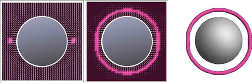
Figure 8. Cross-sections through the poles (left) and equator (middle) of a sphere in a nematic with normal anchoring. The color indicates the largest eigenvalue and the director field in the cross-section is shown in the left and middle plots (The length of the director is fixed. When they appear to get shorter they are pointing out of the plane). The right plot is a contour plot in 3-dimensions of the largest eigenvalue of $\mathbf{Q}$ looking down on the sphere from above.

Until recently, very few analytical results were available that were based on the tensor order parameter. However, this may have been due to the unwarranted assumption that any such description would be necessarily intractable. Recent work has shown this to not be the case [61–64]. In fact, in the one elastic constant approximation, they found a solution for small spheres in a nematic with normal boundary conditions [61]

(79) $\mathbf{Q}\approx \frac{w}{3+w}{\left(\frac{a}{r}\right)}^3{\mathbf{Q}}^0+\left(1-\frac{w}{1+w}\frac{a}{r}\right){\mathbf{Q}}^{\mathrm{\infty }}$(79)

where $a$ is the sphere radius, $w=2a{\alpha }_s/L_1$, ${\mathbf{Q}}^0$ is given in Equation (53)(53) $Q_{\alpha \beta }^0=q_0({\hat{n}}_{\alpha }^0{\hat{n}}_{\beta }^0-\frac{1}{3}{\delta }_{\alpha \beta }),$(53) , and ${\mathbf{Q}}^{\mathrm{\infty }}$ is the order parameter far from the sphere. There are no obvious singularities in this field (outside the sphere). There is however a Saturn-ring disclination [2,3,65] looping around the equator of the sphere. In the tensor order parameter, this Saturn defect appears as an eigenvalue exchange [66] and the principal eigenvector becomes discontinuous. The location of the defect ring can be found as a root of a cubic polynomial. For strong anchoring, the ring is well separated from the sphere but as the anchoring strength ${\alpha }_s$ is decreased, the ring collapses onto the spheres surface [61]. Far from the sphere, the principal eigenvector of the expression in Equation (79)(79) $\mathbf{Q}\approx \frac{w}{3+w}{\left(\frac{a}{r}\right)}^3{\mathbf{Q}}^0+\left(1-\frac{w}{1+w}\frac{a}{r}\right){\mathbf{Q}}^{\mathrm{\infty }}$(79) can be computed and is found to be

(80) ${\mathbf{n}}^0=\stackrel{\mathbf{ˆ}}{\mathbf{z}}+\frac{w}{3+w}\frac{a^3}{r^5}(xz,yz,0)+O\left({\left(\frac{a}{r}\right)}^4\right),$(80)

a quadrupolar far-field behavior predicted from an electrostatic analogy [67]. For large spheres [62], the ring is replaced with a point defect above one of the poles. This is the so-called dipole configuration, named for the far-field behavior, again in analogy to electrostatics.

The results of a simulation of a sphere in a nematic with the director anchored normal to its surface are shown in Figure 8. The far-field director is aligned with the axis of the sphere. One can readily see that the presence of the disclination line very effectively confines the distortion in the director field to a distance not significantly larger than the disclination’s radius. The principal eigenvalue dips down before crossing at the disclination core which makes it fairly straightforward to identify the defect. In the later plots, we will primarily show just a contour plot of the largest eigenvalue (the plot on the right in Figure 8).

Figure 9. Far-field director configuration (bar on left) and disclination lines around a sphere with normal anchoring conditions for the director in a cholesteric liquid crystal. As the pitch of the cholesteric gets shorter (going from (a) to (e)) the disclination twists around the sphere to match.

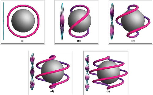
In a colloid-free cholesteric liquid crystal in its equilibrium state, the system breaks symmetry and picks a direction for an axis about which it will exhibit a twist. The pitch of the cholesteric twist can be tuned using different techniques. For example, often a cholesteric can be produced by doping a nematic with a small concentration of chiral molecules. Figure 9 shows what happens to a colloid with a saturn-ring defect when placed in a cholesteric as we vary the pitch [68–70]. In this case, the director is still always perpendicular to the surface but the disclination loop twists around the sphere with the number of twists being the same as the ratio of the sphere diameter to the pitch of the cholesteric.

Figure 10. Far-field director configuration (bars on left of subfigures) and (a-d) disclination lines around a sphere with tangential anchoring conditions in a cholesteric liquid crystal. (e) and (f) show the director configuration on the surface of the sphere for (a) and (c) respectively.

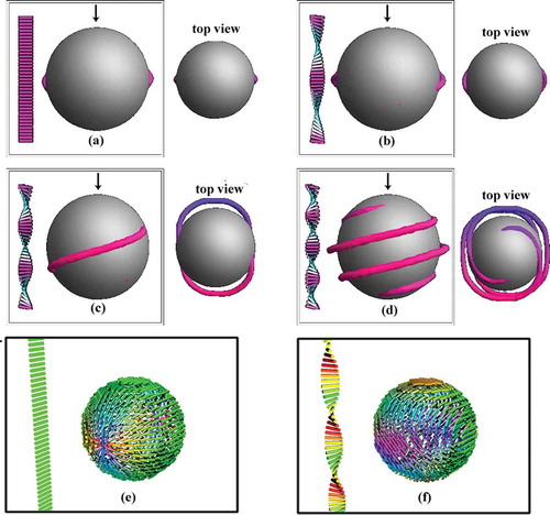
At first glance, the situation of a sphere with tangential anchoring for the director on the surface of the sphere looks similar, as illustrated in Figure 10(a-d). If not already split, the $+1$ defect at the poles of the sphere in the nematic (Figure 10(a) and (e)) splits into a $+1/2$ defect line with both ends terminating on the surface near the poles. As with the sphere with normal anchoring, as the pitch of the cholesteric becomes tighter, the disclination line twists around the sphere with the number of twists being proportional to the ratio of the sphere diameter to the pitch of the cholesteric. However, when we examine the director configuration on the surface of the sphere (Figure 10(e) and (f)) we see that even though the director remains tangential to the surface its configuration changes dramatically in the cholesteric. It weaves around on the surface similar to the stitch on a baseball in Figure 10(f). This variability in the surface director makes it somewhat more difficult to obtain an analytic solution similar to Equation (79)(79) $\mathbf{Q}\approx \frac{w}{3+w}{\left(\frac{a}{r}\right)}^3{\mathbf{Q}}^0+\left(1-\frac{w}{1+w}\frac{a}{r}\right){\mathbf{Q}}^{\mathrm{\infty }}$(79) as the director configuration on the surface is not known a-priori.

6. Configurations of multiple objects

Figure 11. (a) Spheres with tangential anchoring in a cholesteric where the pitch is comparable to the sphere diameter (as in Figure 10c & f) are ‘bonded’ by disclination lines. (b) The energy of a pair of these colloids as a function of their separation shows a distinct change when the disclination lines bonding the particles breaks. Data used in this plot is from Ref [69].

When multiple colloids are placed in the liquid crystal a variety of structures form, including chains and clusters [48,71–76]. Fig. 11 illustrates a case of a ‘bonded’ chain of colloids in a cholesteric liquid crystal [69]. In this case, the pitch of the cholesteric is comparable to that of the sphere diameter, similar to the single colloid case illustrated in Figure 10(c) and f. As shown in that figure, when the colloids are well separated, they have two handles near the poles formed by $+1/2$ disclination lines whose ends attach to the sphere’s surface. When the spheres are brought close together these handles break and instead form a direct ‘bond’ to the neighboring colloid. These are very close to an ideal harmonic bond as illustrated by the quadratic dependence of the bond energy versus the colloid separation (as illustrated in Figure 11(b)). However, as the bond length is increased, it eventually breaks which results in a discontinuous jump in the energy versus separation and a very different behavior of the particles versus distance at larger separations. This discontinuous behavior is not experienced by particles in a nematic with no bonding regime [77].

With strong normal anchoring, the attractive forces between two spherical colloids are oscillatory functions of particle separation and can be controlled through the chirality of the medium. The interaction between the particles is strongest at a pitch equal to the particle diameter and decreases as the chirality is increased further [78].

Figure 12. An example of a low energy configuration of two particles with different boundary conditions (the one on the left with director normal to the surface and the one on the right with the director tangential to the surface) in a cholesteric with pitch slightly smaller than the diameter of the sphere. The simulation results are from Ref [30].

Mixtures of spherical particle with normal and tangential boundary conditions have also been examined [30,79]. In a nematic, particles pair up (with a particle with opposite boundary conditions) and then typically organize themselves into a plane in either linear chains or into a 2D square lattice. When the medium is changed to a cholesteric, the result depends on the pitch. Systems with pitches larger than the particle size are fairly similar to a nematic except with slightly more winding of the saturn-ring type defects. In cases with a cholesteric pitch smaller than the particle size, the disclination lines are more likely to attach to a particle of opposite type and produce more complex patterns, an example of which is shown in Figure 12. In this case, there are multiple local minima in the binary pair interaction energy and not all of these are in the same plane [30]. This suggests that a number of complex structures could be formed from these sorts of particle mixtures.

7. Crystal structures

In addition to small clusters of colloids and linear chains, two-dimensional crystal structures have been observed in nematic emulsions [79,80]. Optical guiding by laser tweezers has been used to produce a variety of two and three-dimensional particle assemblies in cholesteric liquid crystals [81].

More exotic liquid crystal-colloid mixtures can lead to a variety of structures [82]. Using a blue-phase liquid crystal as the medium (similar to a cholesteric except the director twists along multiple axes) typically results in a 3D disclination network. By adding colloids to such a medium, the colloidal particles can be attracted to the disclination lines leading to stable close-packed three-dimensional crystals [83]. Further varieties of structures can be obtained by adjusting the anchoring strength at the colloid surface [84]. Colloids with binary boundary conditions (similar to those in Figure 12) in a cholesteric have a stable closed-packed body-centered cubic crystal structure [85] with the most stable structure having a pitch value such that the director would be expected to twist by $\pi$ over one unit cell of the lattice with minimal spacing between the colloids. Similar colloids in a nematic favor a face-centered cubic lattice structure [85].

One of the main reasons liquid crystals are useful in devices is due to their optical activity. As a result, it is worthwhile to consider if a colloidal crystal in a liquid crystal medium would exhibit interesting photonic structure. The periodicity of the dielectric constant in a photonic crystal gives them the ability to affect the propagation of photons due to the refraction and reflection of light at the many different interfaces in the system. One way to characterize this behavior is through the photonic band structure of the crystal. As in atomic crystals, non-closed packed crystal lattices are required to exhibit a band gap, similar to electrons in a semiconductor, where in this case, a certain range of frequencies of light cannot be propagated inside the periodic lattice [86]. For example, a diamond lattice structure of spheres with a different dielectric constant than the background material can have a complete band gap whereas a face-centered (close-packed) lattice structure will not [87]. It is therefore of interest to see if a stable colloidal crystal in a diamond lattice can be found in a liquid crystal medium.

Figure 13. Colloidal particles of diameter 1.1 µm in a cholesteric liquid crystal with a pitch of 5.5 µm arranged into a stable diamond lattice with 0.25 µm spacing between the colloids. The associated disclination lines are shown (colored lines). The top panel shows the view in the crystal from various viewpoints. The middle panel shows a single colloid in the crystal from the same viewpoints. The bottom panel shows just the disclination lines and the tetrahedral lattice structure connecting the centers of the colloids (the black lines). Data is from Ref [88].

It was shown that a locally stable diamond colloidal crystal can be obtained in a cholesteric in Ref [88]. The pitch must be tuned to match the crystal lattice spacing to get an energetically favorable crystal while having little or no separation between nearest-neighbor spheres. This is illustrated in Figure 13. In this case, the spheres have normal surface anchoring and the defect lines travel along the symmetry axes of the lattice. Stability of the lattice was demonstrated by examining the phonon frequency spectrum (for lattice vibrations). This crystal does exhibit a gap in its photonic band structure, as was demonstrated in Ref [89].

8. Dynamics

Particle dynamics are a more computationally challenging problem to study than static configurations. One of the difficulties that arise is that the response time of the fluid density is quite fast compared to the response time of the director field. However, they are far from being decoupled. The dynamics of the fluid flow affects the director orientation and the motion of the director causes ‘backflow’ in the fluid. This is not just a small quantitative shift but can have rather significant qualitative effects. For example, disclination lines experience a different drag force dependent on the direction of rotation of the director field going around the core and their direction of travel [90–93]. This is a result of the backflow created by the director and how it interacts with flow induced by the motion of the defect core.

A typical characterization of the dynamics of sphere in a simple fluid is the drag force required to pull the sphere through the fluid at a constant velocity. For low velocities, this force is typically linear in the velocity (Stokes drag), is directly proportional to the radius of the sphere, and directly opposes the forward velocity. However, this is not the case in a liquid crystal [94,95]. The drag is anisotropic and in some cases disclination lines can be shed from the moving sphere.

Figure 14. A magnetic disc rotating in a nematic liquid crystal. The director is normal to the two faces of the disc which are shown. The magnetic field is shown by the large arrow. At small angles the magnetic field is slightly ahead of the disc’s magnetic moment (which is in the plane of the disc) and the torque from the magnetic field is balanced by an equal and opposite torque the disc experiences from the liquid crystal from Equation (73)(73) $U_{el}=\frac{K}{2}\int dV(\mathrm{\nabla }\theta {)}^2=2\pi CK{\theta }_0^2,$(73) . The different frames, (a)-(i) represent different stages as the magnetic field is rotated through 180${ }^{\circ }$ and show the director field in a cross-section that goes through the center of the disc. The inset of each figure shows director ‘streamlines’ in three-dimensions in a region close to the disc. Frames (e)-(h) show where the director flips. These are not stable states and the disc flips continuously in time.

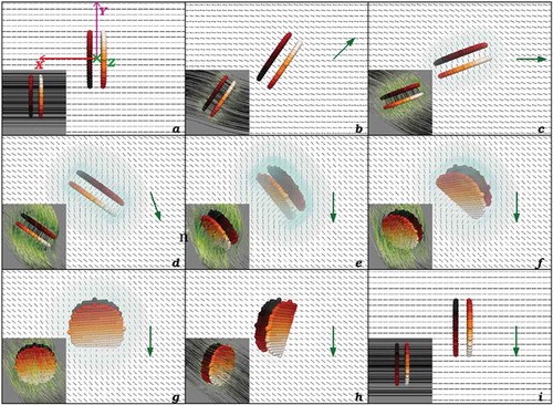
We now return to the case of the magnetic disc in a liquid crystal discussed in Section 5. In this case, the disc can be rotated within the liquid crystal by changing the external magnetic field [29,52,60]. When the disc is rotated to a high angle it becomes unstable and ‘flips’. This process is illustrated in Figure 14. This example illustrates some of the difficulties in comparing experiments and simulations. In an experiment the fact that one typically looks through the sample with crossed polarizers can make it look like there is a disclination present. For example in frames (f) and (g) in Figure 14, most of the director field is in the same plane except for a small region that will appear as a ring around the disc, similar to a disclination line, where the director field is normal to the plane. Simulations can clearly see that this ring is not a disclination. These insights can be very valuable for interpreting the results of experiments.

9. Conclusions and outlook

The understanding of colloids in liquid crystals has come a long way over the last few decades through improvements in theory, simulation, and experiments. There are still a wide variety of areas in need of further study. For example, flexible particles [96–98] and, by extension, swimmers in liquid crystals [99,100] are an emerging area of significant interest. There have been a number of recent works looking at how imperfections in the bulk of a liquid crystal can be used to organize assembly of colloids at an interface between the liquid crystal and isotropic phase [101–103]. To properly simulate such a system a two-phase fluid model with an interface between the fluids would be needed. As such interfaces can exhibit other fascinating properties, this could be an interesting line of study. The electroactivity of liquid crystals also opens up a variety of novel applications, such as particle sorting [104] and the effect of droplets on switching dynamics [105].

The one thing still lacking in the area of colloids in liquid crystals is the ‘killer’ application. It is often said that almost anything involving liquid crystals can, in principle, be turned into a device. Yet, the prime application of liquid crystals is still display devices and this remains the focus of most commercial activity. In this regards, perhaps what the field needs is more engineers or entrepreneurial scientists willing to take these ideas from the lab to the marketplace.

Acknowledgments

I would like to thank my current and former graduate students for their contributions to the work on this topic over many years and for agreeing to supply data and some figures for this review. In particular, I would like to thank Chris Smith, Frances Mackay, Alena Antipova, and Setareh Changizrezaei.

Disclosure statement

No potential conflict of interest was reported by the author.

Additional information

Funding

I would like to thank the Natural Science and Engineering Research Council of Canada (NSERC) for financial support. This research was enabled in part by support provided by Compute Ontario (http://www.computeontario.ca), WestGrid (http://www.westgrid.ca), and Compute Canada (http://www.computecanada.ca).

References

- Meyer RB. Point disclinations at a nematic-isotropic liquid interface. Mol Cryst Liq Cryst. 1972;16:355–40.
- Terentjev EM. Disclination loops, standing alone and around solid particles, in nematic liquid crystals. Phys Rev E. 1995 Feb;51:1330–1337.
- Gu Y, Abbott NL. Observation of saturn-ring defects around solid microspheres in nematic liquid crystals. Phys Rev Lett. 2000 Nov;85:4719–4722.
- Onsager L. The effects of shape on the interaction of colloidal particles. Ann N Y Acad Sci. 1949;51:627–659.
- Maier W, Saupe A. Eine einfache molekular-statistische theorie der nematischen kristallinflüssigen phase. teil l. Z Naturforschung A. 1959;14:882–889.
- Maier W, Saupe A. Eine einfache molekular-statistische theorie der nematischen kristallinflüssigen phase. teil ii. Z Naturforschung A. 1960;15:287–292.
- Humphries RL, James PG, Luckhurst GR. Molecular field treatment of nematic liquid crystals. J Chem Soc Faraday Trans 2. 1972;68:1031–1044.
- de Gennes P, Prost J. The physics of liquid crystals. 2nd ed. Oxford: Clarendon Press; 1993.
- Bunning JD, Crellin DA, Faber TE. The effect of molecular biaxiality on the bulk properties of some nematic liquid crystals. Liq Cryst. 1986;1:37–51.
- Karat P, Madhusudana N. Elastic and optical properties of some 4′-n-Alkyl-4-Cyanobiphenyls. Mol Cryst Liq Cryst. 1976;36:51–64.
- Dalmolen LGP, Picken SJ, de Jong AF, et al. The order parameters <P2> and <P4> in nematic p-alkyl-p’ -cyano-biphenyls: polarized Raman measurements and the influence of molecular association. J Phys France. 1985;46:1443–1449.
- Horn RG. Refractive indices and order parameters of two liquid crystals. J Phys France. 1978;39:105–109.
- Emsley J, Hamilton K, Luckhurst G, et al. Orientation order in the nematic phase of 4–methoxy–4ʹ–cyanobiphenyl: A deuterium NMR study. Chem Phys Lett. 1984;104:136–142.
- Fung BM, Poon CD, Gangoda M, et al. Nematic and smectic ordering in 4–n–octyl–4ʹ–cyanobiphenyl studied by carbon– 13 NMR. Mol Cryst Liq Cryst. 1986;141:267–277.
- Karat PP, Madhusudana NV. Orientational order and elastic constants of some cyanobiphenyls, part iii. Mol Cryst Liq Cryst. 1978;47:21–28.
- Bhattacharjee B, Paul S, Paul R. Orientational distribution function and order parameters of two 4ʹ–alkoxy–4–cyanobiphenyls in mesomorphic phase. Mol Cryst Liq Cryst. 1982;89:181–192.
- Limmer S, Schmiedel H, Hillner B, et al. Ordering and intramolecular mobility in the nematic phase of paa investigated by means of NMR lineshape analysis and computer simulations of the lineshape. J Phys France. 1980;41:869–878.
- Roy SK. Proton NMR studies in some cyano-biphenyls, oxy-cyano-biphenyls and paa at atmospheric pressure. J Phys II France. 1992;2:219–225.
- Jen S, Clark NA, Pershan PS, et al. Raman scattering from a nematic liquid crystal: orientational statistics. Phys Rev Lett. 1973 Dec;31:1552–1556.
- Heidenreich S, Ilg P, Hess S. Robustness of the periodic and chaotic orientational behavior of tumbling nematic liquid crystals. Phys Rev E. 2006 Jun;73:061710.
- Graziano DJ, Mackley MR. Disclinations observed during the shear of mbba. Mol Cryst Liq Cryst. 1984;106:103–119.
- Frank FC. I. liquid crystals. on the theory of liquid crystals. Discuss Faraday Soc. 1958;25:19–28.
- Beris AN, Edwards BJ. Thermodynamics of flowing systems. Oxford: Oxford University Press; 1994.
- Schiele K, Trimper S. On the elastic constants of a nematic liquid crystal. Phys Status Solidi B. 1983;118:267–274.
- Berreman DW, Meiboom S. Tensor representation of Oseen-Frank strain energy in uniaxial cholesterics. Phys Rev A. 1984 Oct;30:1955–1959.
- Chen GP, Takezoe H, Fukuda A. Determination of ki (i = 1-3) and µj (j = 2-6) in 5cb by observing the angular dependence of rayleigh line spectral widths. Liq Cryst. 1989;5:341–347.
- Alexander GP, Yeomans JM. Stabilizing the blue phases. Phys Rev E. 2006 Dec;74:061706.
- Bogi A, Faetti S. Elastic, dielectric and optical constants of 4ʹ-pentyl-4-cyanobiphenyl. Liq Cryst. 2001;28:729–739.
- Antipova A, Denniston C. Dynamics of a disc in a nematic liquid crystal. Soft Matter. 2016;12:1279–1294.
- Changizrezaei S, Denniston C. Heterogeneous colloidal particles immersed in a liquid crystal. Phys Rev E. 2017 May;95:052703.
- de Groot S, Mazur P. Non-equilibrium thermodynamics. North-Holland, Amsterdam: Dover Publications; 1962.
- Edwards BJ, Beris AN, Grmela M. Generalized constitutive equation for polymeric liquid crystals part 1. model formulation using the hamiltonian (poisson bracket) formulation. J Non-Newtonian Fluid Mech. 1990;35:51–72.
- Qian T, Sheng P. Generalized hydrodynamic equations for nematic liquid crystals. Phys Rev E. 1998 Dec;58:7475–7485.
- Doi M. Molecular dynamics and rheological properties of concentrated solutions of rodlike polymers in isotropic and liquid crystalline phases. J Polym Sci. 1981;19:229–243.
- Kuzuu N, Doi M. Constitutive equation for nematic liquid crystals under weak velocity gradient derived from a molecular kinetic equation. J Phys Soc Jpn. 1983;52:3486–3494.
- Doi M. Viscoelasticity of concentrated solutions of stiff polymers. Faraday Symp Chem Soc. 1983;18:49–56.
- Doi M, Edwards SF. The theory of polymer dynamics. Oxford: Clarendon Press; 1989.
- Denniston C, Orlandini E, Yeomans J. Simulations of liquid crystals in poiseuille flow. Comput Theor Polym Sci. 2001;11:389–395. Available from: http://www.sciencedirect.com/science/article/pii/S1089315601000046
- Denniston C, Orlandini E, Yeomans JM. Lattice boltzmann simulations of liquid crystal hydrodynamics. Phys Rev E. 2001 Apr;63:056702.
- Fournier JB, Galatola P. Modeling planar degenerate wetting and anchoring in nematic liquid crystals. Europhys Lett (EPL). 2005 nov;72:403–409.
- Brinkman HC. A calculation of the viscous force exerted by a flowing fluid on a dense swarm of particles. Appl Sci Res. 1947;A1:27–34.
- Brinkman HC. On the permeability of media consisting of closely packed porous particles. Appl Sci Res. 1947;A1:81–86.
- Debye P, Bueche AM. Intrinsic viscosity, diffusion, and sedimentation rate of polymers in solution. J Chem Phys. 1948;16:573–579.
- Ollila STT, Ala-Nissila T, Denniston C. Hydrodynamic forces on steady and oscillating porous particles. J Fluid Mech. 2012;709:123–148.
- Ollila STT, Smith CJ, Ala-Nissila T, et al. The hydrodynamic radius of particles in the hybrid lattice boltzmann–molecular dynamics method. Multiscale Model Simul. 2013;11:213–243.
- Landau L, Lifshitz E. Theory of elasticity. 3rd ed. Oxford: Pergamon Press; 1986.
- Ranganath GS. Interaction between a cavity and a singularity in nematics. Mol Cryst Liq Cryst. 1977;40:143–148.
- Muševič I, Škarabot M, Tkalec U, et al. Two-dimensional nematic colloidal crystals self-assembled by topological defects. Science. 2006;313:954–958. Available from: https://science.sciencemag.org/content/313/5789/954
- Denniston C, Orlandini E, Yeomans JM. Simulations of liquid crystal hydrodynamics in the isotropic and nematic phases. Europhys Lett (EPL). 2000 nov;52:481–487.
- Denniston C, Marenduzzo D, Orlandini E, et al. Lattice boltzmann algorithm for three-dimensional liquid-crystal hydrodynamics. Philos Trans R Soc London Ser A. 2004;362:1745–1754.
- Nash RW, Adhikari R, Cates ME. Singular forces and pointlike colloids in lattice boltzmann hydrodynamics. Phys Rev E. 2008 Feb;77:026709.
- Antipova A, Denniston C. Dynamics of disk pairs in a nematic liquid crystal. Phys Rev E. 2016 Nov;94:052704.
- Marenduzzo D, Orlandini E, Cates ME, et al. Steady-state hydrodynamic instabilities of active liquid crystals: hybrid lattice boltzmann simulations. Phys Rev E. 2007 Sep;76:031921.
- Mackay F, Denniston C. Coupling MD particles to a lattice-boltzmann fluid through the use of conservative forces. J Comput Phys. 2013;237:289–298.
- Smith CJ, Denniston C. Elastic response of a nematic liquid crystal to an immersed nanowire. J Appl Phys. 2007;101:014305.
- Chandraesekhar S. Liquid crystals. London: Cambridge University Press; 1992.
- Morse P, Feshbach H. Methods of theoretical physics. New york: McGraw-Hill; 1953.
- Jackson JD. Charge density on thin straight wire, revisited. Am J Phys. 2000;68:789–799.
- Lapointe C, Hultgren A, Silevitch D, et al. Elastic torque and the levitation of metal wires by a nematic liquid crystal. Science (New York, NY). 2004 02;303:652–655.
- Rovner J, Borgnia D, Reich D, et al. Elastic and hydrodynamic torques on a colloidal disk within a nematic liquid crystal. Phys Rev E, Stat Nonlinear Soft Matter Phys. 2012 10;86:041702.
- Alama S, Bronsard L, Lamy X. Analytical description of the saturn-ring defect in nematic colloids. Phys Rev E. 2016 Jan;93:012705.
- Alama S, Bronsard L, Lamy X. Minimizers of the Landau-de Gennes energy around a spherical colloid particle. Arch Ration Mech Anal. 2016 Oct;222:427.
- Alama S, Bronsard L, Lamy X. Spherical particle in nematic liquid crystal under an external field: the saturn ring regime. J Nonlinear Sci. 2018 Aug;28:1443.
- Alama S, Bronsard L, Golovaty D, et al. Saturn ring defect around a spherical particle immersed in nematic liquid crystal, Ithaca, Cornell University. arXiv:200404973v1; 2020.
- Kuksenok OV, Ruhwandl RW, Shiyanovskii SV, et al. Director structure around a colloid particle suspended in a nematic liquid crystal. Phys Rev E. 1996 Nov;54:5198–5203.
- Schopohl N, Sluckin TJ. Defect core structure in nematic liquid crystals. Phys Rev Lett. 1987 Nov;59:2582–2584.
- Stark H. Physics of colloidal dispersions in nematic liquid crystals. Phys Rep. 2001;351:387–474.
- Lintuvuori JS, Marenduzzo D, Stratford K, et al. Colloids in liquid crystals: a lattice boltzmann study. J Mater Chem. 2010;20:10547–10552.
- Mackay FE, Denniston C. Modelling defect-bonded chains produced by colloidal particles in a cholesteric liquid crystal. EPL (Europhysics Letters). 2011 jun;94:66003.
- Hijnen N, Wood TA, Wilson D, et al. Self-organization of particles with planar surface anchoring in a cholesteric liquid crystal. Langmuir. 2010;26:13502–13510. PMID: 20695597.
- Lubensky TC, Pettey D, Currier N, et al. Topological defects and interactions in nematic emulsions. Phys Rev E. 1998 Jan;57:610–625.
- Tasinkevych M, Silvestre NM, da Gama MMT. Liquid crystal boojum-colloids. New J Phys. 2012 jul;14:073030.
- Poulin P, Stark H, Lubensky, TC, et al. Novel colloidal interactions in anisotropic fluids. Science. 1997;275:1770–1773.
- Poulin P, Weitz DA. Inverted and multiple nematic emulsions. Phys Rev E. 1998 Jan;57:626–637.
- Loudet J-C, Barois P, Poulin P. Colloidal ordering from phase separation in a liquid- crystalline continuous phase. Nature. 2000;407:611–613.
- Yada M, Yamamoto J, Yokoyama H. Direct observation of anisotropic interparticle forces in nematic colloids with optical tweezers. Phys Rev Lett. 2004 May;92:185501.
- Smalyukh II, Lavrentovich OD, Kuzmin AN, et al. Elasticity-mediated self-organization and colloidal interactions of solid spheres with tangential anchoring in a nematic liquid crystal. Phys Rev Lett. 2005 Oct;95:157801.
- Jampani VSR, Škarabot M, Čopar S, et al. Chirality screening and metastable states in chiral nematic colloids. Phys Rev Lett. 2013 Apr;110:177801.
- Ognysta UM, Nych AB, Uzunova VA, et al. Square colloidal lattices and pair interaction in a binary system of quadrupolar nematic colloids. Phys Rev E. 2011 Apr;83:041709.
- Nazarenko VG, Nych AB, Lev BI. Crystal structure in nematic emulsion. Phys Rev Lett. 2001 Jul;87:075504.
- Trivedi RP, Tasinkevych M, Smalyukh II. Nonsingular defects and self-assembly of colloidal particles in cholesteric liquid crystals. Phys Rev E. 2016 Dec;94:062703.
- Gardner DF, Evans JS, Smalyukh II. Towards reconfigurable optical metamaterials: colloidal nanoparticle self-assembly and self-alignment in liquid crystals. Mol Cryst Liq Cryst. 2011;545:3/[1227]–21/[1245].
- Ravnik M, Alexander GP, Yeomans JM, et al. Three-dimensional colloidal crystals in liquid crystalline blue phases. Proc Nat Acad Sci. 2011;108:5188–5192. Available from: https://www.pnas.org/content/108/13/5188
- Stratford K, Henrich O, Lintuvuori JS, et al. Self-assembly of colloid-cholesteric composites provides a possible route to switchable optical materials. Nat Commun. 2014;5:3954.
- Changizrezaei S, Denniston C. Stability of binary colloidal crystals immersed in a cholesteric liquid crystal. Phys Rev E. 2019 May;99:052701.
- Joannopoulos J, Johnson S, Winn J, et al. Photonic crystals: molding the flow of light. 2nd ed. Princeton, NJ: Princeton University Press; 2008.
- Ho KM, Chan CT, Soukoulis CM. Existence of a photonic gap in periodic dielectric structures. Phys Rev Lett. 1990 Dec;65:3152–3155.
- Mackay FE, Denniston C. Locally stable diamond colloidal crystal formed in a cholesteric liquid crystal. Soft Matter. 2014;10:4430–4435.
- Changizrezaei S, Denniston C. Photonic band structure of diamond colloidal crystals in a cholesteric liquid crystal. Phys Rev E. 2017 Sep;96:032702.
- Tóth G, Denniston C, Yeomans JM. Hydrodynamics of topological defects in nematic liquid crystals. Phys Rev Lett. 2002 Feb;88:105504.
- Tóth G, Denniston C, Yeomans JM. Hydrodynamics of domain growth in nematic liquid crystals. Phys Rev E. 2003 May;67:051705.
- Jung J, Denniston C, Orlandini E, et al. Anisotropy of domain growth in nematic liquid crystals. Liq Cryst. 2003;30:1455–1462.
- Oswald P, Ignés-Mullol J. Backflow-induced asymmetric collapse of disclination lines in liquid crystals. Phys Rev Lett. 2005 Jul;95:027801.
- Loudet JC. Stokes drag on a sphere in a nematic liquid crystal. Science. 2004;306:1525.
- Lintuvuori JS, Stratford K, Cates ME, et al. Colloids in cholesterics: size-dependent defects and non-stokesian microrheology. Phys Rev Lett. 2010 Oct;105:178302.
- Mackay FE, Denniston C. Deformable vesicles interacting in a nematic liquid crystal. Soft Matter. 2013;9:5285–5292.
- DeBenedictis A, Atherton TJ, Rodarte AL, et al. Modeling deformation and chaining of flexible shells in a nematic solvent with finite elements on an adaptive moving mesh. Phys Rev E. 2018 Mar;97:032701.
- Zhang R, Zhou Y, Martínez-González JA, et al. Controlled deformation of vesicles by flexible structured media. Sci Adv. 2016;2:e1600978.
- Zhou S, Tovkach O, Golovaty D, et al. Dynamic states of swimming bacteria in a nematic liquid crystal cell with homeotropic alignment. New J Phys. 2017 may;19:055006.
- Lintuvuori JS, Würger A, Stratford K. Hydrodynamics defines the stable swimming direction of spherical squirmers in a nematic liquid crystal. Phys Rev Lett. 2017 Aug;119:068001.
- Gharbi MA, Nobili M, In M, et al. Behavior of colloidal particles at a nematic liquid crystal interfacec0sm00863j. Soft Matter. 2011;7:1467–1471.
- Cavallaro M, Gharbi MA, Beller DA, et al. Exploiting imperfections in the bulk to direct assembly of surface colloids. Proc Nat Acad Sci. 2013;110:18804–18808. Available from: https://www.pnas.org/content/110/47/18804
- Pawsey AC, Lintuvuori JS. Colloidal particles at chiral liquid crystal interfaces. Liq Cryst Today. 2014;23:32–37.
- Peng C, Turiv T, Guo Y, et al. Sorting and separation of microparticles by surface properties using liquid crystal-enabled electro-osmosis. Liq Cryst. 2018;45:1936–1943.
- Fadda F, Gonnella G, Marenduzzo D, et al. Switching dynamics in cholesteric liquid crystal emulsions. J Chem Phys. 2017;147:064903.